Results of the ESO-SEST Key Programme on CO in the Magellanic Clouds

The second-brightest star formation complex in the Large Magellanic Cloud, N 11, was surveyed extensively in the $J$=1–0 transition of $\,{\rm{}^{12}CO}$. In this paper we present maps and a catalogue containing the parameters of 29 individual molecular clouds in the complex, although more may be present. The distribution of molecular gas in the N 11 complex is highly structured. In the southwestern part of N 11, molecular clouds occur in a ring or shell surrounding the major OB star association LH 9. In the northeastern part, a chain of molecular clouds delineates the rim of one of the so-called supergiant shells in the LMC. There appears to be very little diffuse molecular gas in between the individual well-defined clouds, especially in the southwestern ring. Most of the clouds have dimensions only little larger than those of the survey beam, i.e diameters of 25 pc or less. A subset of the clouds mapped in $J=1-0\,{\rm{}^{12}CO}$ transition was also observed in the $J=2-1\,{\rm{}^{12}CO}$ transition, and in the corresponding transitions of $\,{\rm{}^{13}CO}$. Clouds mapped in $J=2-1\,{\rm{}^{12}CO}$ with a twice higher angular resolution show further, clear substructure. The elements of this substructure, however, have dimensions once again comparable to those of the mapping beam. For a few clouds, sufficient information was available to warrant an attempt at modelling their physical parameters. They contain fairly warm ($T_{\rm kin}=60-150$ K) and moderately dense ($n_{\,{\rm H_{2}}}=3000\,{\rm cm^{-3}}$) gas. The northeastern chain of CO clouds, although lacking in diffuse intercloud emission, is characteristic of the more quiescent regions of the LMC, and appears to have been subject to relatively little photo-processing. The clouds forming part of the southwestern shell or ring, however, are almost devoid of diffuse intercloud emission, and also exhibit other characteristics of an extreme photon-dominated region (PDR).

1 Introduction

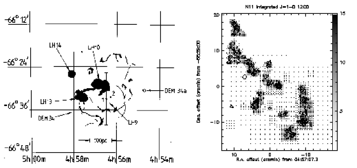
Figure 1: Left: N 11 sketch from Meaburn et al. (1989). H$\alpha$ emission is marked by dark zones; OB associations are indicated by their LH numbers (see text). Right: Overall distribution of integrated $J$=1–0 $\,{\rm{}^{12}CO}$ emission in N 11 on the same scale.

Table 1: Catalogue of CO clouds in N 11

No.	N11a	LI-LMCb	LMC-Bc	Cloud Centerd		Peak $J$=1-0 CO Parameters				Peak $J$=2-1 CO Parameters
				$\Delta\alpha$	$\Delta\delta$	Tmb	$\Delta$V	$V_{\rm LSR}$	$I_{\rm CO}$	Tmb	$\Delta$V	$V_{\rm LSR}$	$I_{\rm CO}$
				$(^{\prime})$	$(^{\prime})$	(K)	($\,{\rm{km\,s^{-1}}}$)		($\,{\rm{K\,km\,s^{-1}}}$)	(K)	($\,{\rm{km\,s^{-1}}}$)		($\,{\rm{K\,km\,s^{-1}}}$)
1		190		-10.0	-5.0	1.25	2.7	280.8	3.6$\pm$0.5
2	H	190		- 9.5	-3.7	1.57	2.7	276.3	4.5$\pm$0.6
3		192		-9.5	-8.2	1.39	2.9	284.4	4.2$\pm$0.4
4	I	192		-9.4	-10.0	2.56	5.7	279.0	15.6$\pm$2.0
5	(G)	195		-8.5	-0.5	2.21	4.0	272.9	9.4$\pm$0.9
6		205		-6.3	-13.5	2.61	2.5	277.7	6.8$\pm$1.0
7		205		-5.0	-12.5	2.04	1.9	280.8	4.2$\pm$0.6	3.27	5.0	278.4	17.5$\pm$0.5
8	F	214	0456-6636	-4.4	-7.4	2.42	2.6	276.6	6.6$\pm$0.8	2.68	3.0	276.4	8.4$\pm$0.4
9	F	214	0456-6636	-3.0	-8.0	1.46	2.6	268.6	4.0$\pm$0.6
10	B	217	0456-6629	-2.5	0	2.47	6.1	285.6	16.0$\pm$1.7	5.53	5.8	285.4	34.1$\pm$0.4
11	A	226		0.3	1.0	1.33	4.5	277.1	6.4$\pm$0.7	3.13	4.7	276.8	15.9$\pm$0.5
12	J	229		0.3	6.0	1.56	4.4	279.6	7.2$\pm$1.0
13		226		1.0	2.2	1.39	3.1	283.1	4.6$\pm$0.6	1.53	2.7	278.8	4.1$\pm$0.5
14	C	243	0457-6632	2.9	-2.3	0.96	4.0	280.2	4.4$\pm$0.9	3.32	4.0	279.6	14.3$\pm$0.4
15	D	248	0457-6632	3.7	-4.3	3.00	3.8	280.7	12.0$\pm$2.0	3.82	4.0	280.8	16.3$\pm$0.5
16	E	251	0458-6626	4.6	3.8	1.50	5.8	268.1	9.3$\pm$1.3
17	E	251	0458-6626	4.2	4.2	1.46	1.7	275.2	2.6$\pm$0.4
18	E		0458-6626	5.3	5.5	2.53	3.9	271.2	10.9$\pm$1.0	2.91	4.6	271.0	14.3$\pm$0.4
19				6.4	6.8	1.54	3.7	271.3	6.0$\pm$0.9
20				7.4	8.3	0.57	8.3	275.4	6.0$\pm$0.9
21				8.7	9.2	1.14	4.8	277.0	5.8$\pm$0.7
22				8.7	9.7	1.32	2.0	284.1	2.8$\pm$0.9
23		268		9.0	7.5	0.58	8.0	274.7	4.9$\pm$0.6
24		268		11.0	7.7	1.47	3.1	278.8	3.3$\pm$1.0
25			0458-6616	10.2	12.2	0.89	3.0	273.1	2.8$\pm$0.6
26			0458-6616	10.8	11.1	1.85	2.0	281.0	3.9$\pm$0.6
27		266		9.8	14.7	2.01	3.9	278.4	8.5$\pm$0.0
28		271		9.4	16.4	2.87	3.9	276.8	11.3$\pm$0.4	1.59	4.1	277.1	6.9$\pm$0.4
29		271		10.0	17.4	2.49	3.2	275.4	8.5$\pm$0.4	2.78	4.6	274.7	13.6$\pm$0.5

Notes: ^a Henize (1956) designation ^b IRAS source: Schwering $\&$ Israel (1990). ^c Radio continuum source: Filipovic et al. (1996). ^d Offsets refer to central mapping position (epoche 1950.0) $\alpha_{\rm o}=04^{h}57^{m}07.^{s}3$, $\delta_{\rm o}=-66^{\rm o}29^{\prime}00^{\prime\prime}$.

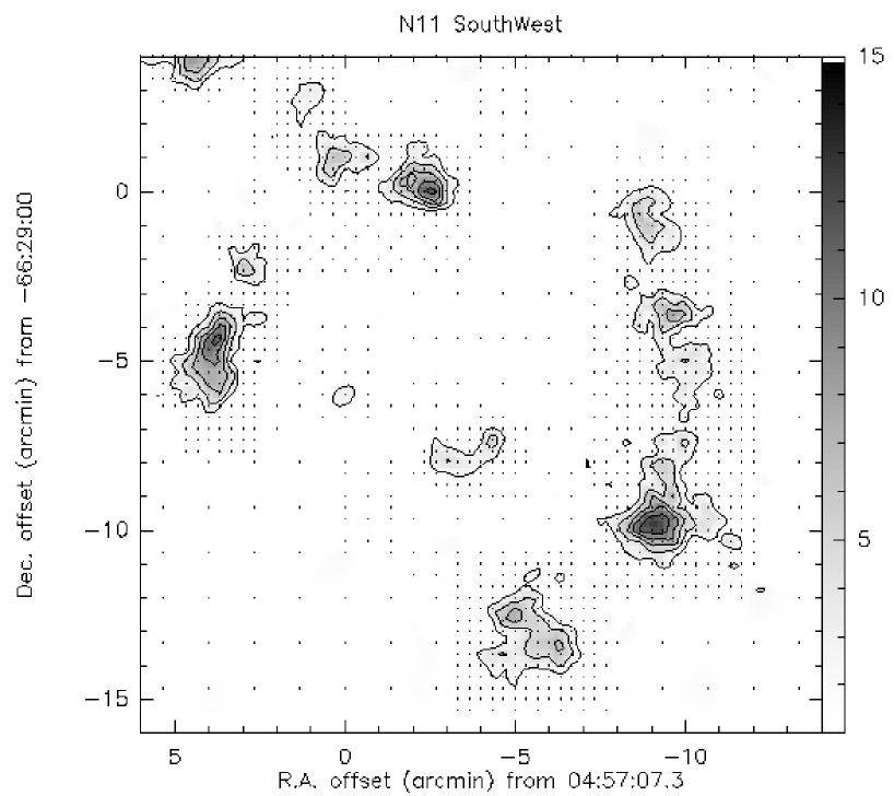
Figure 2: Detailed map of the integrated $J$=1–0 $\,{\rm{}^{12}CO}$ emission in the southwestern part of the N11 complex, showing the ‘ring’ of CO clouds associated with OB associations LH 9, LH 10 and LH 13. Positions sampled are indicated by dots. In this Figure, and in the following, grey scales indicated at the right of the panel are integrated antenna temperatures. The contours, however, are chosen such that both the first contour and the contour interval correspond to 3 $\,{\rm{K\,km\,s^{-1}}}$ in main-beam brightness temperature.

The ESO SEST Key Programme was established to investigate the molecular gas in the nearest neighbours to the Milky Way, the Magellanic Clouds. Considerations pertinent to this programme were given by Israel et al. (1993; Paper I). Following ESO’s discontinuation of the concept of Key Programmes, the observational programme was ended in 1995, although the processing of data obtained has continued. In this paper we present the results of observations of the HII region complex N 11 (Henize 1956), located in the northwestern corner of the Large Magellanic Cloud (LMC). After 30 Doradus with its retinue of HII regions, supernova remnants and dark clouds, this complex is the second-brightest in the LMC. CO observations of the former, also made within the context of the Key Programme, have been published by Johansson et al. (1998) and Kutner et al. (1997).

The N 11 complex is also known as DEM 34 (Davies et al. 1976), and has an overall diameter of about 45^′ , corresponding to a linear extent of 705 pc for an assumed LMC distance of 54 kpc (Westerlund, 1990, but see Walker 1999). In Fig.1 we present a sketch map of the optical nebulosity. In the west, N 11 contains the small supernova remnant N 11L (= DEM 34a). From the main body of the N 11 complex, a loop of HII regions and more diffuse H$\alpha$ emission extends to the northeast. This loop delineates the eastern half of LMC supergiant shell SGS-1 (Meaburn 1980) which has a diameter of about a kiloparsec and is centered on OB association LH 15 (Lucke $\&$ Hodge 1970 – not marked in Fig. 1).

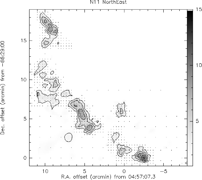
Figure 3: Detailed map of the integrated $J$=1–0 $\,{\rm{}^{12}CO}$ emission in the northeastern part of the N11 complex, showing the ‘chain’ of CO clouds associated with OB association LH 14 and supergiant shell SGS 1; otherwise as Fig. 2.

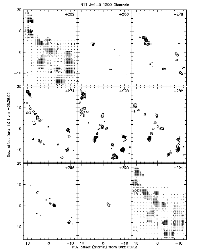
Figure 4: N11 $J$=1-0 $\,{\rm{}^{12}CO}$ channel maps. Number in top right corner indicates central velocity $V_{\rm LSR}$. Positions sampled are indicated in the maps centered on +262 and +294 $\,{\rm{km\,s^{-1}}}$. CO emission is integrated in bins of 4 $\,{\rm{km\,s^{-1}}}$ width. First contour and contour interval correspond to $\int T_{\rm mb}{\rm d}V=0.7\,{\rm{K\,km\,s^{-1}}}$.

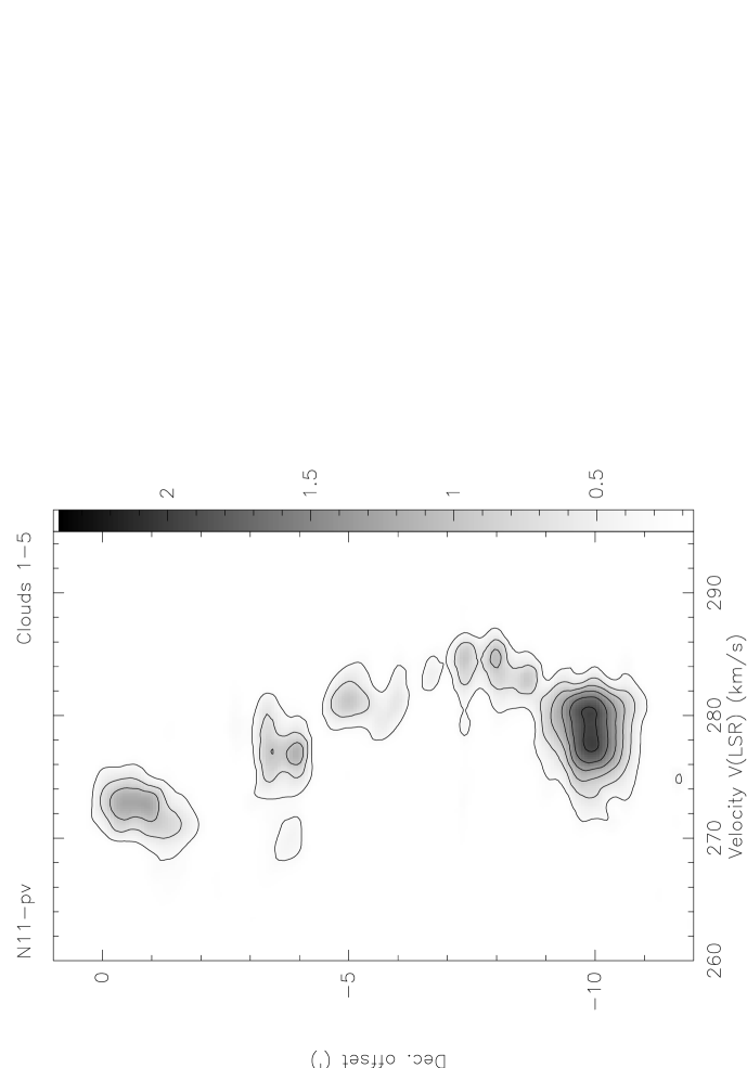
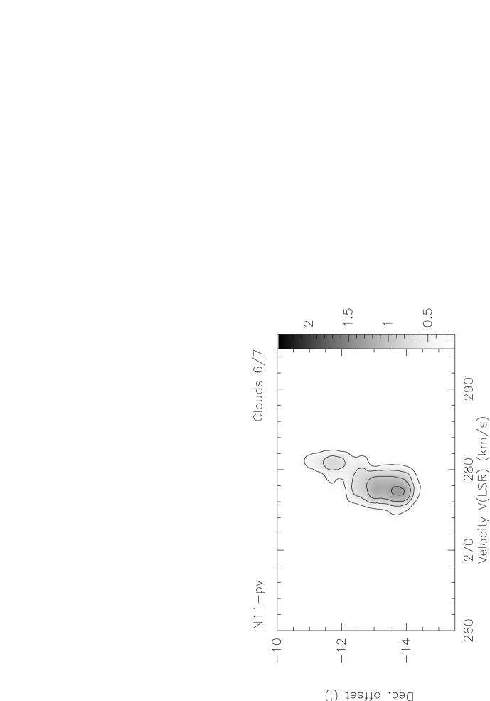
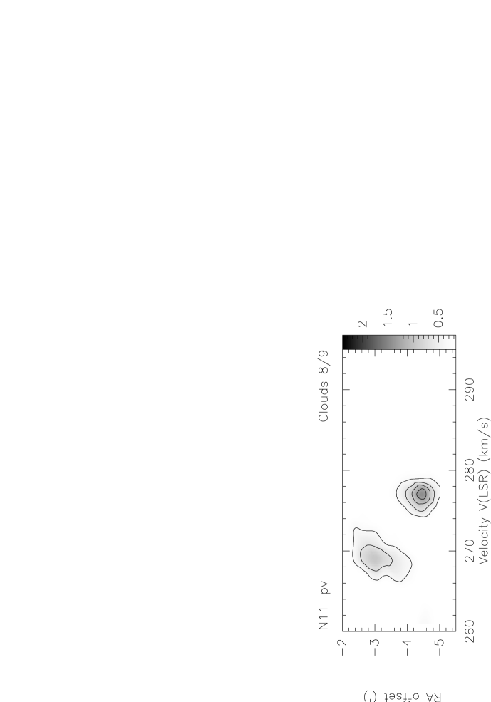
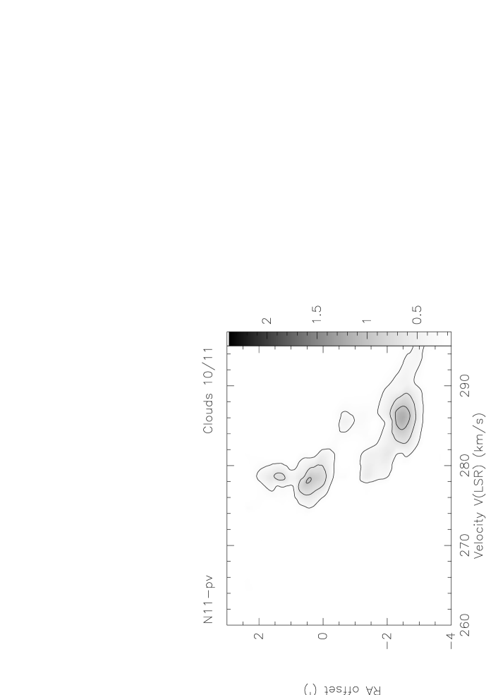
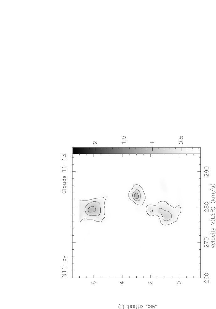
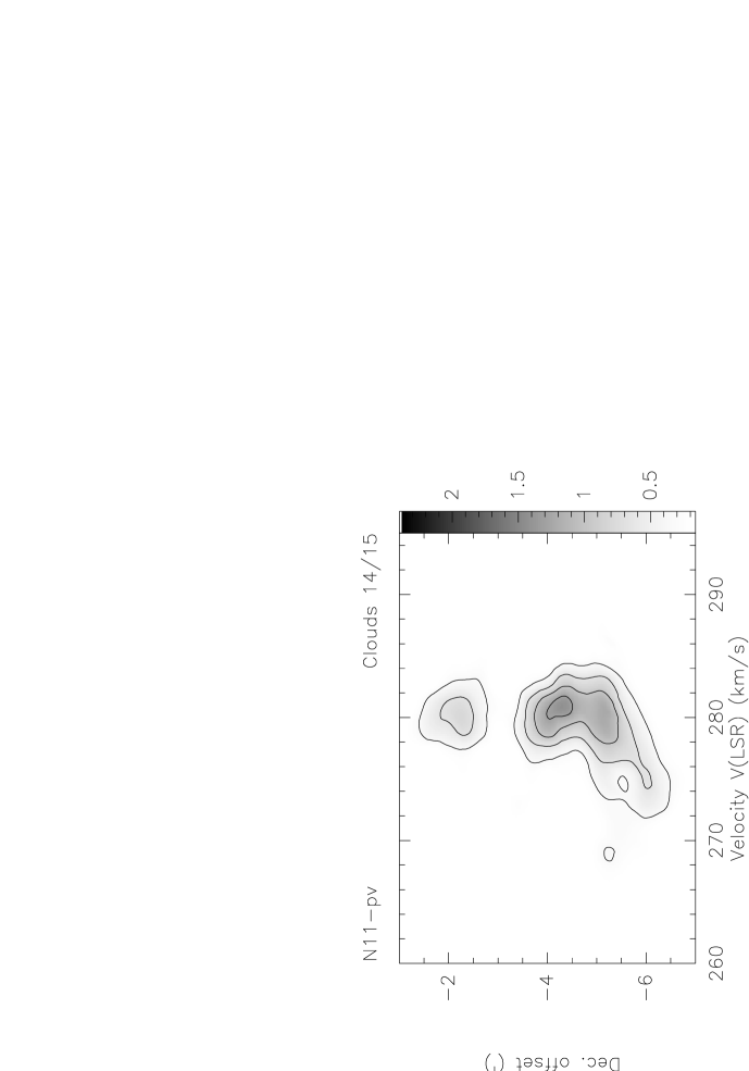
Figure 5: $J$=1-0 $\,{\rm{}^{12}CO}$ position-velocity maps for clouds 1 through 15 associated with the ‘ring’ in N 11. All maps are at constant right ascension, except those of clouds 8, 9, 10 and 11 which are at constant declination. Contours are multiples of $\int T_{\rm mb}{\rm d}V=0.46\,{\rm{K\,km\,s^{-1}}}$. Grey scales are labeled in $\int T_{\rm A}^{*}{\rm d}V$.

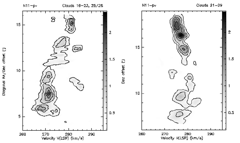
Figure 5: continued; $J$=1-0 $\,{\rm{}^{12}CO}$ position-velocity maps for clouds 16 through 29 associated with the northeastern ‘chain’ in N 11. The map for clouds 16-23 is along a diagonal originating at the map (0,0) position and extending to the northeast in position angle 45^∘ (counterclockwise). The map for clouds 21-29 is at constant right ascension. Contours are at multiples of $\int T_{\rm mb}{\rm d}V=0.46\,{\rm{K\,km\,s^{-1}}}$. Grey scales are labeled in $\int T_{\rm A}^{*}{\rm d}V$.

Table 2: Line ratios of N 11 CO clouds

No.	$\textstyle{J=2-1\over J=1-0}$	$\textstyle{\,{\rm{}^{12}CO}\over\,{\rm{}^{13}CO}}$	$\textstyle{\,{\rm{}^{12}CO}\over\,{\rm{}^{13}CO}}$
	$\,{\rm{}^{12}CO}$	$J$=1–0	$J$=2–1
4	0.7$\pm$0.2	9.4$\pm$1.4
5		14.2$\pm$2.1
7		5.1$\pm$1.1
8	1.2$\pm$0.3	7.4$\pm$1.1
10	1.2$\pm$0.3a	9.8$\pm$1.2	4.8$\pm$0.9
11	0.9$\pm$0.2a	5.3$\pm$0.8
12		7.9$\pm$1.1
13	0.7$\pm$0.3a	8.8$\pm$2.8
14	1.3$\pm$0.4a	6.0$\pm$0.8	4.7$\pm$0.9
15	1.2$\pm$0.2a	7.6$\pm$1.1
18	1.1$\pm$0.2	22.8$\pm$3.7
27		15.7$\pm$2.0
28		10.1$\pm$1.2
29		8.4$\pm$1.1

Notes: ^a average over cloud

Table 3: Properties of CO clouds in N 11

No	Luminosity	Mean	Virial	$X$
	$L_{\rm CO}$	Radius	Mass	1020 cm2
	$\,{\rm{K\,km\,s^{-1}}}$ pc2	$R$ pc	104 M⊙	$(\,{\rm{K\,km\,s^{-1}}})^{-1}$
1	2705	10.6	1.6	3.8
2	2650	7.3	1.1	2.6
3	2725	11.3	2.0	4.6
4	10470	11.2	7.6	4.6
5	3955	8.9	2.0	3.2
6	5790	19.9	2.6	2.9
7	3400	$<$5	$<$0.4	$<$0.7
8	1335	$<$5	$<$0.7	$<$3.4
9	1485	7.0	1.0	4.2
10	5720	7.4	5.4	5.9
11	2995	7.7	3.3	6.9
12	2560	7.4	3.0	7.4
13	2245	$<$5	$<$1.0	$<$2.9
14	1565	$<$5	$<$1.7	$<$6.8
15	9290	10.7	3.2	2.2
16	2890	7.7	5.4	11.8
17	1400	8.6	0.5	2.4
18	4385	8.5	2.7	3.9
19	2725	9.0	2.6	5.9
20	1190	$<$5	$<$7.2	$<$38
21	1885	6.9	3.3	11.2
22	850	6.0	0.5	3.7
23	3505	—	—	—
24	1660	8.3	1.7	6.3
25	510	$<$5	$<$1.0	$<$12
26	1925	10.4	0.9	2.8
27	1970	6.1	1.6	5.0
28	3915	7.4	2.0	3.2
29	2615	$<$5	$<$1.1	$<$2.6

N 11 is prominent not only at optical wavelengths, but also in the infrared and radio continua (Schwering $\&$ Israel 1990; Haynes et al. 1991) and in CO line emission (Cohen et al. 1988). It has a complex structure (see Fig. 1). The southern part of N11 appears to be a filamentary shell of diameter 200 pc enclosing the OB association LH 9 (Lucke $\&$ Hodge 1970) also known as NGC 1760. In the center of this shell, we find the relatively inconspicuous HII-region N 11F. At the northern rim of the shell, another OB association, LH 10 (a.k.a. NGC 1763, IC 2115, IC 2116) is associated with the very bright HII region N 11B and the bright, compact object N 11A (Heydari-Malayeri $\&$ Testor 1983). The eastern rim of the shell is likewise marked by the OB association LH 13 (NGC 1769) exciting the bright HII regions N 11C and N 11D. Finally, OB association LH 14 (NGC 1773), coincident with HII region N 11E, marks the point where the northeastern loop SGS-1 meets the filamentary shell around LH 9. The HII regions N 11B, N 11CD, N 11E and N 11F are all identified with thermal radio sources in the catalog published by Filipovic et al. (1996). The far-infrared emission from warm dust does not show the same spatial distribution as the radio continuum and H$\alpha$ line emission from ionized hydrogen gas (see Fig. 3 in Xu et al. 1992). The latter fills the whole shell region, whereas the former is clearly enhanced at the shell edges. The radio HII regions have typical r.m.s. electron-densities of 15 $\,{\rm cm^{-3}}$, masses of $10^{4}-10^{5}$ M_⊙, emission measures of $10^{4}$ pc cm^-6 and appear to be well-evolved (Israel 1980). The OB associations powering the complex are all rich associations. For instance, LH 9 contains 28 O stars, and LH 10 contains 24 O stars (Parker et al. 1992). Likewise, LH 13 contains some 20 O stars, and LH 14 about a dozen (Heydari-Malayeri et al. 1987). It is possble that star formation in the N 11 complex is at least partly triggered by the expanding shell surrounding LH 9 (Rosado et al. 1996).

The low-resolution (12^′) CO observations by Cohen et al. (1988) showed that the N 11 group of HII regions is associated with an extended molecular cloud complex. It is the third brightest CO source in their survey, after the very extended 30 Doradus complex, and the more modest N 44 complex. Cohen et al. estimated for the N 11 molecular complex a mass of about $M(\,{\rm H_{2}})=5\times 10^{6}$ M_⊙, although the comparison of these data with IRAS results by Israel (1997) suggests about half this value. A higher-resolution (2.6^′) CO survey, carried out by Mizuno et al. (2001) had insufficient sensitivity to reproduce the actual CO structure; the low (virial) mass estimate given appears to be rather uncertain. Using the same instrument, Yamaguchi et al. (2001) conducted a more sensitive survey in which extended emission from a CO cloud complex is seen to follow the outline of the ionized gas making up the HII region complex.

Because of its prominence and its interesting optical structure, we have mapped N 11 and its surroundings in the $J$=1–0 $\,{\rm{}^{12}CO}$ transition within the framework of the ESO-SEST Key Programme. Preliminary results have been presented by Israel $\&$ de Graauw (1991) and Caldwell $\&$ Kutner (1996). We have also mapped parts of the complex in the $J$=2–1 $\,{\rm{}^{12}CO}$ transition, and in the corresponding transitions of $\,{\rm{}^{13}CO}$.

2 Observations

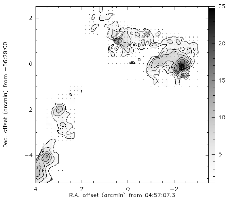
Figure 6: Velocity-integrated $J$=2-1 $\,{\rm{}^{12}CO}$ map of the northeastern segment of the ring, containing clouds 10, 11, 13, 14 and 15. Contours are at multiples of $\int T_{\rm mb}{\rm d}V=4\,{\rm{K\,km\,s^{-1}}}$. Grey scales are labeled in $\int T_{\rm A}^{*}{\rm d}V$.

The $\,{\rm{}^{12}CO}$ (1–0) observations were mostly made in a single observing run in December 1988 and January 1989 using the SEST 15 m located on La Silla (Chile). Smaller data sets obtained in April 1988 and in October 1989 were also used. The $\,{\rm{}^{12}CO}$ (2-1) measurements were made during four runs in 1989, 1992, 1993 and 1994. Although some $\,{\rm{}^{13}CO}$ $J$=1–0 observations had already been made in 1988, most were obtained during the 1993 and 1994 runs; the relatively few $\,{\rm{}^{13}CO}$ $J$=2–1 observation were all made in the 1992 run. All $J$=1–0 observations were made with a Schottky receiver, yielding typical overall system temperatures $T_{\rm sys}$ = 600 – 750 K. The $J$=2–1 observations were made with an SIS mixer, yielding typical overall system temperatures $T_{\rm sys}$ = 450 – 750 K depending on weather conditions. On average, we obtained 1$\sigma$ noise figures in a 1 km s^-1 band of 0.04, 0.10, 0.08 and 0.12 K at 110, 115, 220 and 230 GHz respectively.

In both frequency ranges, we used the high resolution acousto-optical spectrometers with a channel separation of 43 kHz. The $J$=1–0 observations were made in frequency-switching mode, initially (1988) with a throw of 25 MHz, but subsequently with a throw of 15 MHz. The $J$=2–1 measurements were made in double beam-switching mode, with a throw of 12^′ to positions verified from the $J$=1–0 $\,{\rm{}^{12}CO}$ map to be free of emission. Antenna pointing was checked frequently on the SiO maser star R Dor, about 20^∘ from the LMC; r.m.s. pointing was about $3^{\prime\prime}-4^{\prime\prime}$. The N 11 area was first roughly sampled in the $J$=1–0 $\,{\rm{}^{12}CO}$ transition on a grid of $80^{\prime\prime}$ (double-beam) spacings, using IRAS infrared maps (Schwering $\&$ Israel 1990) as a guide. Where emission was detected, we refined the grids to a half-beam sampling of $20^{\prime\prime}$. Some of the clouds thus mapped in $J$=1–0 $\,{\rm{}^{12}CO}$ were observed in $J$=1–0 $\,{\rm{}^{13}CO}$ on the same grid, and with $10^{\prime\prime}$ grid-spacing in the $J$=2–1 transitions.

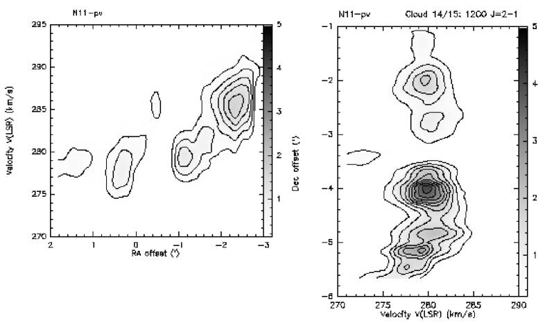
Figure 7: Position-velocity maps through clouds depicted in Fig. 6. Left: right-ascension cut at constant declination through clouds 10 and 11, with contours at multiples of $\int T_{\rm mb}{\rm d}V=0.5\,{\rm{K\,km\,s^{-1}}}$. Emission was averaged over 1 arcmin in declination. Velocity resolution $1\,{\rm{km\,s^{-1}}}$. Right: declination cut at constant right ascension through clouds 14 and 15, with contours at multiples of $\int T_{\rm mb}{\rm d}V=0.75\,{\rm{K\,km\,s^{-1}}}$. Emission was averaged over 1 arcmin in right ascension. Velocity resolution $2\,{\rm{km\,s^{-1}}}$. In both panels, grey scales are labeled in $\int T_{\rm A}^{*}{\rm d}V$.

Unfortunately, frequency-switched spectra suffer from significant baseline curvature. For N11 we corrected baselines by fitting polynomials to the baselines, excluding the range of velocities covered by emission and the ranges influenced by negative reference features. The emission velocity range was determined by summing all observations. Inspection by eye suggested that this method worked well. It has the advantage that, in principle, it does not select against weak extended emission, as long as this covers the same velocity range as the brighter clouds.

The FWHM beams of the SEST are $45^{\prime\prime}$ and $23^{\prime\prime}$ respectively at frequencies of 115 GHz and 230 GHz. Nominal main-beam efficiencies $\eta_{\rm mb}$ at these frequencies were 0.72 and 0.57 respectively. For a somewhat more detailed discussion of the various efficiencies involved, we refer to Johansson et al. (1998; Paper VII).

3 Results and analysis

3.1 Catalogue of CO clouds

An overview of the $J$=1–0 $\,{\rm{}^{12}CO}$ mapping results is shown in Fig. 1, directly comparable to the sketch of optical emission. More detailed maps of the southwestern and northeastern parts of the N 11 complex are shown in Figs. 2 and  3 respectively. Kinematical information is represented by channel maps in Fig. 4 and position-velocity maps along selected cuts in Fig. 5. The distribution of CO emission in the N 11 complex is remarkable. Using both position and kinematical information, at least 29 well-defined individual clouds can be identified. The actual number of clouds is higher than this. For instance, the velocity widths of clouds 4, 16, 20, 23, and perhaps cloud 10 as well, suggest that clouds with different velocities, but in the same line of sight, are blended together. Moreover, in the sparsely sampled parts of the map, clouds with relatively weak emission may have escaped our attention. For instance, inspection of individual profiles reveals that weak, but significant emission (typically $T_{\rm mb}\approx 0.3$ K, $\int{T_{\rm mb}{\rm d}V\approx 2\,{\rm{K\,km\,s^{-1}}}}$) is present at some positions in the map. This is the case just outside the southwestern edge of the ‘ring’ at positions (-10.7, -14.7) and (-13.3, -12), velocity $V_{\rm LSR}=274\,{\rm{km\,s^{-1}}}$, outside the southeastern edge at position (4, -14.7), velocity $V_{\rm LSR}=277\,{\rm{km\,s^{-1}}}$ and inside the ‘ring’ at (0, -6) with $V_{\rm LSR}\approx 276\,{\rm{km\,s^{-1}}}$. In the ‘empty’ southeastern part of the ring, very weak emission is likewise found at velocities between 274 and 284 $\,{\rm{km\,s^{-1}}}$, whereas stronger emission ($T_{\rm mb}\approx 0.4$ K) occurs in the gap between clouds 5 and 10, at velocities of 267 and 280 $\,{\rm{km\,s^{-1}}}$. Finally, extended weak emission appears to be present around (-7, -9) with $V_{\rm LSR}=272\,{\rm{km\,s^{-1}}}$.

All well-defined clouds and their observational properties, are listed in Table 1 which also identifies the corresponding IRAS infrared source and radio continuum sources from the catalogues by Schwering $\&$ Israel (1990) and Filipovic et al. (1996). For each cloud, we give the central position and the parameters of the peak antenna temperature $J$=1–0 and $J$=2–1 $\,{\rm{}^{12}CO}$ profiles. Clouds can readily be identified by referring the position in Table 1 to Fig. 1.

3.2 Lack of diffuse emission

The appearance of N 11 is rather different from that presented by cloud complexes in quiescent, non-star-forming regions of the LMC, such as the cloud complexes discussed in Paper VI (Kutner et al. 1997): compare in particular our Fig. 4 with their Fig. 4. In the latter, long chains of individual bright clouds are connected by continuous, relatively bright intercloud emission. The N 11 map is dominated by discrete clouds. More extended, diffuse intercloud emission is almost wholly absent, as already noted by Caldwell $\&$ Kutner (1996). By summing emission from many ‘empty’ positions, we have found that there is no diffuse emission above $T_{\rm mb}\approx 0.07$ K anywhere in the southwestern part of the N 11 complex (Fig. 2), so that the clouds in the ‘ring’ region thus have a very high contrast with their surroundings. Some amount of diffuse emission is present in the chain of clouds extending to the northeast (cf. Fig. 3). We may quantify the lack of diffuse emission by comparing the sum of the individual cloud CO luminosities in Table 1 ($\Sigma{L_{\rm CO}=9.0\times 10^{4}\,{\rm{K\,km\,s^{-1}}}{\rm pc}^{2}}$) to the independently determined integral CO luminosity from the whole N 11 map ($\int{L_{\rm CO}=11.0\times 10^{4}\,{\rm{K\,km\,s^{-1}}}{\rm pc}^{2}}$). It thus appears that, overall, the identified discrete CO clouds alone provide already 82$\%$ of the total CO emission. As may be surmised from the above, the fractions are different for the southwestern ring region and the northeastern chain. For these map areas, we find values of 93$\%$ and 75$\%$ respectively. This means that, in an absolute sense, the northeastern chain contains twice as much diffuse CO as the ring region.

3.3 Individual cloud properties

Although 22 out of 29 of the clouds listed in Table 1 are resolved, virtually all of them have dimensions no more than a few times the size of the $J$=1–0 $\,{\rm{}^{12}CO}$ observing beam. The maps in Figs. 1 through  5 therefore do not provide much information on the actual structure of individual clouds. In order to determine cloud CO luminosities and mean radii, we made for each cloud a small map (not shown) over the relevant range of positions and velocity. Cloud CO luminosities were determined by integrating these maps. We verified that the results were not significantly affected by the precise size and velocity limits of the maps. Characteristic cloud dimensions were determined by dividing the map integral by the map peak and taking the square root. The radii thus obtained were then corrected for finite beamwidth, the beam FWHM diameter of 43^′′ corresponding to a linear diameter of 11.2 pc.

The twice higher angular resolution of the $J$=2–1 $\,{\rm{}^{12}CO}$ maps shown in Fig. 6 and  7 does provide some structural information at least for clouds 10, 11, 13, 14 and 15 in the relatively bright northeastern segment of the ring. In all cases, the cloud structure thus revealed is one of mostly low-brightness CO emission with the confinements of the $J$=1–0 source extent in which a few essentially unresolved components are embedded. The overall extent of these compact components is thus significantly less than 5 pc.

Figure 8: The various parameters of the N 11 cloud ensemble do not appear to define very clear relationships. Left: Cloud velocity width d$V$ as a function of deconvolved radius $R$. Center: CO luminosity $L_{\rm CO}$ as a function of deconvolved radius $R$. Right: Virial mass $M_{\rm vir}$ as a function of CO luminosity $L_{\rm CO}$. Filled hexagons represent actual values, open hexagons represent upper limits to cloud size (left panel) or to cloud virial mass (right panel).

Although it is by no means certain that the clouds identified by us are indeed virialized, we have used the data given in Tables 1 and 3 to calculate virial masses following:

$M_{\rm vir}/{\rm M_{\odot}}={\rm k}\,R/{\rm pc}\,(\Delta V/{\,{\rm{km\,s^{-1}}}})^{2}$

where k = 210 for homogeneous spherical clouds and k = 190 for clouds with density distributions $\propto r^{-1}$ (MacLaren et al. 1988). In our calculations, we have assumed the former case, although the actual uncertainties are in any case much larger than the difference between the two values of k. The results are included in Table 3.

In previous papers we have found that cloud size, linewidth, luminosity and virial mass appear to be related quantities, although the precise form of the relations is different for SMC (Rubio et al. 1993) and LMC (Garay et al. 2002). Using data from Tables 1 and 3, we have investigated these relations also for the clouds in the N 11 complex. Fig. 8 we present the results, including the formal least-squares fits :

log d$V$ = 1.01 log $R$ – 0.39,

log $L_{\rm CO}$ = 0.94 log d$V$ + 2.96

log $M_{\rm vir}$ = 0.88 log $L_{\rm CO}$ + 1.27

Compared to the clouds studied before, those in N 11 complex are characterized by a relatively limited span in all parameters. The velocity width and linear size in particular cover only a very limited range. In addition, the diagrams in Fig. 8 exhibit a relatively large and mostly intrinsic scatter of data points. Not surprisingly, therefore, are the very small determination coefficients $r^{2}\approx 0.1$ of the d$V-R$ (left panel) and $L_{\rm CO}-$d$V$ (center panel) relations. Thus, unlike the clouds studied before in both the LMC and the SMC, the N 11 clouds do not appear to exhibit a significant correlation between these quantities.

However, the relation between cloud virial mass and and CO luminosity (right panel) seems better defined, with a determination coefficient $r^{2}\approx 0.6$. We note that the regression fit, shown in Fig. 8, has a slope very similar to the one found by Garay et al. (2002) for clouds in 30 Doradus and the surrounding LMC environment (and rather different from the one obtained for SMC clouds by Rubio et al. 1993). At the same time, for identical CO luminosities cloud virial masses are systematically $\it lower$ in the N 11 complex than in the Doradus clouds by a factor of 2.5. Leaving aside any speculation as to the origin of these differences, we feel confident to conclude that the N 11 cloud properties differ significantly from those studied at other locations either within the LMC or the SMC.

3.4 CO cloud physical condition

We have determined $J$=1–0 $\,{\rm{}^{12}CO}/\,{\rm{}^{13}CO}$ line ratios for half the clouds listed in Table 1. These ratios were usually measured near but not precisely at the integrated $\,{\rm{}^{12}CO}$ peaks. Moreover, in most cases the ratio was measured at various positions. The intensity-weighted means of these measurements and their errors are listed in Table 2. Individual values for this ratio (which we will call the isotopical ratio) range from 5 to 23, with a mean of about 10 (Table 2). Two similar determinations in the $J$=2–1 transition yield a value of about 5.

For five clouds we could integrate the $\,{\rm{}^{12}CO}$ emission in the $J$=1–0 and $J$=2–1 transitions over identical areas, thus obtaining the $J$=2–1/$J$=1–0 line ratio (i.e the transitional ratio) listed in Table 2 as ‘average over cloud’. for another three clouds we mapped small crosses in the $J$=2–1 transition, allowing us to extrapolate to the larger $J$=1–0 beam size. The transitional ratios thus derived are typically 1.2. However, the bright clouds 4 and 13 are exceptional in having the much lower value of only 0.7.

We have run radiative transfer models as described by Jansen (1995) and Jansen et al. (1994) in an attempt to reproduce the observed ratios as a function of input parameters such as molecular gas kinetic temperature $T_{\rm k}$, molecular hydrogen gas density $n_{\,{\rm H_{2}}}$ and CO column density per unit velocity $N(CO)$/d$V$. Although the models assume a homogeneous, plane-parallel geometry, this is an acceptable approximation .

Because three model parameters are required, the solutions are poorly constrained, except in the cases of clouds 10 and 14, where three line intensity ratios are available for fitting. We find that cloud 10 is best fit by a moderately dense ($n_{\,{\rm H_{2}}}=3000\,{\rm cm^{-3}}$), hot ($T_{\rm k}$ = 150 K) molecular cloud with a CO column density $N(CO)$/d$V$ = $6\times 10^{17}\,{\rm cm^{-2}}(\,{\rm{km\,s^{-1}}})^{-1}$ and a surface filling factor of 0.04 (see also, for instance, Rubio et al. 2000). In contrast, the overall beam surface filling factor is about 0.25. Although the model transitional ratio is 0.85 instead of the observed value 1.2$\pm$0.2, the model isotopical ratios are practically identical to those observed. Only one other model solution comes close to the observed value. It provides a poorer fit and requires very high densities ($n_{\,{\rm H_{2}}}=100000\,{\rm cm^{-3}}$) and very low column densities $N(CO)$/d$V$ = $0.3\times 10^{17}\,{\rm cm^{-2}}(\,{\rm{km\,s^{-1}}})^{-1}$ at low temperatures ($T_{\rm k}$ = 10 K). As Cloud 10 is very closely associated with the rich and young OB association LH 10 and the bright HII region N 11B, we consider the parameters of the first solution to be more likely correct.

However, it is unlikely that all of cloud 10 is both hot and dense. Whether or not the cloud is virialized, we expect its mass not to be very different from the value $M=5\times 10^{4}$ M_⊙ given in Table 3. To heat all of that mass to a temperature of 150 K is beyond the capacity of the OB association, even if a large fraction of it is embedded and not yet properly identified. Rather, we suspect that cloud 10 is characterized by a range of temperatures and densities, with $\,{\rm{}^{12}CO}$ emission preferentially dominated by the presumably relatively small amounts of hot gas, while the $\,{\rm{}^{13}CO}$ intensities are more susceptible to more widespread denser gas. Although the present observations do not allow fitting of such a multi-component model, future observations of higher $\,{\rm{}^{12}CO}$ and $\,{\rm{}^{13}CO}$ transitions will make this easily possible.

Clouds 14 and 15 are less closely associated with the OB association LH 13 and the HII regions N 11C/N 11D. The model solution that provides the best fit requires again moderate densities ($n_{\,{\rm H_{2}}}=3000\,{\rm cm^{-3}}$) and moderate temperatures ($T_{\rm k}$ = 60 K), together with a slightly lower column density $N(CO)$/d$V$ = $3\times 10^{17}\,{\rm cm^{-2}}(\,{\rm{km\,s^{-1}}})^{-1}$ and a surface filling factor of about 0.08. The overall beam surface filling factor is of the order of 0.3. Other solutions found, yielding higher temperatures at lower densities, and vice versa, again provide poorer fits. The temperature and mass constraints for Clouds 14 and 15 are not as stringent as those for Cloud 10, but the same comment should also apply to them.

Finally, although the lack of information does not properly constrain possible solutions, the rather high $J$=1–0 isotopical ratio of 23 for Cloud 18 does suggest a combination of relatively high densities and temperatures.

3.5 Molecular gas mass

There are various ways in which to estimate the total molecular ($\,{\rm H_{2}}$) mass from CO observations. Unfortunately, it is doubtful which of these, if any, is applicable to N 11. The presence of so many early-type stars in the immediate vicinity of the molecular material leads one to suspect that the resulting strong radiation fields have led to considerable processing of the molecular interstellar medium in N 11. The observations appear to bear this out: the lack of diffuse CO, as well as the large and apparently intrinsic scatter in the log d$V$–log$R$ and log$L_{\rm CO}$–log d$V$ diagrams (Fig. 8), the various manner in which the detected CO clouds are associated with FIR dust emission (cf. Table 1) and the elevated temperatures found above all suggest that in this complex CO has been subject to different but considerable degrees of photo-processing and photo-dissociation.

The kinematics of the clouds do not suggest regular rotation, or any other systematic movement, precluding a dynamical mass determination. For the same reason, it is very difficult to relate the present results to the overall structures such as shells etc that may have resulted from the interaction of the many OB stars in the region with the ambient interstellar medium. Obviously, the virial theorem cannot be applied to the cloud ensemble defining the ring, nor to that forming the northeastern ridge of clouds. The way in which the barely resolved $J$=1–0 clouds break up in equally barely resolved $J$=2–1 clouds also casts some doubt on the applicability of the virial theorem to the individual clouds, and Fig. 8 does not show a very tight relation between virial mass and CO luminosity. Finally, there is now ample evidence that the ‘standard’ CO-to-$\,{\rm H_{2}}$ conversion factor $X$ that is often used to derive molecular hydrogen column densities from CO luminosities is not valid under the very circumstances pertaining to N 11: strong radiation fields and low metallicities (Cohen et al. 1988; Israel, 1997; see also discussion in Johansson et al. 1998).

Comparison of the virial masses, corrected for a helium contribution of 30$\%$ by mass, with the observed CO luminosity supplies the mean CO-to-$\,{\rm H_{2}}$ conversion factor $X$, following:

$X=1.0\times 10^{22}\,R\,(\Delta V^{2})\,L_{\rm CO}^{-1}$

The values $X$ thus calculated are also listed in Table 3. We find for the discrete CO clouds a range of $X$ values between $2\times 10^{20}$ and $12\times 10^{20}\,{\rm cm^{-2}}(\,{\rm{K\,km\,s^{-1}}})^{-1}$, with a mean $X$ = $5\pm 0.5\times 10^{20}\,{\rm cm^{-2}}(\,{\rm{K\,km\,s^{-1}}})^{-1}$, i.e. 2.5 times the ‘standard’ conversion factor in the Solar Neighbourhood. Johansson et al. (1998) and Garay et al. (2002) obtained similar results for clouds in the 30 Doradus region and Complex 37 respectively.

These factors can also be compared to those determined independently for the whole complex by Israel (1997, hereafter I97). From a comparison of observed far-infrared, HI and CO intensities, i.e. explicitly taking all HI in the nebular complex into account, he finds $X$(N 11-ring) = $21\pm 9\times 10^{20}\,{\rm cm^{-2}}(\,{\rm{K\,km\,s^{-1}}})^{-1}$ and $X$(N11-northeast) = $6\pm 2\times 10^{20}\,{\rm cm^{-2}}(\,{\rm{K\,km\,s^{-1}}})^{-1}$. As discussed by Israel (2000), the conversion factor for whole complexes is expected to be higher than that of the individual constituent CO clouds. In the latter case, spatial volumes that contain abundant and selfshielding $\,{\rm H_{2}}$ but have little or no CO left, are explicitly excluded in the virial calculation. the result is thus biased to the volumes least affected by photo-processing. Measurements of the whole complex avoid such a bias.

The overall conversion factor for the northeast ridge is only 25$\%$ higher than the mean for the individual clouds, hardly a significant difference. Such a value, only a few times higher than the conversion factor in the Solar Neighbourhood, is characteristic for quiescent areas in the moderately low-metallicity LMC (cf. I97), and suggests that relatively little processing has taken place in the ridge area. The sum of the observed individual cloud masses in the ridge is $M_{\rm vir}(ridge)=3.1\times 10^{5}$ M_⊙. Assuming no HI to be present in these clouds but correcting for helium, we find from this a total molecular mass for the ridge clouds $M_{\,{\rm H_{2}}}(ridge)\geq 2.2\times 10^{5}$ M_⊙. Although this is, strictly speaking, a lower limit because we did not fully map the ridge area and additional clouds may have escaped attention, we note that the more extended maps by Yamaguchi et al. (2001) suggest that in fact only a very little CO emission occurs outside the area mapped by us.

The data tabulated by I97 imply a neutral hydrogen massa $M_{\rm HI}(ridge)\approx 4\times 10^{5}$ M_⊙, presumably mostly between the clouds, and a total molecular hydrogen mass $M_{\,{\rm H_{2}}}(ridge)\approx 5.5\times 10^{5}$ M_⊙. A mass $M_{\,{\rm H_{2}}}\leq 2.5\times 10^{5}$ M_⊙ is unaccounted for by individual clouds, which should represent molecular material distributed between the CO clouds mapped and not directly observed. We have already found that the total CO luminosity observed in the ridge is about a third higher than the sum of the individual clouds. Thus, diffuse intercloud CO in the ridge will have a luminosity $L_{\rm CO}\geq 1.0\times 10^{4}\,{\rm{K\,km\,s^{-1}}}$ pc², again a lower limit because of incomplete mapping.

The situation in the ring is different. The overall conversion factor (I97) is $5\pm 2$ times higher than the mean value for the individual clouds. The total CO emission is only a few per cent higher than the cloud sum, leaving no more than $L_{\rm CO}\approx 0.5\times 10^{4}\,{\rm{K\,km\,s^{-1}}}$ pc² for the intercloud CO. The $\,{\rm H_{2}}$ mass contained in the detected CO clouds is $M_{\,{\rm H_{2}}}(ring)\approx 3.2\times 10^{5}$ M_⊙, again under the assumption that there is no atomic hydrogen contribution to the virial mass. From I97 we find, however, total ring-area masses $M_{\,{\rm H_{2}}}=16.5\times 10^{5}$ M_⊙ and $M_{\rm HI}=5.7\times 10^{5}$ M_⊙. This result therefore predicts the presence molecular hydrogen not sampled by CO ($X_{intercloud}\leq 175\times 10^{20}\,{\rm cm^{-2}}(\,{\rm{K\,km\,s^{-1}}})^{-1}$) in amounts of more than twice that of atomic hydrogen. The ring is thus a rather extreme photon-dominated region (PDR), and should exhibit characteristic signposts such as strong [CI] and [CII] emission.

4 Conclusions

1. We have mapped the strong star-forming complex N 11 in the $J$=1–0 $\,{\rm{}^{12}CO}$ line. Additional data were obtained in the $J$=2–1 $\,{\rm{}^{12}CO}$ line, and in the corresponding transitions of $\,{\rm{}^{13}CO}$.

2. A total of 29 individual clouds could be identified. As the N 11 area was not completely mapped and not fully sampled, the actual number of clouds is probably higher. The clouds are distributed in a ring or shell surrounding the OB association LH 9, and in a ridge extending to the northeast which appears to be associated with the supergiant shell SGS 1.

3. With an 11 pc linear resolution, most of the clouds are barely resolved. With a twice higher resolution, most of the emission is seen to come from again barely resolved structures in these clouds. If the virial theorem is taken for guidance, the individual clouds have masses ranging from 0.5 to 7.5 $\times 10^{4}$ M_⊙, with a mean of $2.5\times 10^{4}$ M_⊙.

4. Unlike the apparently quiescent northeastern ridge, the ring region appears to be an extreme photon-dominated region (PDR). The high overall CO to $\,{\rm H_{2}}$ conversion factor $X$ of this PDR greatly contrasts with the almost ’normal’ conversion factors of individual dense CO clouds which more effectively resist the strong UV radiation from the embedded OB associations LH 9, LH 10 and LH 13.

5. There is very little diffuse CO emission between the clouds, and indeed in the N 11 complex as a whole. Nevertheless, diffuse $\,{\rm H_{2}}$ not sampled by CO because of the PDR nature of the complex should be be present in significant amounts. This is particularly true for the ring region.

- (1) Caldwell D.A., Kutner M.L. 1996 ApJ 472, 611
- (2) Cohen R.S., Dame T.M., Garay G., et al. 1988 ApJL 331, L95
- (3) Davies R.D., Elliott H.K., Meaburn J., 1976 MNRAS 81, 89
- (4) Filipovic M.D., Haynes R.F., White G.L., et al., 1996 A&AS 120, 77
- (5) Garay G., Johansson L.E.B., Nyman L.-, et al. 2002 A&A in press (Paper VIII)
- (6) Haynes R.F., Klein U., Wayte S.R., et al., 1991 A&A 252, 475
- (7) Henize H., 1956 ApJS 2, 315
- (8) Heydari-Malayeri M. Testor G., 1983 A&A 118, 116
- (9) Heydari-Malayeri M., Niemela V.S., Testor G., 1987 A&A 184, 300
- (10) Israel F.P., 1980 A&A 90, 246
- (11) Israel F.P., 1997 A&A 328, 471 (I97)
- (12) Israel F.P., 2000, in: Molecular Hydrogen in Space, eds. F. Combes G. Pineau des Forets, Cambridge Unversity Press, pp. 293-296
- (13) Israel F.P., de Graauw Th., 1991 in ‘The Magellanic Clouds’, IAU Symp. 148, Eds. R. Haynes D. Milne, Kluwer Acad. Publ.: Dordrecht, p. 45
- (14) Israel F.P. Johansson L.E.B., Lequeux J., et al. 1993 A&A 276, 25 (Paper I)
- (15) Jansen D.J., 1995, Ph.D. thesis, Leiden University (NL)
- (16) Jansen D.J., van Dishoeck E.F., Black J.H., 1994, A&A 282, 605
- (17) Johansson L.E.B., Greve A., Booth R.S., et al. 1998 A&A 331, 857 (Paper VII)
- (18) Kutner M.L., Rubio M., Booth R.S., et al. 1997 A&AS 122, 255 (Paper VI)
- (19) Lucke P.B., Hodge, P.W., 1970 AJ 75, 171
- (20) Meaburn J., Laspias V., Solomos N., Goudis C., 1989 A&A 225, 497
- (21) Meaburn J., 1980 MNRAS 192, 365
- (22) Mizuno N., Yamaguchi R., Mizuno A., et al. 2001 PASJ 53, 971
- (23) Parker J.W., Garmany C.D., Massey P., Walborn N.R., 1992 AJ 103, 1205
- (24) Rosado M., Laval A., Le Coarer, E., et al. 1996 A&A 308, 588
- (25) Rubio M., Contursi A., Lequeux J. , et al. 2000 A&A 359, 1139
- (26) Schwering P.B.W., Israel F.P., 1990, Atlas and Catalogue of Infrared Sources in the Magellanic Clouds, Kluwer, Dordrecht
- (27) Walker A.R., 1999 in: Post-Hipparcos Cosmic Candles, eds. A. Heck F. Caputo (Kluwer, Dordrecht), ApSpSc Lib. 237, p. 125
- (28) Westerlund B.E., 1990 AA R 2, 29
- (29) Xu C., Klein U., Meinert D., Wielebinski R., Haynes R.F., 1992 A&A 257, 47
- (30) Yamaguchi R., Mizuno N., Onishi T., Mizuno A., Fukui Y. 2001 PASJ 53, 959sum