Microflares in accretion disks

We have investigated the phenomenon of explosive chromospheric evaporation from an accretion disk as a mechanism for fast variability in accreting sources such as low mass X-ray binaries and active galactic nuclei. This has been done in the context of advection dominated accretion flows, allowing both high and low states to be considered. This mechanism can in principle produce sub-millisecond timescales in binaries and sub-minute timescales in active galaxies. However, even considering the possibility that large numbers of these microflares may be present simultaneously, the power emitted from these microflares probably amounts to only a small fraction of the total X-ray luminosity.

1 Introduction

All models for X-ray binaries (XRBs) involve accretion onto compact central objects. Similarly, accretion onto supermassive black holes is the dominant paradigm for the engine of active galactic nuclei (AGN). Recently, advection dominated accretion flows (ADAFs) have been advocated as a natural way of explaining the variety of states in which individual binary X-ray sources have been observed (e.g. Chakrabarti & Titarchuk chakrabarti95 (1995); Esin et al. esin97 (1997), esin98 (1998)). Rapid fluctuations have been detected in many electromagnetic bands and modeled in a wide variety of ways (e.g. Krishan & Wiita krishan94 (1994); Wagner & Witzel wagner (1995); Tanaka & Shibazaki tanaka (1996); Wiita wiita (1996)). In low-mass X-ray binaries, we are presumably dealing with accretion onto black holes (BHs) with masses typically 5–15 $M_{\odot}$, with luminosities of $L_{\rm X}\sim 10^{35-37}$ erg s^-1 in the low/hard state, and with fast variations detectable down to $0.01$ s (e.g. Esin et al. esin97 (1997), esin98 (1998); Tanaka & Shibazaki tanaka (1996); Trudolyubov et al. trudolyubov (2001)). Seyfert galaxies typically exhibit $L_{\rm X}\sim 10^{42-44}$ erg s^-1, with noticeable variations observed on timescales as short as minutes (e.g. Lawrence & Papadakis lawrence (1993); Turner et al. turner (1999)).

Many accretion models involve hot low-density coronae lying over high density, cooler accretion disks (e.g. Galeev et al. galeev (1979); White & Holt white (1982); Haardt et al. haardt (1994); Poutanen poutanen (1998)), and much of the resulting physics is not dissimilar to that in ADAF-type models. Recent three-dimensional magnetohydrodynamical simulations of accretion disks indicate that magnetic fields will be strengthened within the disk and that plasma and fields will escape from the disk into a strongly magnetized corona (Miller & Stone miller (2000)). This situation is reminiscent of the conditions prevailing in the solar atmosphere, and therefore, our understanding of solar flare related processes may well be carried over to accreting sources such as XRBs and AGN, which exhibit rapid variations in luminosity (e.g. Kuijpers kuijpers (1995); di Matteo dimatteo (1998); Krishan et al. krishan00 (2000)). In particular, the phenomenon of chromospheric evaporation caused by the nonthermal electron heating is often invoked to explain the rapid rise of the soft X-ray emission during flares and the blueshift of soft X-ray lines of Ca xix and Fe xxv (e.g. Antonucci et al. antonucci (1982)). This explosive evaporation has been studied using what is known as the exploding gasbag model (Fisher fisher (1987); Bastian et al. bastian (1998)). In this paper, we extend this model to conditions relevant to accretion flows in both LMXBs and AGNs, and make an approximate evaluation of its possible contribution to X-ray emission and variability.

2 Basic Model

Figure 1 illustrates the situation we have in mind. We consider an ADAF allowing for variations in the accretion rate, ${\dot{M}}$, and thus in the transition radius, $r_{t}$, which is thereby capable of reproducing the spectrum of X-ray binaries in both their low/hard state and high/soft states (e.g. Esin et al. esin97 (1997)). The low (high) state is presumed to correspond to low (high) values of the accretion rate, normalized to the Eddington accretion rate, ${\dot{m}}={\dot{M}}/{\dot{M}}_{\rm Edd}$. For larger values of ${\dot{m}}$ the ADAF region shrinks ($r_{t}$ decreases)(e.g. Abramowicz et al. abramowicz (1996); Narayan et al. narayan97 (1997)); specific ranges of $\dot{m}$ are capable of producing the quiescent, intermediate and very-high states observed in some BH XRBs, such as Nova Muscae 1991 (Esin et al. esin97 (1997)), Cygnus X-1, GRO J0422+32 and GRO J1719$-$24 (Esin et al. esin98 (1998)), but we shall not be concerned with those details here. The two temperature plasma within the ADAF region extends into a corona above (at least the inner portion of) the thin accretion disk. We assume that there is significant flare activity produced through magnetic reconnection within this corona (e.g. Kuijpers kuijpers (1995)). Such releases of magnetic energy are presumably concentrated near the inner boundary of the disk where the densities and field strengths within the disk are greatest (e.g. Chakrabarti & D’Silva chakrabarti94 (1994)), and thus we will consider parameters relevant to this region.

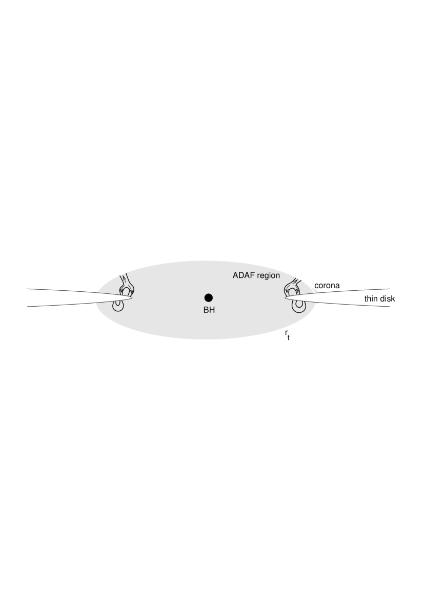
Figure 1: A schematic of an accretion flow in the low-state, where the transition radius, $r_{t}$, is far from the black hole (BH). The inner, two-temperature plasma extends out to $r_{t}$, with a thin disk and a corona present beyond that point. Flares within the corona produce electron beams, some of which impinge upon the cool disk and evaporate material from it into the corona.

Magnetic reconnection is now believed to be an essential component of the solar flare process (see Lakhina lakhina (2000) for a recent review). Bi-directional electron beams (i.e., propagating both towards and away from the Sun) are now understood to be a signature of the magnetic reconnection process as revealed through solar radio observations (e.g. Robinson & Benz robinson (2000)). Here we investigate conditions under which the “chromospheric evaporation” induced by downgoing electron beams (e.g. Fisher fisher (1987); Bastian et al. bastian (1998)) could operate in ADAF type accretion disks giving rise to rapid variability or microflares. In analogy with the solar case, we anticipate that a large number of small flares will be present simultaneously (e.g. Parker parker (1988)). The evaporation of thin disk material can erode the inner portion of the disk, thus changing $r_{t}$, and thereby possibly inducing additional X-ray variability.

3 Evaporation from accretion disks

3.1 Conditions appropriate to low states for XRBs

To illustrate this situation, we adopt simple standard $\alpha$ disk models for the outer portion of the accretion disk (e.g. Shakura & Sunyaev shakura (1973), hereafter SS), but truncate them at $r_{t}$, where the two-temperature advection dominated portion of the flow is assumed to take over. In order to incorporate the explosive gasbag (EG) model for chromospheric evaporation (e.g. Fisher fisher (1987)) we need values for the density $n_{\rm ch}$ and the scale height, $z_{0}$ in that region. At this distance from the BH, the thin disk will be characterized by gas pressure dominance over radiation pressure and electron scattering opacity larger than free-free or other opacities, so (SS),

$$h=2.3\times 10^{3}\alpha^{-1/10}m^{9/10}{\dot{m}}^{1/5}r^{21/20}{\rm cm},$$ (1)

$$n_{0}=9.2\times 10^{24}\alpha^{-7/10}m^{-7/10}{\dot{m}}^{2/5}r^{-33/20}{\rm cm}^{-3}.$$ (2)

Here, $h$ is the disk half-thickness, $\alpha$ the viscosity parameter, $m\equiv M_{\rm BH}/M_{\odot}$, ${\dot{m}}={\dot{M}}/(2.3\times 10^{-9}M_{\odot}{\rm yr}^{-1}m)$, $r=R/(2GM_{\rm BH}c^{-2})$, $n_{0}$ is the number density of the disk in the equatorial plane, and $R$ is the physical distance from the BH, so the coefficients differ from those in Shakura & Sunyaev (shakura (1973)), which uses different definitions of ${\dot{m}}$ and $r$. We have dropped the relativistic correction terms which are negligible at the distances considered here.

These standard disk models do not provide precise values for the density, $n_{\rm ch}$ and the scale height, $z_{0}$, in the photospheric/chromospheric regions of the disk. Nonetheless, an estimate for the $z_{0}$ in the photosphere, where the density falls exponentially as $n\propto{\rm exp}(-z/z_{0})$, is given by $z_{0}=r^{3}kT(z_{1})/(GMm_{p}z_{1})$, where $m_{p}$ is the proton mass and $z_{1}$ is given by the location where the total optical depth equals unity (SS). In that $z_{1}$ is only slightly greater than $z_{0}$ and the chromosphere begins at a height of at least $2z_{1}$, we adopt values of $n_{\rm ch}=1.0\times 10^{-2}\leavevmode\nobreak\ \chi\leavevmode\nobreak\ n_{0}$ and $z_{0}=0.3\leavevmode\nobreak\ \eta\leavevmode\nobreak\ h$, where we expect $\chi$, and $\eta$ to be within an order of magnitude of unity.

The microflares are likely to be concentrated in the transition region, and we use parameters relevant for low-states of ADAF models. This implies that $\dot{m}<1.3\alpha^{2}$ (e.g. Esin et al. esin97 (1997)). Most current estimates for disk viscosity involve some form of the magnetorotational instability and tend to produce $\alpha\leq 0.1$ (e.g. Brandenburg brandenburg (1998); Hawley et al. hawley (1996)), and we thus assume typical values of $\alpha_{.1}=\alpha/0.1\simeq 1$, ${\dot{m}}_{.01}={\dot{m}}/0.01\simeq 1$. For these low states, $r_{t}\sim 10^{2}-10^{4}$, so we parameterize by taking $r_{100}=r_{t}/100$. We shall first focus on LMXBs, for which a typical BH mass of $10M_{\odot}$ can be assumed, and thus use $m_{10}=M_{\rm BH}/(10M_{\odot})\simeq 1$. Then we obtain the following estimates for the scale height and density in the chromospheric regions

$$z_{0}=3.4\times 10^{5}\eta\leavevmode\nobreak\ \alpha_{.1}^{-1/10}m_{10}^{9/10}{\dot{m}}_{.01}^{1/5}r_{100}^{21/20}\leavevmode\nobreak\ {\rm cm},$$ (3)

$$n_{\rm ch}=7.3\times 10^{18}\chi\leavevmode\nobreak\ \alpha_{.1}^{-7/10}m_{10}^{-7/10}{\dot{m}}_{.01}^{2/5}r_{100}^{-33/20}\leavevmode\nobreak\ {\rm cm}^{-3}.$$ (4)

During a reconnection event, electron beams form in the current sheets; some of these will be directed downwards into the disk atmosphere and heat it. Radiative losses must be considered in this situation. In this region of the accretion disk the standard photospheric temperature is given by

$$T_{s}=1.4\times 10^{5}\alpha_{.1}^{1/75}m_{10}^{-19/75}{\dot{m}}_{.01}^{28/75}r_{100}^{-141/150}\leavevmode\nobreak\ {\rm K}.$$ (5)

The radiative loss function, $\Lambda(T)$, is maximized at temperatures near $2\times 10^{5}$K (Raymond et al. raymond (1976)), which is marginally above the value just found for $T_{s}$. Thus it is likely that such temperatures will be found in the transition region between the photosphere and the corona of the accretion disk for $r_{100}>1$, and this maximum loss rate can be achieved. In order for this evaporation mechanism to function, the minimum heating rate per particle, $Q$, must at least balance the maximum cooling rate, and is found to be $Q=\Lambda(T)n_{\rm ch}\simeq 7\times 10^{-22}{\rm erg\leavevmode\nobreak\ s}^{-1}{\rm cm}^{-3}\leavevmode\nobreak\ n_{\rm ch}$ (Fisher fisher (1987)), or

$$Q=5.1\times 10^{-3}\chi\leavevmode\nobreak\ \alpha_{.1}^{-7/10}m_{10}^{-7/10}{\dot{m}}_{.01}^{-2/5}r_{100}^{-33/20}{\rm erg\leavevmode\nobreak\ s}^{-1}.$$

If the photospheric temperature exceeds $2\times 10^{5}$K then the cooling rate drops rapidly to about $Q=1.5\times 10^{-22}n_{\rm ch}$ by $T_{s}=5\times 10^{5}$K, and then much more slowly until $T_{s}\simeq 3\times 10^{6}$K (Raymond et al. raymond (1976)). Under these cicumstances heating rates several times lower than that given above can suffice.

The energy deposited by the electron beam(s) heats the chromosphere, part of which evaporates high into the corona. If the other transport processes (e.g. conduction) are not immediately significant, then the evaporation can occur in an explosive manner and can be described by the gasbag model (e.g. Fisher fisher (1987)). Using the standard equations for mass, momentum and energy conservation, one can derive the time profiles of the plasma parameters in this gasbag. Of key importance is the timescale for build up of maximum pressure and consequent rapid evaporation of the plasma, which is found to be (Fisher fisher (1987))

$$\tau=\Bigl{(}\frac{m_{p}Z_{0}^{2}}{\pi Q}\Bigr{)}^{1/3},$$ (6)

where $m_{p}$ is the proton mass, and $Z_{0}$ is the initial thickness of the evaporating plasma. As shown by Fisher (fisher (1987)), if this EG model is to work at all, $Z_{0}$ must differ from $z_{0}$ only by a logarithmic factor not much larger than unity. For the circumstances considered here, conduction is not important until times exceeding $\sim 10\tau$, and so the time $\tau$ represents the characteristic time over which fluctuations are produced by this process. Of course, other processes which we are not considering here may well play significant roles and could produce flares by different mechanisms on different timescales. Identifying $Z_{0}=\zeta z_{0}$ with $\zeta>1$, we have the following approximate expression

$$\tau=2.3\times 10^{-4}\zeta^{2/3}\eta^{2/3}\chi^{-1/3}\alpha_{.1}^{1/6}m_{10}^{5/6}r_{100}^{5/4}\leavevmode\nobreak\ {\rm s}.$$ (7)

Therefore, for XRBs, timescales of less than a millisecond are possible for the explosive evaporation from the cool disk, even in the low state, where $r_{t}$ is at least 100.

The minimum electron flux needed for balancing the radiative losses can be approximated by

$$F\simeq Q\Bigl{(}\frac{6N_{c}}{\delta-2}\Bigr{)},$$

where $N_{c}=9.15\times 10^{18}{\rm cm}^{-2}(E_{c,10})^{2}$ (McClymont & Canfield mcclymont (1986); Fisher et al. fisheretal (1985)). Here, $\delta$ is the power-law index for the non-thermal distribution of beam electrons (in the sense that $f(E)dE\propto E^{-\delta}dE$), and the solar flare observations indicate that $\delta\simeq 4-5$ (McClymont & Canfield mcclymont (1986)). The total column density of beam electrons, $N_{c}$, is determined from collisional processes and depends upon the cut-off energy to which they can penetrate, which is typically 5–20 keV, so we use $E_{c,10}=E_{c}/10{\rm keV}\sim 1$. This electron energy flux $F$ implies densities in the beam several orders of magnitude lower than the ambient density, $n_{\rm ch}$, so the standard acceleration mechanisms invoked in solar flares are adequate (e.g. Bastian et al. bastian (1998)). Explosive evaporation occurs for fluxes greater than this minimum value, and this EG process is not relevant if the fluxes are less than this.

To obtain the total power emitted in a microflare we must estimate the area over which this flux emerges. Again, in analogy with the sun, we approximate the size, $R$, of the flaring region to be of the order of the scale height, $z_{0}$. However, it is certainly possible that the flaring loop could extend into the corona far enough so that the appropriate size is actually that of the coronal scale height, which would be several times larger (e.g. McClymont & Canfield mcclymont (1986)). Therefore, since nearly all of this power will be quickly radiated in EUV and X-ray photons, we can obtain an estimate for the minimum total power in one of these microflares as, $L_{f}=\pi R^{2}F$; taking $\delta=4$ we have,

$$L_{f}\simeq 5.1\times 10^{28}\eta^{2}\chi\alpha_{.1}^{-9/10}m_{10}^{11/10}{\dot{m}}_{0.01}^{-4/5}r_{100}^{9/20}E_{c,10}^{2}\Bigl{(}\frac{R}{z_{0}}\Bigr{)}^{2}{\rm erg\leavevmode\nobreak\ s}^{-1}.$$ (8)

The power in a single microflare $L_{f}$ is more than six orders of magnitude smaller than the total power in the low state, using our nominal values of $\eta\simeq\chi\simeq(R/z_{0})\simeq 1$, so the sobriquet microflare is quite appropriate. For these low state conditions, ($r_{t}>100$), each of these nano/micro-flares covers an area very small in comparison with the active portion of the disk ($\sim 10^{-6}$). It is essentially impossible to properly estimate the fractional area of the relevant part of the accretion disk that will be subject to this process at any particular time. However, it is certainly plausible to expect that no more than 10% of the disk should be so involved, and thus it is unlikely that $>10^{5}$ of these explosive events can be going on simultaneously. Even with this optimistic assumption, the integrated output of all these microflares is likely to remain small in comparison with the basal luminosity. Only if most of the variables in Eq. (8) exceed their nominal values could these microflares make a significant contribution to the total power. Probably the least certain factor in Eq. (8) is the ratio $R/z_{0}$, and it is not implausible that this geometrical factor could approach 10; in that case, the individual microflare luminosities rise to above $10^{-6}$ of the observed total low state power. Only in this optimistic situation is it possible that the integrated flux from all such flares could amount to a substantial fraction of the total emission. However, for large values of $R$, we expect there to be fewer of these “miniflares”, in that each now covers a larger fraction of the disk area. Hence we do not expect the integrated micro/miniflare power to rise as steeply as $(R/z_{0})^{2}$.

3.2 High/soft state conditions for XRBs

Here we consider the situation where the accretion rate is high enough so that the standard accretion flow penetrates much closer to the BH. Then the relevant equations are those appropriate for the inner portion of accretion disks, which are dominated by radiation pressure (SS). We note that for a high state, ${\dot{m}}\sim 0.1$ and $r_{t}\sim 10$ are typical parameters; furthermore, the relativistic corrections are no longer negligible, since we are dealing with regions close to the BH. With the reparameterizations ${\dot{m}}_{.1}={\dot{m}}/0.1$ and $r_{10}=r/10$, defining $B\equiv[1-(0.3/r_{10})^{1/2}]$, and still adopting $z_{0}=0.3\eta h$ and $n_{ch}=1.0\times 10^{-2}\chi n_{0}$, we find:

$$z_{0}=7.4\times 10^{4}\leavevmode\nobreak\ \eta m_{10}{\dot{m}}_{.1}B\leavevmode\nobreak\ {\rm cm},$$ (9)

$$n_{\rm ch}=4.4\times 10^{20}\chi\alpha_{.1}^{-1}m_{10}^{-1}{\dot{m}}_{.1}^{-2}r_{10}^{3/2}B^{-2}\leavevmode\nobreak\ {\rm cm}^{-3}.$$ (10)

Under these circumstances the photospheric temperature is given by

$$T_{s}=6.6\times 10^{5}\alpha_{.1}^{1/5}m_{10}^{-1/5}{\dot{m}}_{.1}^{4/5}r_{10}^{-3/2}B^{4/5}\leavevmode\nobreak\ {\rm K},$$ (11)

or $T_{s}\simeq 3.5\times 10^{5}$K for $r_{10}=1$, and all other quantities taking on their new nominal values. This somewhat exceeds the temperature at which maximum cooling occurs. It remains reasonable to utilize the value of $\Lambda$ corresponding to this higher temperature to compute the heating rate needed to compensate for cooling in the optically thin regime; for this temperature, $\Lambda$ is roughly half that of the peak.

Proceeding as in the previous subsection we then obtain,

$$Q\simeq 1.5\times 10^{-1}\leavevmode\nobreak\ \chi\alpha_{.1}^{-1}m_{10}^{-1}{\dot{m}}_{.1}^{-2}r_{10}^{3/2}B^{-2}{\rm erg\leavevmode\nobreak\ s}^{-1},$$ (12)

$$\tau=2.7\times 10^{-5}\zeta^{2/3}\eta^{2/3}\chi^{-1/3}\alpha_{.1}^{1/3}m_{10}{\dot{m}}_{.1}^{4/3}r_{10}^{-1/2}B^{4/3}\leavevmode\nobreak\ {\rm s},$$ (13)

and

$$L_{f}=7\times 10^{28}\eta^{2}\chi\alpha_{.1}^{-1}m_{10}\leavevmode\nobreak\ r_{10}^{3/2}E_{c,10}^{2}\Bigl{(}\frac{R}{z_{0}}\Bigr{)}^{2}{\rm erg\leavevmode\nobreak\ s}^{-1}.$$ (14)

In that the total power for an XRB in the high state is $\sim 10^{37}{\rm erg\leavevmode\nobreak\ s}^{-1}$, we see that each of these micro(nano?)flares contributes very little to the total power output. Of course, as for the low state, many such small scale flares may contribute simultaneously; however, in that the relevant disk area under the intense coronal region is proportional to $r^{2}$ and is thus smaller than in the low state case, the integrated contribution is very likely to be negligible.

3.3 Results for AGN

Active galactic nuclei may also be described within the ambit of ADAF models, particularly those with small output, and therefore probably low efficiency (e.g. Lasota et al. lasota (1996); Narayan et al. narayan96 (1996)) so essentially everything developed above can still be applied.

The photospheric temperatures will be significantly lower, since they decline with increasing black hole mass, but coronae and transition regions should still be present, and microflares can still evaporate disk material into the corona. Appropriate values for all dimensionless parameters are nearly the same as in the two preceding subsections. Therefore the timescales vary as $M^{5/6}$ for the low state and as $M$ for the high state. Roughly, then, these microflares operate on 3–10,000 s timescales (for $M_{BH}\sim 10^{7}-10^{8}M_{\odot})$.

Since $L_{f}\propto M^{11/10}$ for the low state and $L_{f}\propto M$ for the high state, each of these microflares could contribute between $\sim 10^{34}-10^{36}$ erg s^-1, while the total powers are $\sim 10^{40}$ erg s^-1 for low-state emission around a $10^{7}M_{\odot}$ BH up through $\sim 10^{45}$ erg s^-1 for high-state emission near a $10^{8}$ solar mass black hole. Thus, even considering the possiblity that many of these microflares can erupt simultaneously, their contribution to the total power still should be very small.

4 Conclusions

The mechanism of explosive chromospheric evaporation seems to explain some aspects of solar X-ray variability, as well as blue-shifted soft X-ray lines from the Sun. Since conditions in accretion disk atmospheres probably have many similarities to the solar case, we have explored this mechanism in the context of accretion disk models for XRBs and AGN. In particular, we have focused on the transition region in ADAF models as the most likely place for these flares and microflares to be generated. We have estimated microflare timescales and powers based on the exploding gas bag model for both low and high states for both XRBs and AGN.

We note that we have not proven that this mechanism is necessarily relevant; we have merely shown that it is plausible that it could operate in the conditions of accretion disk atmospheres, as it probably does in the Sun. Furthermore, it is very likely that other flare mechanisms dominate the observed variability. For XRBs, the EG timescales range from sub-ms to seconds, while for AGN, timescales from seconds to hours are expected, with most of the relevant emission emerging up to $\sim 10$ keV. Whereas these characteristic times are in the range of the fastest observed variability for both classes of sources, the powers in individual microflares are extremely small. However, we do expect a large number of these flares could exist essentially simultaneously, particularly in the low states. Even so, the integrated emission from these microflares is almost certainly undetectable with the current generation of X-ray telescopes.

- (1) Abramowicz, M. A., Chen, X.-M., Granath, M., & Lasota, J.-P. 1996, ApJ, 471, 762
- (2) Antonucci, E., Gabriel, A. H., Acton, L. W., et al. 1982, Sol. Phys. 78, 107
- (3) Bastian, T. S., Benz, A. O., & Gary, D. E. 1998, ARA&A, 36, 131
- (4) Brandenburg, A. 1998, Disc Turbulence and Viscosity, in Theory of Black Hole Accretion Disks, ed. M. A. Abramowicz, G. Björnsson, & J. E. Pringle (Cambridge U. Press, Cambridge), 61
- (5) Chakrabarti, S. K., & D’Silva, S. 1994, ApJ, 424, 138
- (6) Chakrabarti, S. K., & Titarchuk, L. G. 1995, ApJ, 455, 623
- (7) di Matteo, T. 1998, MNRAS, 299, L15
- (8) Esin, A. A., McClintock, J. E., & Narayan, R. 1997, ApJ, 489, 865
- (9) Esin, A. A., Narayan, R., Cui, W., Grove, J. E., & Zhang, S.-N. 1998, ApJ, 505, 854
- (10) Fisher, G. H. 1987, ApJ, 317, 502
- (11) Fisher, G. H., Canfield, R. C., & McClymont, A. N., 1985, ApJ, 289, 414
- (12) Galeev, A. A., Rosner, R., & Vaiana, G. S. 1979, ApJ, 229, 318
- (13) Haardt, F., Maraschi, L., & Ghisellini, G. 1994, ApJ, 432, L95
- (14) Hawley, J. F., Gammie, C. F., & Balbus, S. A. 1996, ApJ, 464, 690
- (15) Krishan, V., & Wiita, P. J. 1994, ApJ, 423, 172
- (16) Krishan, V., Wiita, P. J., & Ramadurai, S. 2000, A&A, 356, 373
- (17) Kuijpers, J. 1995, Flares in Accretion Disks, in Coronal Magnetic Energy Releases, ed. A. O. Benz & A. Krüger (Springer, Berlin), 135
- (18) Lakhina, G. S. 2000, Bull. Astr. Soc. India, 28, 593
- (19) Lasota, J.-P., Abramowicz, M. A., Chen, X., Krolik, J., Narayan, R., & Yi, I. 1996, ApJ, 462, 142L
- (20) Lawrence, A., & Papadakis, I. 1993, ApJ, 414, L85
- (21) McClymont, A. N., & Canfield, R. C. 1986, ApJ, 305, 936
- (22) Miller, K. A., & Stone, J. M. 2000, ApJ, 534, 398
- (23) Narayan, R., Kato, S., & Honma, F. 1997, ApJ, 476, 49
- (24) Narayan, R., Yi, I., & Mahadevan, R. 1996, A&AS, 120, 287
- (25) Parker, E.N. 1988, ApJ, 330, 474
- (26) Poutanen, J. 1998, Accretion disc-corona models and X/-ray spectra of accreting black holes, in Theory of Black Hole Accretion Disks, ed. M. A. Abramowicz, G. Björnsson, & J. E. Pringle (Cambridge U. Press, Cambridge), 100
- (27) Raymond, J. C., Cox, D. P., & Smith, B. W. 1976, ApJ, 204, 290
- (28) Robinson, P. A., & Benz, A. O. 2000, Solar Phys., 194, 345
- (29) Shakura, N. I., & Sunyaev, R. A., 1973, A&A, 24, 337 (SS)
- (30) Tanaka, Y., & Shibazaki, N. 1996, ARA&A, 34, 607
- (31) Trudolyubov, S. P., Borozdin, K. N., & Priedhorsky, W. C. 2001, MNRAS, 322, 309
- (32) Turner, T. J., George, I. M., Nandra, K., & Turcan, D. 1999, ApJ, 524, 667
- (33) Wagner, S. J., & Witzel, A. 1995, ARA&A, 33, 163
- (34) White, N. E., & Holt, S. S. 1982, ApJ, 257, 318
- (35) Wiita, P. J. 1996, Accretion Disk Models for Rapid Variability, in Blazar Continuum Variability, ed. H. R. Miller, J. Webb, & J. C. Noble (ASP, San Francisco), 42