Far and mid Infrared Observations of Two Ultracompact H ii Regions and One Compact CO Clump

Two ultracompact H ii regions (IRAS 19181+1349 and 20178+4046) and one compact molecular clump (20286+4105) have been observed at far infrared wavelengths using the TIFR 1 m balloon-borne telescope and at mid infrared wavelengths using ISO. Far infrared observations have been made simultaneously in two bands with effective wavelengths of $\sim 150$ and $\sim$210 $\mu$m, using liquid ³He cooled bolometer arrays. ISO observations have been made in seven spectral bands using the ISOCAM instrument; four of these bands cover the emission from Polycyclic Aromatic Hydrocarbon (PAH) molecules. In addition, IRAS survey data for these sources in the four IRAS bands have been processed using the HIRES routine. In the high resolution mid infrared maps as well as far infrared maps multiple embedded energy sources have been resolved. There are structural similarities between the images in the mid infrared and the large scale maps in the far infrared bands, despite very different angular resolutions of the two. Dust temperature and optical depth ($\tau_{150}$) maps have also been generated using the data from balloon-borne observations. Spectral energy distributions (SEDs) for these sources have been constructed by combining the data from all these observations. Radiation transfer calculations have been made to understand these SEDs. Parameters for the dust envelopes in these sources have been derived by fitting the observed SEDs. In particular, it has been found that radial density distribution for three sources is diffrent. Whereas in the case of IRAS 20178+4046, a steep distribution of the form r^-2 is favoured, for IRAS 20286+4105 it is r^-1 and for IRAS 19181+1349 it the uniform distribution (r⁰). Line ratios for PAH bands have generally been found to be similar to those for other compact H ii regions but different from general H ii regions.

1 Introduction

Ultracompact H ii regions are a class of interesting astronomical sources that represent early stages of deeply embedded high mass (O or early B) stars. Therefore their study can provide vital information about high mass star formation as well as their interaction with the parent molecular cloud. They are also often associated with OH/H₂O masers. Being deeply embedded in dust, almost all of their energy is emitted in the infrared waveband. In this paper we report far and mid infrared observations of two ultracompact H ii regions, IRAS 19181+1349 and IRAS 20178+4046. We also report observations for a compact molecular clump, IRAS 20286+4105, which is similar to the above sources in many respects.

IRAS 19181+1349 and IRAS 20178+4046 are ultracompact H ii regions (Kurtz et al. 1994) with rising far infrared spectra between 60 and 100 $\mu$m. Radio observations with the VLA exhibit multiple compact sources in the field of IRAS 19181+1349 (Kurtz et al. 1994; Zoonematkermani et al. 1990). Extended radio emission at 3.6 cm has also been seen in both the sources; however only for IRAS 19181+1349 is the extended emission likely to be connected with the ultracomact H ii region (Kurtz et al. 1999). Molecular lines of CO and CS have been observed towards both of these sources (Shepherd and Churchwell, 1996; Bronfman et al. 1996). IRAS 19181+1349 is also associated with H₂O and OH masers (Forster and Caswell 1989, Palagi et al. 1993); formaldehyde and methanol masers have not been detected (Caswell et al. 1995; Mehringer et al. 1995). No maser has been found to be associated with IRAS 20178+4046. Between 8 and 22 $\mu$m IRAS low resolution spectrometer (LRS) spectrum is available for IRAS 20178+4046 (Volk and Cohen 1989) and groundbased intermediate resolution spectroscopic observations have been made between 3 to 13 $\mu$m (Faison et al. 1998). In the latter, PAH features at 3.3 $\mu$m, 8.7 $\mu$m and 11.3 $\mu$m, [Ne II] line at 12.8 $\mu$m and silicate feature at 9.7 $\mu$m have been detected. Based on radio recombination observations, the kinematic distance of IRAS 19181+1349 has been variously determined as 9.7 kpc to 11.8 kpc (Caswell et al. 1975, Kurtz et al. 1994). For IRAS 20178+4046 the kinematic distances from 1.5 kpc to 3.3 kpc have been used (Kurtz et al. 1994, Casoli et al. 1986). We use a distance of 9.7 kpc for IRAS 19181+1349 and 3.3 kpc for IRAS 20178+4046.

IRAS 20286+4105 is an unusual compact CO source (Odenwald 1989) with infrared colours similar to ultracompact H ii regions (according to the criteria of Wood and Churchwell, 1989), associated with a young stellar object (YSO). It is located at the centre of a thin luminous ring of $\sim 1\aas@@fstack{\prime}5$ diameter in the visible (Odenwald and Schwartz 1989). Other molecules like NH₃, H₂O and CS have also been observed towards this source (Molinari et al. 1996, Bronfman et al. 1996). Near infrared imaging of this source in J, H and K bands has been done by Comeron and Torra (2001). LRS spectrum of IRAS 20286+4105 (Olnon et al. 1986) shows a broad absorption feature at 11.3 $\mu$m. It has also been associated with H₂O masers (Codella et al. 1996). The kinematic distance for this source is 3.7 kpc (Molinari et al. 1996).

As part of a programme to obtain far infrared images of star forming regions (Ghosh et al. 1988, 1989a, 1989b, 1990, 2000; Mookerjea et al. 1999) we have mapped these three regions simultaneously in two far infrared bands using the 1 m balloon-borne telescope of the Tata Institute of Fundamental Research (TIFR). The effective wavelengths of the two bands are $\sim 150\leavevmode\nobreak\ \mu\rm m$ and $\sim 210\leavevmode\nobreak\ \mu\rm m$ and the angular resolution acheived is $\sim 1\arcmin$ at both wavelengths. We have also procured HIRES (Aumann et al. 1990) processed IRAS maps for these sources in all the four IRAS bands. To understand the role of transient heating of PAH molecules, we have imaged the central $3\arcmin\times 3\arcmin$ regions of these sources in seven mid-infrared bands using ISOCAM in the ISO satellite.

The observational details are given in Sect. 2. The results are presented in Sect. 3. Spectral energy distributions (SEDs) have been constructed by combining our results with other observations. To understand the infrared emission from these sources, radiation transfer calculations have been performed. The schemes of radiation transfer calculations are presented in Sect. 4. Discussion of sources is presented in Sect. 5. Conclusions are summarized in Sect. 6. Preliminary results of these observations have been given in Verma et al. (1999a,b) and Karnik (2000).

2 Observations

2.1 Balloon-borne observations

Balloon-borne far infrared observations were made with the TIFR 1 m telescope during a balloon flight on February 20, 1994 from Hyderabad (lat. $17\aas@@fstack{\circ}47$ N, long. $78\aas@@fstack{\circ}57$ E), India. The details of the telescope and the observational procedures have been described by Ghosh et al. (1988); here only some basic features will be mentioned. The telescope is a 100 cm aperture f/8 Cassegrain system. It can be pointed towards a desired direction in the sky with an rms pointing stability of better than $\sim 0\aas@@fstack{\prime}3$. The incident radiation is chopped by vibrating the secondary mirror along the cross elevation direction at a frequency of 10 Hz and a throw of $4\aas@@fstack{\prime}2$. The detectors consist of two arrays (each 2$\times$3) of composite Si bolometers cooled to 0.3 K by a closed cycle ³He refrigerator. The field of view for each detector is $1\aas@@fstack{\prime}6$. The observations were made simultaneously in two bands with effective wavelengths of $\sim 150\,\mu$m and 210 $\mu$m. The two bands are separated by the use of cool CsI restrahlen beam-splitter which reflects the radiation with wavelengths between 85 $\mu$m and 180 $\mu$m and transmits the radiation with wavelengths shorter than 85 $\mu$m and longer than 180 $\mu$m. The radiation with wavelengths shorter than 85 $\mu$m is blocked by other blocking filters. Some of the details of the photometer are given in Verma et al. (1993). Measured transmissions for both the bands as well as the effective wavelengths and the relative responsivities (which depend on the source spectrum) are given in Ghosh et al. (2000). For a dust temperature of 30 K and a gray body spectrum with $\lambda^{-2}$ emissivity, the effective wavelenghts for the two bands are 148 $\mu$m and 209 $\mu$m. For simplicity, we convert the flux densities in the two bands to values at wavelengths of 150 and 210 $\mu$m respectively.

Mapping was done in a raster mode with a scan speed of $0\aas@@fstack{\prime}8\leavevmode\nobreak\ \rm s^{-1}$ along the cross elevation axis. The boresight of the telescope was determined for each signal sample using the data from the star tracker and the rate gyroscopes. For each band, signals from all six detectors were used to form a two dimensional signal grid in instrument coordinates (elevation, cross-elevation) with a cell size of $0\aas@@fstack{\prime}3\times 0\aas@@fstack{\prime}3$. Data have been deconvolved using a Maximum Entropy Method (MEM) similar to that of Gull and Daniell (1978). Absolute positions were calibrated using observations of catalogued stars with an optical photometer in the focal plane; field of which is offset with respect to the infrared field. The calibrated absolute positions are accurate to 1$\arcmin$. Jupiter was observed at the begining of the flight as well as towards the end of the flight; Jupiter observations were used for flux calibration. As the Jupiter size ($0\aas@@fstack{\prime}6$) was much less than the field of view ($1\aas@@fstack{\prime}6$), Jupiter observations were also used for the determination of the point spread function (PSF) for MEM deconvolution. For the purpose of flux calibration we have assumed Jupiter to be a black body with a temperature of 127 K. The final resolution in the deconvolved maps as given by the FWHM (El. $\times$ XEl.) of Jupiter is $1\aas@@fstack{\prime}0\times 1\aas@@fstack{\prime}3$ in both the bands.

Taking advantage of the simutaneous observations in the two bands, with almost identical field of view, we have generated maps of the dust temperature (T_d) and optical depth at 150 $\mu$m ($\tau_{150}$). The procedure for the generation of these maps is described in Mookerjea et al. (2000). For these maps we have assumed the dust emissitivity of $\epsilon_{\lambda}\leavevmode\nobreak\ \propto\lambda^{-2}$ and a binning of 3 pixel by 3 pixel has been effected for both the bands before computing the T_d and $\tau_{150}$. The temperature and optical depth maps have been restricted to regions where the flux densities in both the maps are well within the dynamic range.

2.2 IRAS observations

IRAS survey data for these three sources were processed using the HIRES routine at the Infrared Processing and Analysis Center (IPAC), Caltech to obtain high resolution images in all the four IRAS bands. Details of the HIRES routine have been given in Aumann et al. (1990). Angular resoluions in different images along observed source sizes are given in Table 1. The HIRES maps have been used to obtain flux densities and angular sizes in the IRAS bands.

Table 1: Map resolutions and source sizes

Source		FWHM Sizes in arcminutes (minor $\times$ major)
		HIRES-IRAS				TIFR
		12 $\mu$m	25 $\mu$m	60 $\mu$m	100 $\mu$m	150 $\mu$m	210 $\mu$m
19181+1349	Map resolution	0.5$\times$1.2	0.5$\times$1.0	1.1$\times$1.6	2.0$\times$2.3	1.0$\times$1.3	1.0$\times$1.3
	Source size	1.3$\times$2.8	0.9$\times$2.1	1.3$\times$2.1	2.3$\times$3.1	2.1$\times$3.7	2.2$\times$2.3
20178+4046	Map resolution	0.5$\times$1.1	0.6$\times$1.2	1.1$\times$1.8	1.9$\times$2.4	1.0$\times$1.3	1.0$\times$1.3
	Source size	0.6$\times$0.6	0.5$\times$0.7	1.0$\times$2.0	1.9$\times$2.2	1.1$\times$1.5	1.5$\times$1.5
	Model size	0.6$\times$1.3	0.6$\times$0.6	1.1$\times$2.1	1.9$\times$2.5	1.2$\times$1.4	1.2$\times$1.5
20286+4105	Map resolution	0.5$\times$1.0	0.6$\times$1.2	1.0$\times$1.1	1.9$\times$2.4	1.0$\times$1.3	1.0$\times$1.3
	Source size	0.8$\times$1.3	0.6$\times$0.9	1.1$\times$1.5	1.8$\times$2.0	0.9$\times$1.2	1.2$\times$1.5

2.3 ISO observations

The central portions of the sources were observed at mid infrared wavelengths using ISOCAM. An area of $3\arcmin\times 3\arcmin$ around each source has been imaged in seven spectral filters. The filters are SW2, (with central wavelengths of 3.30 $\mu$m; bandwidths of 0.20 $\mu$m), SW6 (3.72; 0.55), LW4 (6.00; 1.0), LW5 (6.75; 0.5), LW6 (7.75; 1.5), LW7 (9.62; 2.2) and LW8 (11.4; 1.3) (ISOCAM Observer’s Manual, 1994). Out of these filters, four (SW2, LW4, LW6 and LW8) include emission from PAH bands whereas the remaining three bands are used as comparison for continuum emission. The pixel size used for imaging was $6\arcsec\times 6\arcsec$. Integration time per exposure was 2.0 s for SW filters and 0.28 s for LW filters. A sufficient number of exposures were taken for detector stabilization before the actual observations. The data were analyzed using Cam Interactive Analysis (CIA) version 3.0.

3 Results

3.1 IRAS 19181+1349

Around IRAS 19181+1349 an area of $\sim 24\arcmin\times 30\arcmin$ was scanned twice and the resulting deconvolved maps in the two far infrared bands are shown in Fig. 1. For this region no suitable star was seen by the optical photometer, therefore the expected error in absolute position is larger ($\sim 2\arcmin$). We have made corrections to the coordinates to match the position of the main peak with that in the IRAS HIRES map at 100 $\mu$m. As can be seen from the figure, there are multiple sources in both the maps. Whereas in the longer wavelength band the source is resolved into three components and a lobe in the west, in the shorter wavelength band it is resolved into two components. The deconvolved FWHM size of IRAS 19181+1349 at 150 $\mu$m is $2\aas@@fstack{\prime}1\times 3\aas@@fstack{\prime}7$ and at 210 $\mu$m it is $2\aas@@fstack{\prime}2\times 2\aas@@fstack{\prime}3$ ; the latter encloses the three components. The second component seen at 150 $\mu$m is not covered by ISOCAM observations. Besides IRAS 19181+1349, many other sources are seen in the maps. Among these are sources corresponding to IRAS 19175+1357 and IRAS 19175+1342. Also, there is a lot of diffuse emission in both the bands. Integrated flux densities around the peaks are given in Table 2.

Figure 1: Intensity maps of the region around IRAS 19181+1349 at (a) 150 $\mu$m and (b) 210 $\mu$m. The dotted boundary marks the area scanned. Crosses mark the positions of IRAS PSC sources. The contour levels are at 0.90, 0.70, 0.50, 0.30, 0.20, 0.10, 0.05 and 0.025 of the peak intensity. The peak intensities are 723 Jy arcmin^-2 at 150 $\mu$m and 390 Jy arcmin^-2 at 210 $\mu$m.

Table 2: Far infrared flux densities of the sources

Source	RA	Dec.	Flux Density in Jy∗
			HIRES-IRAS				TIFR
	(1950)	(1950)	12 $\mu$m	25 $\mu$m	60 $\mu$m	100 $\mu$m	150 $\mu$m	210 $\mu$m
19181+1349	19 18 09.6	13 49 46	156	669	6443	7770	3939	2590
19181+1349E	19 18 12.7	13 49 55	46	267	$<$2427	$<$2236	$<$1096	656
19181+1349W	19 18 07.4	13 49 39	49	265	$<$1796	$<$1679	$<$1496	827
19176+1359	19 17 36.8	13 59 16	14	47	$<$473	$<$846	572	351
19175+1357	19 17 32.7	13 57 16	22	95	$<$877	1254	$<$680	$<$367
20286+4105	20 28 38.5	41 05 43	39	170	1071	1348	1249	902
20178+4046	20 17 48.6	40 46 44	114	748	2932	3325	2244	1199

^∗The flux densities have been integrated in a circle of 4$\arcmin$ diameter except for IRAS 19181+1349 where integration has been done in a circle of 5$\arcmin$ diameter; for the two components 19181+1349E and 19181+1349W the integrations have been done in a circle of 2$\arcmin$ diameter.

The dust temperature (T_d) and optical depth ($\tau_{150}$) maps for IRAS 19181+1349 are shown in Fig. 2. It is seen that these maps are complex. There are multiple peaks in temperature which are shifted with respect to the main intensity peak by $1\arcmin$ to $4\arcmin$. Optical depth map has three peaks.

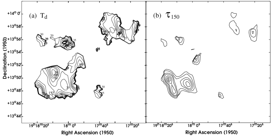
Figure 2: Dust temperature (T_d) and optical depth ($\tau_{150}$) distribution for the region around IRAS 19181+1349. (a) Temperature distribution. The contours are at the levels of 50, 40, 35, 30, 25, 20 and 15 K. (b) Optical depth distribution. The contours are at 90, 70, 50, 30, 20, 10 and 5% of the peak value which is 0.1.

The HIRES processed maps of IRAS 19181+1349 in the four IRAS bands, derived from the survey data are shown in Fig. 3. In HIRES maps also the source is resolved at all four wavelengths. It shows two components at 12 and 25 $\mu$m but at 60 and 100 $\mu$m only one component is seen. However, as seen from Table 1, even at 60 and 100 $\mu$m the source is extended with FWHM of $1\aas@@fstack{\prime}3\times 2\aas@@fstack{\prime}1$ and $2\aas@@fstack{\prime}3\times 3\aas@@fstack{\prime}1$ respectively as compared to the resolution of $1\aas@@fstack{\prime}1\times 1\aas@@fstack{\prime}6$ and $2\aas@@fstack{\prime}0\times 2\aas@@fstack{\prime}3$.

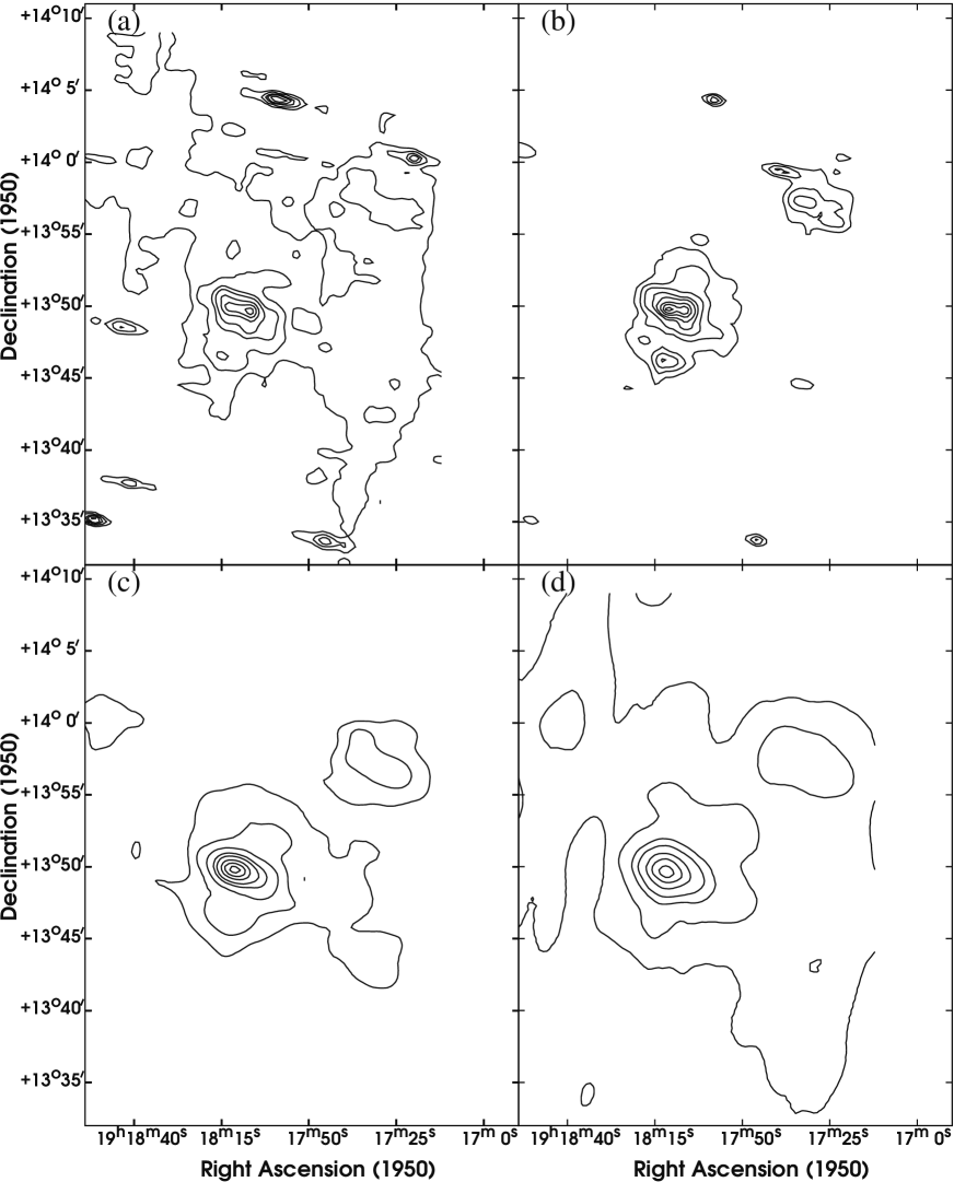
Figure 3: The HIRES processed intensity maps of the region around IRAS 19181+1349 at (a) 12 $\mu$m, (b) 25 $\mu$m, (c) 60 $\mu$m and (d) 100 $\mu$m. The contour levels are at 0.90, 0.70, 0.50, 0.30, 0.20, 0.10, and 0.05 of the peak intensity for 12 $\mu$m; for other wavelengths, besides these there are additional contours at 0.025 of the peak. The peak intensities are 26.4, 181, 1580 and 1090 Jy arcmin^-2 at 12, 25, 60 and 100 $\mu$m respectively.

Maps generated from ISOCAM images in the seven bands are shown in Fig. 4. The images in the SW filters have been physically shifted such that the positions of the main peaks in these images coincide with the respective positions in the LW filters. This was done to correct for the lens wheel jitter. This procedure has also been followed for the SW images of the other two sources. The required shift is $\sim 20\arcsec$. It can be seen from this figure that IRAS 19181+1349 consists of multiple components in all the filters. However the secondary peaks in the two SW filters do not appear in the LW filters and therefore do not seem to be associated with the IRAS source. The components in the LW filters can be divided into two groups separated by $\sim 1\aas@@fstack{\prime}5$, mainly in the E–W direction. This feature is also seen at 12 and 25 $\mu$m in the HIRES maps and at 210 $\mu$m in the TIFR map. Integrated flux densities of strong components are given in Table 3.

Table 3: Flux densities of sources in the ISOCAM images

IRAS	RA	Dec.	Flux Density in Jy∗
Source	(1950)	(1950)	SW2	SW6	LW4	LW5	LW6	LW7	LW8
			3.30 $\mu$m	3.72 $\mu$m	6.00 $\mu$m	6.75 $\mu$m	7.75 $\mu$m	9.62 $\mu$m	11.4 $\mu$m
			PAH		PAH		PAH		PAH
19181+1349	19 18 05.4	+13 49 22	–	–	0.81	1.34	2.6	–	1.29
	19 18 05.8	+13 50 32	0.10#	–	–	–	–	–	–
	19 18 06.8	+13 49 40	–	–	0.73	1.22	2.4	1.29	3.0
	19 18 07.6	+13 48 54	0.17#	0.19#	–	–	–	–	–
	19 18 11.2	+13 49 33	0.19	–	1.21	1.70	3.6	–	1.5
	19 18 12.2	+13 50 52	0.09	–	–	–	–	–	–
	19 18 12.5	+13 51 24	0.21	0.20	–	–	–	–	–
	19 18 12.6	+13 50 10	0.77	0.56	2.5	2.8	5.9	1.90	3.4
	19 18 13.0	+13 49 59	0.23#	0.13#	1.27#	1.51#	2.85#	–	–
	19 18 13.5	+13 49 24	–	–	0.78	0.96	2.0	–	–
20178+4046	20 17 53.3	+40 47 03	1.8	0.70	11.6	10.7	30.4	11.0	20.9
	20 17 55.0	+40 47 01	0.30#	–	2.7#	2.7#	7.5#	2.7#	4.6#
20286+4105	20 28 40.3	+41 05 14	0.71	0.23	4.4	4.8	11.5	3.5	6.3
	20 28 40.3	+41 05 45	0.25	0.13	3.1	3.3	7.8	1.90	2.8
	20 28 42.5	+41 05 44	0.20	0.12	2.9	2.4	3.5	1.21	1.50

^∗The flux densities have been integrated in a circle of $30\arcsec$ diameter around the peak except for those marked with ^# where the integration is done over an area of $18\arcsec\times 18\arcsec$ around the peak.

Figure 4: The maps of ISOCAM observations of the region around IRAS 19181+1349 at (a) 3.30 $\mu$m, (b) 3.72 $\mu$m, (c) 6.00 $\mu$m, (d) 6.75 $\mu$m, (e) 7.75 $\mu$m, (f) 9.62 $\mu$m, and (g) 11.4 $\mu$m. The contour levels are at 0.90, 0.70, 0.50, 0.30, 0.20, 0.10 and 0.05 of the peak intensity. The peak intensities are 19.5, 17.8, 36.5, 37.7, 70.2, 37.8 and 58.7 Jy arcmin^-2 at 3.30, 3.72, 6.00, 6.75, 7.75, 9.62 and 11.4 $\mu$m respectively.

3.2 IRAS 20178+4046

Around IRAS 20178+4046 an area of $\sim 30\arcmin\times 30\arcmin$ was scanned twice and the resulting deconvolved maps in the two far infrared bands are shown in Fig. 5. This source does not show multiple components in any of the two maps. It can be seen from Table 1 that the source is partly resolved.

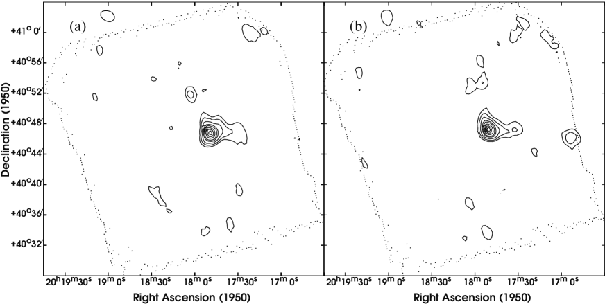
Figure 5: Same as figure 1 but for the region around IRAS 20178+4046. The peak intensities are 978 Jy arcmin^-2 at 150 $\mu$m and 589 Jy arcmin^-2 at 210 $\mu$m.

The dust temperature (T_d) and optical depth ($\tau_{150}$) maps for IRAS 20178+4046 are shown in Fig. 6. It is seen that the peak in optical depth occurs close to the peak in the intensity distributions. The temperature distribution shows two peaks separated by $2\aas@@fstack{\prime}4$. The total range in temperature is from 72 K to 21 K.

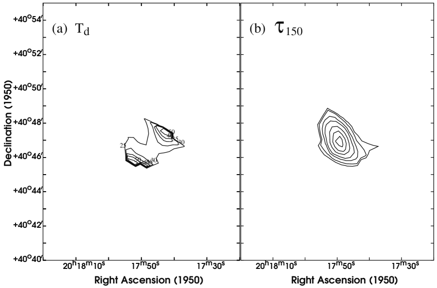
Figure 6: Same as figure 2 but for the region around IRAS 20178+4046. The temperature contours are at the levels of 50, 40, 35, 30 and 25 K and for the optical depth distribution the peak value is 0.038.

The HIRES processed maps of IRAS 20178+4046 in the four IRAS bands, derived from the survey data, are shown in Fig. 7. The central part of the source is not resolved in any of the IRAS bands, as seen from Table 1. However there is lower level extended emission in all the bands except at 25 $\mu$m.

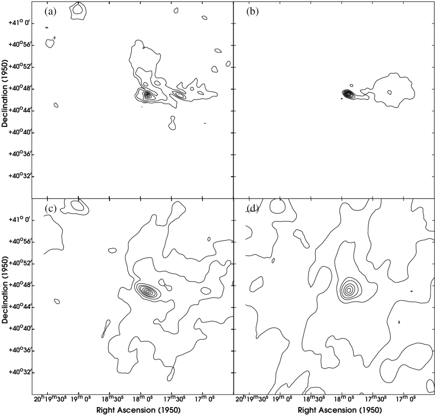
Figure 7: The HIRES processed intensity maps of the region around IRAS 20178+4046 at (a) 12 $\mu$m, (b) 25 $\mu$m, (c) 60 $\mu$m and (d) 100 $\mu$m. The contour levels are at 0.90, 0.70, 0.50, 0.30, 0.20, 0.10, 0.05 and 0.025 of the peak intensity; for 25 $\mu$m additional contour at 0.01 of the peak has been shown. The peak intensities are 89.7, 1490, 1110 and 737 Jy arcmin^-2 at 12, 25, 60 and 100 $\mu$m respectively.

Maps generated from the ISOCAM images in the seven bands are shown in Fig. 8. It can be seen from this figure that IRAS 20178+4046 consists of only one component in all the filters. The contours in all the LW filters are remarkably similar to each other, showing a lobe towards the south.

Figure 8: Same as figure 4 but for the region around IRAS 20178+4046. The peak intensities are 30.3, 15.2, 232, 214, 617, 239 and 505 Jy arcmin^-2 at 3.30, 3.72, 6.00, 6.75, 7.75, 9.62 and 11.4 $\mu$m respectively.

3.3 IRAS 20286+4105

Around IRAS 20286+4105 an area of $\sim 16\arcmin\times 30\arcmin$ was scanned twice and the resulting deconvolved maps in the two far infrared bands are shown in Fig. 9. As in the case of IRAS 20178+4046, this source also has only one component in both the bands. The source is resolved at 210 $\mu$m but at 150 $\mu$m it is unresolved. At 210 $\mu$m it shows an extension in the same direction (N-S) in which the source shows double structure in ISO maps (see later).

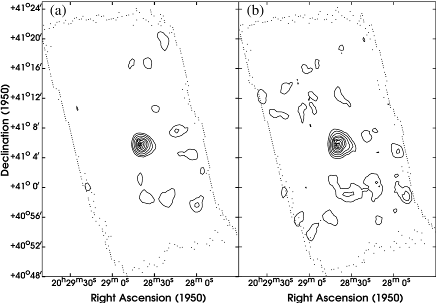
Figure 9: Same as figure 1 but for the region around IRAS 20286+4105. The peak intensities are 770 Jy arcmin^-2 at 150 $\mu$m and 402 Jy arcmin^-2 at 210 $\mu$m.

The dust temperature (T_d) and optical depth ($\tau_{150}$) maps for IRAS 20286+4105 are shown in Fig. 10. The dust in IRAS 20286+4105 is very much cooler (temperature range of 15 K to 25 K) than the other two sources. This is perhaps because the luminosity for this source is lowest (see Table 4). The peak in temperature occurs near the peak of the flux density distribution. However the peak in optical depth is shifted to the north by $\sim 1\arcmin$.

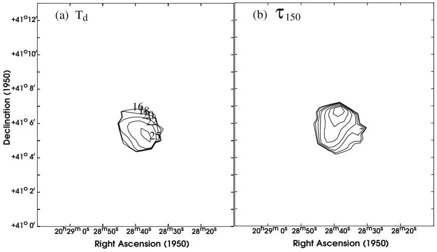
Figure 10: Same as figure 2 but for the region around IRAS 20286+4105. The temperature contours are at the levels of 25, 22, 20, 18 and 16 K and for the optical depth distribution the peak value is 0.042.

The HIRES processed maps of IRAS 20286+4105 in the four IRAS bands, are shown in Fig. 11. As seen from Table 1, the source is only resolved at 12 $\mu$m and partly resolved at 60 $\mu$m.

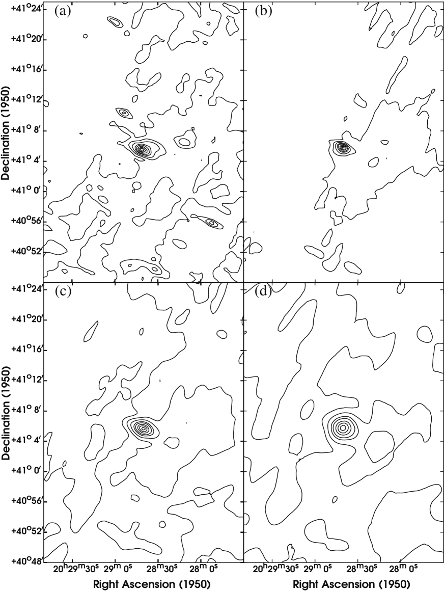
Figure 11: The HIRES processed intensity maps of the region around IRAS 20286+4105 at (a) 12 $\mu$m, (b) 25 $\mu$m, (c) 60 $\mu$m and (d) 100 $\mu$m. The contour levels are at 0.90, 0.70, 0.50, 0.30, 0.20, 0.10, 0.05 and 0.025 of the peak intensity. The peak intensities are 22.1, 175, 509 and 362 Jy arcmin^-2 at 12, 25, 60 and 100 $\mu$m respectively.

Maps generated from the ISOCAM images in the seven bands are shown in Fig. 12. It can be seen from this figure that IRAS 20286+4105 consists of two main components, separated along the N–S direction by $\sim 32\arcsec$ in all the filters. There is a third weaker component to the east. The structure in our maps (especially the SW maps) is very similar to the structure in the K band image of Comeron and Torra (2001).

Figure 12: Same as figure 4 but for the region around IRAS 20286+4105. The peak intensities are 9.9, 4.4, 77.4, 70.7, 183, 41.7 and 68.2 Jy arcmin^-2 at 3.30, 3.72, 6.00, 6.75, 7.75, 9.62 and 11.4 $\mu$m respectively.

4 Radiation Transfer Calculations

To understand the infrared emission from these sources radiation transfer calculations have been performed. The details of the basic radiation transfer scheme are given in Mookerjea et al. (1999). The geometry of the basic model is shown in Fig. 13a. Briefly, an internal radiation source, i.e., a star is surrounded by a spherically symmetric envelope of dust and gas mixture. The gas is assumed to be hydrogen and surrounds the star from the stellar surface itself. The dust is a mixture of astronomical silicates and graphite and there is an inner cavity of radius R_min which is devoid of dust. Two types of interstellar dust are considered; those with absorption and emission properties given by Draine & Lee (1984) (hereafter DL) and those with properties given by Mathis et al. (1983) (hereafter MMP) and the size distribution of the grains is taken to be a power law given by Mathis et al. (1977), viz. n(a)da $\propto$ a^-mda, with m = 3.5 and 0.01 $\mu$m $\leq$ a $\leq$ 0.25 $\mu$m; a is the radius of the grain. The envelope is surrounded by the interstellar radiation field (ISRF) taken from Mathis et al. (1983). The radial density distribution of the gas and dust has been taken to be a power law, i.e. n(r) $\propto$ r^-α with $\alpha$ = 0, 1 or 2. The radiation transport has been carried out using a program based on the code CSDUST3 (Egan et al. 1988). The parameters of the model are – inner radius of the dust cloud R_min, outer radius of the envelope R_max, $\alpha$, luminosity and temperature of the embedded star, relative abundance of the two types of dust, gas to dust ratio and the total radial optical depth at a selected wavelength ($\tau_{100}$ at 100 $\mu$m). The radiation transfer of Lyman continuum photons in gas is carried out in a consistent manner with that through the dust. The combination of the parameters is obtained which gives lowest $\chi^{2}$ to fit the observed SED. The scheme also gives the expected radio emission and the radial distribution of infrared emission. These have also been used to constraint the model. This basic scheme was used to model IRAS 20178+4046.

As ISOCAM maps of IRAS 20286+4105 show two main components in all the images, the radiation transfer calculations for this source were performed differently. Whereas the basic scheme of the radiation transfer is the same, it is assumed that there are two cores. Each core, with its own internal radiation source, is surrounded by a spherically symmetric envelope of dust and gas mixture. The type of dust (DL or MMP) and the silicate to graphite ratio is assumed to be the same for both cores. Total luminosity of the source is divided between the two cores in the ratio of their respective ISOCAM flux densities. The radiation transfer calculation is done for each core separately and the radiation emerging from each core is calculated. These cores are surrounded by another common shell, with the internal input radiation equal to the sum of the emerging radiation from each core. This common shell is surrounded by interstellar radiation field taken from Mathis et al. (1983). The radiation emerging from the inner boundary of this shell is the input at the outer boundary of the cores. The calculations are done iteratively. The geometry of the model is shown in Fig. 13b.

The radiation transfer calculations for IRAS 19181+1349 were performed in a cylindrical geometry with two embedded sources. This model has been described in Karnik and Ghosh (1999). An attempt was made to fit the SED as well as the radial profile of the intensities.

5 Discussion

5.1 IRAS 20178+4046

First we consider IRAS 20178+4046 which is the simplest of the three sources because it shows only one component in all the wavelength bands. We have constructed the SED of IRAS 20178+4046 using the flux densities from balloon-borne, IRAS and ISO observations, given in Tables 2 and 3, IRAS LRS data from Volks and Cohen (1989) and ground based observations of Faison et al. (1998). This SED is shown in Fig. 14a. In this figure, we have only shown ISOCAM flux densities in the continuum bands; PAH bands are treated separately. It can be seen that while there is general agreement between various observations, HIRES flux density at 12 $\mu$m is higher than IRAS LRS data as well as the data of Faison et al. (1998). This is because the HIRES flux density is integrated over 4$\arcmin$ dia and includes substantial amount of extended flux. Also, the flux densities of Faison et al. (1998) are lower than those of IRAS LRS as well as from ISO observations. This is because of the small aperture (9$\arcsec$) of Faison et al. (1998).

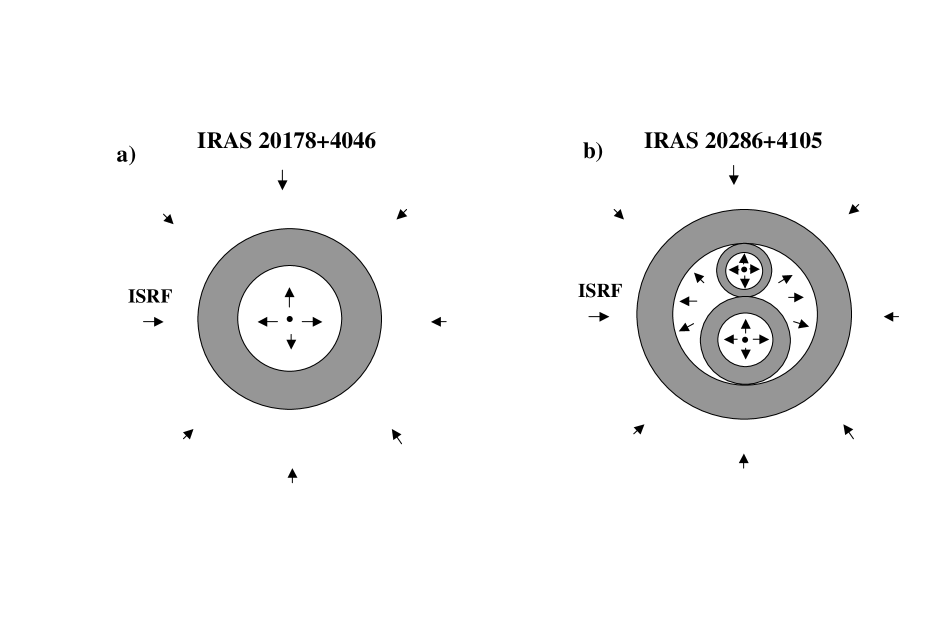
Figure 13: Geometry of the models for radiation transfer calculations; (a) for IRAS 20178+4046, (b) for IRAS 20286+4105. The dark circles in the centre represent embedded central stars and the grey areas the spherical shells of dust and gas. The white areas between the two contain only gas. For IRAS 20178+4046, the shell is heated from outside by the ISRF and from inside by the radiation from the embedded star. For IRAS 20286+4105, the radiation emerging out of the two inner gas-dust shells is combined and then used for heating the outer shell from inside. For more details refer to the text.

Figure 14: (a) SED of IRAS 20178+4046. Symbols are – circles - flux densities from balloon-borne observations and IRAS HIRES, squares - from ISOCAM maps, triangles - from ground based observations of Faison et al. (1998) and dotted line - from IRAS LRS. The solid curve shows the SED corresponding to the best fit model. (b) Same as (a) but for IRAS 20286+4105. (c) Same as (a) but for IRAS 19181+1349. The solid curve shows the best fit model for this source given in Karnik and Ghosh (1999).

The SED from the best fit radiation transfer model is shown in Fig. 14a. It can be seen that the calculated SED fits the observed one quite well. The parameters of the best fit model are given in Table 4. The luminosity corresponds to an O7 ZAMS star. The density distribution that fits best is, n(r) $\propto$ r^-2, the dust type is MMP and is dominated by silicates. The calculated angular sizes (deconvolved with the angular resolutions) are given in Table 1. It can be seen that the calculated angular sizes are consistent with the observed sizes. The calculated radio flux density at 6 cm is 72 mJy for a gas to dust ratio of 100. This can be compared with the observed flux density of 69 mJy by McCutcheon et al. (1991) and 65 mJy by Wilking et al. (1989). Density distribution (r^-2) is consistent with what is expected in the envelopes of young protostars from free fall models (see for example Shu et al. 1987). While it is true that the fitting of SED alone is not unique (Churchwell et al. 1990), in the present case angular distribution and radio flux are consistently modelled and therefore parameters of the model are on firmer footing.

5.2 IRAS 20286+4105

We have constructed the SED for IRAS 20286+4105 using the flux densities from balloon-borne, IRAS and ISO observations, given in Tables 2 and 3 and IRAS LRS data from Olnon et al. (1986). This SED is shown in Fig. 14b. For ISO observations we have combined the flux densities of two components (N and S); the third component toward the East gets weaker at longer wavelengths and therefore has not been included. It can be seen that there is good agreement between various observations.

The SED from the best fit radiation transfer model is shown in Fig. 14b. The calculated SED fits the observed SED quite well. The parameters of the best fit model are given in Table 4. Here the two cores are denoted as IRAS 20286+4105 N and IRAS 20286+4105 S. The luminosities of the two cores correspond to ZAMS stars of the type B0.5 (N) and B0-0.5 (S). The dust density distribution that fits best is, n(r) $\propto$ r^-1 and the dust type is again MMP and dominated by silicates. The radiation transfer model predicts negligible radio emission. No compact radio source has been observed in the field of IRAS 20286+4105. McCutcheon et al. (1991) see an extended feature at 6 cm and according to them the association of radio continuum with IRAS 20286+4105 is not clear. Similarly Wendker et al. (1991) see radio emission from IRAS 20286+4105 as a small density enhancement on a large ridge. Thus the model is consistent with radio observations. The flatter dust density distribution, as compared to IRAS 20178+4046, suggests that IRAS 20286+4105 is relatively more evolved system.

Table 4: Parameters^∗ for the best fit radiation transfer models

Source	Rmax	Rmin	L	$\alpha$	$\tau_{100}$	Dust Type	fSilicate
	(pc)	(pc)	(104 L☉)
20178+4046	3.40	0.077	9.5	2	0.12	MMP	0.76
20286+4105 N	0.24	0.022	1.2	1	0.11	MMP	0.65
20286+4105 S	0.32	0.022	2.3	1	0.11	MMP	0.65
20286+4105 Outer	3.02	1.12	3.5	1	0.025	MMP	0.65
19181+1349	1.8	0.03, 0.01	62, 63	0	0.10	DL	0.80

^∗The scheme of calculation for IRAS 19181+1349 is different from that of other sources. Therefore some of the parameters are not directly comparable.

5.3 IRAS 19181+1349

The SED for IRAS 19181+1349 using the flux densities from balloon-borne, IRAS and ISO observations, is shown in Fig. 14c. As was mentioned earlier, maps of IRAS 19181+1349 show multiple components in all the images. For this source we have used the flux density within 5$\arcmin$ of the main peak such that the contribution from multiple sources is included.

The SED for IRAS 19181+1349 was analyzed by Karnik and Ghosh (1999) using a model with two embedded sources in a cylindrical geometry. An attempt was made to fit the SED as well as radial profile of the intensities. The best fit to the SED is shown in Fig. 14c. The parameters of that model are given in Table 4. The prefered dust density distribution (r⁰) suggests that IRAS 19181+1349 is very evolved system.

5.4 PAH emission

As seen from Table 3, the emission in PAH bands is generally higher as compared to the neighbouring bands. We have derived line fluxes in the PAH bands from the flux densities given in Table 3. For this, we have subtracted the continuum flux density taken from the neighbouring filter; SW6 (3.72 $\mu$m) for 3.30 $\mu$m band, LW5 (6.75 $\mu$m) for 6.2 and 7.7 $\mu$m bands and LW7 (9.6 $\mu$m) for 11.3 $\mu$m band; and mutiplied by the filter bandwidth. This procedure will lead to an overestimation for the 11.3 $\mu$m PAH feature because the continuum given by LW7 is underestimated due to silicate absorption. The band fluxes and the band ratios are given in Table 5. It is seen that the strongest PAH feature is the one at 7.7 $\mu$m whereas the feature at 6.2 $\mu$m is absent in most of the cases. We have also given the range of band ratios obtained by Roelfsema et al. (1996) using ISO Short Wavelength Spectrometer (SWS) for six compact H ii and the average value of line ratios from typical H ii regions from Cohen et al. (1989). It is seen that the band ratios obtained by us are consistent with the values of Roelfsema et al. (1996) for three of the four features observed by us. However they are different from the values of Cohen et al. (1989) for typical H ii regions. For example, the ratio of 7.7 $\mu$m and 3.3 $\mu$m features varies from 18 to 52 in our data as compared to 17 to 73 in those of Roelfsema et al. (1996), but the average value of Cohen et al. (1989) is 7. This shows that there is a difference in the PAH emission by compact H ii regions and other H ii regions. However, we can not understand the near absence of the 6.2 $\mu$m PAH band in our observations especially as both, the 6.2 $\mu$m feature and the strongest observed feature at 7.7 $\mu$m arise from C-C stretching and have been found to be strongly correlated (Cohen et al. 1989).

Table 5: PAH band fluxes for the sources in ISOCAM images

IRAS	RA	Dec.	Band Fluxa (10-11 erg cm-2 s-1)				PAH Band Ratios
Source	(1950)	(1950)	3.3 $\mu$m	6.2 $\mu$m	7.7 $\mu$m	11.3 $\mu$m	6.2/3.3	7.7/3.3	11.3/3.3
19181+1349	19 18 05.4	+13 49 22	–	–	9.8	–	–	–	–
	19 18 06.8	+13 49 40	–	–	9.1	5.2	–	–	–
	19 18 11.2	+13 49 33	–	–	14.4	–	–	–	–
	19 18 12.5	+13 51 24	0.06	–	–	–	–	–	–
	19 18 12.6	+13 50 10	1.16	–	23	4.6	–	20	3.9
	19 18 13.0	+13 49 59	0.55	–	10.1	–	–	18	–
	19 18 13.5	+13 49 24	–	–	7.9	–	–	–	–
20178+4046	20 17 53.3	+40 47 03	6.1	7.6	149	30	1.25	25	5.0
	20 17 55.0	+40 47 01	–	–	36	5.8	–	–	–
20286+4105	20 28 40.3	+41 05 14	2.6	–	51	8.5	–	19	3.2
	20 28 40.3	+41 05 45	0.66	–	34	2.6	–	52	4.0
	20 28 42.5	+41 05 44	0.44	4.2	8.3	0.91	9.5	19	2.1
Compact H ii							3.4 – 22	7 – 44	2.9 – 6.7
regionsb
Typical H ii							4.0	7	2.3
regionsc

^aBand fluxes have been caculated after subtracting the continuum defined by the neighbouring filter as given in the text
^bThe flux ratios for compact H ii regions from Roelfsema et al. (1996)
^cThe flux ratios for typical H ii regions from Cohen et al. (1989)

In addition, an attempt has been made to generate the spatial distribution of emission in individual PAH features for the regions imaged by ISOCAM filters. The PAH emission maps have been generated by subtracting out the expected continuum emission. The spectrally local continuum emission has been estimated by linear interpolation or extrapolation using the neighbouring ISOCAM filters (viz., LW5 & LW7 for the features at 7.7 $\mu$m and 11.3 $\mu$m features; LW5 & SW6 for the features at 3.3 $\mu$m and 6.2 $\mu$m). Generally the above method has been successful, except for the case of 3.3 $\mu$m feature for IRAS 20178+4046 and IRAS 20286+4105. The failure of the latter cases is attributed to a large ratio ($\sim$ 15) of intensities between 6.75 $\mu$m and 3.72 $\mu$m, making linear extrapolation a suspect. In these cases the measured intensities in the nearest filter (SW6) itself have been used as an estimate of the local continuum.

The spatial distribution of emission in individual PAH features is found to be diffuse and widespread in nature. However, they qualitatively (morphologically) resemble the isophotes of total emission in the corresponding ISOCAM filters (i.e. uncorrected for the continuum), which have been presented in figures 4, 8 and 12. Hence these are not presented here. Instead, some quantitative results are presented. The total emission in the individual PAH features from the imaged regions of IRAS 19181+1349, 20178+4046 and 20286+4105 are tabulated in Table 6.

Table 6: Total emission in individual PAH features extracted from ISOCAM data

PAH	Total emission in the PAH feature
feature	erg sec-1 cm-2
	IRAS 19181+1349	IRAS 20178+4046	IRAS 20286+4105
3.3 $\mu$m	1.56 $\times 10^{-9}$	1.15 $\times 10^{-10}$	5.20 $\times 10^{-11}$
6.2 $\mu$m	–	3.44 $\times 10^{-10}$	–
7.7 $\mu$m	6.03 $\times 10^{-9}$	4.01 $\times 10^{-9}$	1.56 $\times 10^{-9}$
11.3 $\mu$m	7.45 $\times 10^{-10}$	9.62 $\times 10^{-10}$	3.60 $\times 10^{-10}$

Considering that the ratios of emission in the individual PAH features may contain information about their excitation mechanisms, these have been computed on pixel-by-pixel basis for the three sources considered here. The determination of these ratios have been restricted to regions with sufficient signal strengths in relevant PAH features. The summary of these ratios are presented in Table 7.

The scatters in the values of the feature ratios (see the standard deviations) is not measurement noise but represent their genuine spatial variation. This implies different physical conditions around each of the star forming regions which differentially affect the exciting mechanisms of individual PAH features. Whereas the mean ratios are similar for the regions IRAS 20178+4046 and 20286+4105, the values for the region IRAS 19181+1349 differ significantly. This may be related to their evolutionary stages, which is also indicated by the conclusions from the radiative transfer modelling (see Sect. 4.1.3; viz., the power law index of radial density distribution is flattest for IRAS 19181+1349, indicating it to be the most evolved source).

Table 7: Distribution of PAH feature ratios for the ISO images

IRAS	$I_{11.3}$/$I_{7.7}$	$I_{7.7}$/$I_{6.2}$	$I_{7.7}$/$I_{3.3}$
Source
19181+1349	0.30$\pm$0.39∗	–	23.2$\pm$11.8∗
	(1024)∗∗		(476)∗∗
20178+4046	0.84$\pm$0.40	14.7$\pm$8.3	19.9$\pm$14.0
	(289)	(199)	(143)
20286+4105	1.07$\pm$0.64	–	13.4$\pm$11.7
	(256)		(145)

^∗mean $\pm$ std. dev.
^∗∗(sample size : # of pixels)

6 Conclusions

We have mapped two ultracompact H ii regions and one molecular clump simultaneously in two far infrared bands using 1 m TIFR balloon-borne telescope. Using the maps from the balloon-borne observations, maps of dust temperature and optical depth have been obtained. We have also imaged the central $3\arcmin\times 3\arcmin$ regions of these sources in seven mid infrared bands using ISOCAM instrument of ISO. IRAS HIRES processed data have also been obtained for these sources in the four IRAS bands. There are certain similarities between various maps of the sources. Using the flux densities in all the 13 bands, as well as any other available data, SEDs have been constructed. Radiation transfer calculations have been done for the three sources with different geometries.

All the maps of IRAS 20178+4046 consist of mainly one source, with a lobe seen in the ISOCAM maps. This source has been modelled with a single core and excellent fit has been obtained to the SED, radio flux and angular sizes. The dust density distribution which gives best fit to the data is of the form r^-2 and the dust is dominated by silicates.

While the IRAS HIRES and TIFR maps of IRAS 20286+4105 consist of one source, ISOCAM maps show three sources at shorter wavelengths and two at longer wavelengths. This source has been modelled with two cores and excellent fit has been obtained to the SED along with consistency with radio observations. Dust in IRAS 20286+4105 has been found to be coolest. The dust density distribution which gives best fit to the data is of the form r^-1 and the dust is dominated by silicates.

The maps of IRAS 19181+1349 show multiple sources in all wavelengths. Hot spots have been found at positions away from the intensity peaks. Radiation transfer calculations for this source have been done in cylindrical geometry with two cores. The dust distribution which gives best fit to the data is the one with uniform density i.e. r⁰ and the dust is dominated by silicates.

The differing density distributions tend to imply that IRAS 20178+4046, 20286+4105 and 19181+1349 are in progressive order of their evolutionary stage.

Fluxes in four PAH bands have been obtained from the ISOCAM images. Ratios of the emission in different PAH bands have been obtained. Whereas two out of the three ratios have been found to be similar to the ratios obtained for other compact H ii regions the third ratio is quite different. Also, the band ratios for compact H ii regions have been found to be different from those for general H ii regions. Spatial distribution of PAH emission has been obtained and found to be diffuse and widespread.

- (1) Aumann, H.H., Fowler, J.W., & Melnyk, M. 1990, AJ, 99, 1674
- (2) Bronfman, L., Nyman, L.-A & May, J. 1996, A&AS, 115, 81
- (3) Casoli, F., Dupraz, C., Gerin, M., et al. 1986, MNRAS, 228, 43
- (4) Caswell, J.L., Murray, J.O., Roger, R.S., et al. 1975, A&A, 45, 239
- (5) Caswell, J.L., Vaile, R.A., Ellingsen, S.P., et al. 1995, MNRAS, 272, 96
- (6) Churchwell, E., Wolfire, M.G., & Wood, D.O.S. 1990, ApJ, 354, 247
- (7) Codella, C., Felli, M., & Natale, V. 1996, A&A, 311, 971
- (8) Cohen, M., Tielens, A.G.G.M., Bregman, J., et al. 1989, ApJ, 341, 246
- (9) Comeron, F., & Torra, J. 2001, A&A, 375, 539
- (10) Draine, B.T., & Lee, H.M. 1984, ApJ, 285, 89
- (11) Egan, M.P., Leung, C.M., & Spagna, G.F. 1988, Comput. Phys. Commun., 48, 271
- (12) Faison, M., Churchwell, E., Hofner, P., et al. 1998, ApJ, 500, 280
- (13) Forster, J.R., & Caswell, J.L. 1989, A&A, 213, 339
- (14) Ghosh, S.K., Iyengar, K.V.K., Rengarajan, T.N., et al. 1988, ApJ, 330, 928
- (15) Ghosh, S.K., Iyengar, K.V.K., Rengarajan, T.N., et al. 1989a, ApJS, 69, 233
- (16) Ghosh, S.K., Iyengar, K.V.K., Rengarajan, T.N., et al. 1989b, ApJ, 347, 338
- (17) Ghosh, S.K., Iyengar, K.V.K., Rengarajan, T.N., et al. 1990, ApJ, 353, 564
- (18) Ghosh, S.K., Mookerjea, B., Rengarajan, T.N., et al. 2000, A&A, 363, 744
- (19) Gull, S.F., & Daniell, G.J. 1978, Nature, 272, 686
- (20) IRAS Catalogs and Atlases 1988, The Joint Science Working Group, (Washington, DC : US Government Printing Office)
- (21) ISOCAM Observer’s Manual 1994, ISO Science Operations Team, (ESA/ESTEC, Noordwijk, The Netherland)
- (22) Karnik, A.D., & Ghosh, S.K. 1999, J. Astrophys. Astr., 20, 23
- (23) Karnik, A.D. 2000, Ph. D. Thesis, Univ. Bombay
- (24) Kurtz, S., Churchwell, E., & Wood, D.O.S. 1994, ApJS, 91, 659
- (25) Kurtz, S.E., Watson, A.M., Hofner, P., & Otte, B. 1999, ApJ, 514, 232
- (26) Mathis, J.S., Mezger, P.G., & Panagia, N. 1983, A&A, 128, 212
- (27) Mathis, J.S., Rumpl, W., & Nordsieck, K.H. 1977, ApJ, 217, 425
- (28) Mehringer, D.M., Goss, W.M., & Palmer, P. 1995, ApJ, 452, 304
- (29) McCutcheon, W.H., Dewdney, P.E., Purton, C.R., & Sato, T. 1991, AJ, 101, 1435
- (30) Molinari, S., Brand, J., Cesaroni, R., et al. 1996, A&A, 308, 573
- (31) Mookerjea, B., Ghosh, S.K., Karnik, A.D., et al. 1999, ApJ, 522, 285
- (32) Mookerjea, B., Ghosh, S.K., Rengarajan, T.N., Tandon, S.N., & Verma, R.P. 2000, AJ, 120, 1954
- (33) Odenwald, S.F. 1989, AJ, 97, 801
- (34) Odenwald, S.F., & Schwartz, P.R. 1989, ApJ, 345, L47
- (35) Olnon, F.M., Raimond, E., & IRAS Science Team, 1986, A&AS, 65, 607
- (36) Palagi, F., Cesaroni, R., Comoretto, G., et al. 1993, A&AS, 101, 153
- (37) Roelfsema, P.R., Cox, P., Tielens, A.G.G.M., et al. 1996, A&A, 315, L289
- (38) Shepherd, D.S., & Churchwell, E. 1996, ApJ, 457, 267
- (39) Shu, F.H., Adams, F.C., & Lizano, S. 1987, ARA&A, 25, 23
- (40) Verma, R.P., Rengarajan, T.N., & Ghosh, S.K. 1993, Bull. Astr. Soc. India, 21, 489
- (41) Verma, R.P., Ghosh, S.K., Karnik, A.D., Mookerjea, B., & Rengarajan, T.N. 1999a, Bull. Astr. Soc. India, 27, 159
- (42) Verma, R.P., Ghosh, S.K., Karnik, A.D., Mookerjea, B., & Rengarajan, T.N. 1999b, in The Universe as seen by ISO, ed. P. Cox & M.F. Kessler (ESA SP–427), 775
- (43) Volk, K., & Cohen, M. 1989, AJ, 98, 931
- (44) Wilking, B.A., Mundy, L.G., Blackwell, J.H., & Howe, J.E. 1989, ApJ, 345, 257
- (45) Wood, D.O.S., & Churchwell, E. 1989, ApJ, 340, 265
- (46) Zoonematkermani, S., Helfand, D.J., Becker, R.H., et al. 1990, ApJS, 74, 181