High-Resolution CHANDRA Spectroscopy of tau Scorpii: A Narrow-Line X-ray Spectrum From a Hot Star

Abstract

Long known to be an unusual early-type star by virtue of its hard and strong X-ray emission, $\tau$ Scorpii poses a severe challenge to the standard picture of O-star wind-shock X-ray emission. The Chandra HETGS spectrum now provides significant direct evidence that this B0.2 star does not fit this standard wind-shock framework. The many emission lines detected with the Chandra gratings are significantly narrower than what would be expected from a star with the known wind properties of $\tau$ Sco, although they are broader than the corresponding lines seen in late-type coronal sources. While line ratios are consistent with the hot plasma on this star being within a few stellar radii of the photosphere, from at least one He-like complex there is evidence that the X-ray emitting plasma is located more than a stellar radius above the photosphere. The Chandra spectrum of $\tau$ Sco is harder and more variable than those of other hot stars, with the exception of the young magnetized O star ${\theta}^{1}$ Ori C. We discuss these new results in the context of wind, coronal, and hybrid wind-magnetic models of hot-star X-ray emission.

1 Introduction

The surprising discovery of X-ray emission from OB stars by the Einstein satellite in the late 1970s (Harnden et al. 1979; and anticipated by UV superionization observations [Cassinelli & Olson 1979]) is now a 25-year-old mystery. Because magnetic dynamos and the associated coronal X-rays were not believed to exist in hot stars, alternative models have been sought since the discovery of X-rays from hot stars. Most of these center on some type of wind-shock mechanism that taps the copious energy in the massive radiation-driven winds of hot stars (Lucy & Solomon 1970; Castor, Abbott, & Klein 1975, hereafter CAK). Wind-shock models, especially the line-force instability shock model (Owocki, Castor, & Rybicki 1988; Feldmeier, Puls, & Pauldrach 1997; Feldmeier et al. 1997), have become the favored explanations for the observed OB star X-ray properties.

However, various pieces of evidence have recently emerged indicating that magnetic fields exist on some hot stars (Henrichs et al. 2000; Donati et al. 2001, 2002). There is also mounting evidence that the standard wind-shock scenario is inadequate for explaining the observed levels of X-ray production in many B stars (Berghöfer & Schmitt 1994; Cohen, Cassinelli, & MacFarlane 1997a; Cohen, Cassinelli, & Waldron 1997b), and perhaps in some O stars as well (Schulz et al. 2001; Waldron & Cassinelli 2001; Miller et al. 2002), leading to a revival in the idea that some type of dynamo mechanism might be operating on hot stars. Theoretical investigations of magnetized OB stars have followed (Charbonneau & MacGregor 2001; MacGregor & Cassinelli 2002), including studies of hybrid wind-magnetic models (Babel & Montmerle 1997; ud-Doula & Owocki 2002; Cassinelli et al. 2002).

Discriminating between the two broad pictures of X-ray emission in hot stars (magnetic coronal vs. wind shock) has been very difficult during the era of low-resolution X-ray spectroscopy. But with the launch of Chandra in 1999, a new, high-resolution window has opened, and we can now apply quantitative diagnostics in our attempts to understand the high-energy mechanisms operating in the most massive and luminous stars in our galaxy.

Coronal heating mechanisms are complex and, even in our own Sun, not fully understood. Their possible application to hot stars is certainly not clear, even in those hot stars for which magnetic fields have been detected. However, we can assume that any type of coronal X-ray-production mechanism involves the confinement of relatively stationary hot plasma near the photosphere. This is in contrast to wind shocks, which, whatever their nature (and many different specific models have been proposed), involve low-density hot plasma farther from the photosphere and moving at an appreciable velocity. This broad dichotomy naturally leads to several possible observational discriminants that might be implemented using high-resolution X-ray spectroscopy. These include the analysis of line widths (or even profiles), which could reflect Doppler broadening from the bulk outflow of winds (which in normal OB stars have terminal velocities of up to 3000 km s^-1) and emission-line ratios that are sensitive to density, the local radiation field, or (unfortunately) in some cases, both. There are numerous other spectral diagnostics available, including temperature-sensitive line ratios, spectral signatures of wind absorption, time variability of individual lines, and differential emission measure (DEM) fitting (multiline plus continuum global spectral modeling of X-ray emission from plasma with a continuous distribution of temperatures). All of these can be useful for determining the physical properties of the hot plasma on OB stars, and, ultimately for constraining models, but none can provide the same level of direct discrimination between the wind-shock and coronal scenarios as line profiles and ratios.

In this paper we report on the very high signal-to-noise, high-resolution Chandra HETGS spectrum of the B0.2 V star $\tau$ Sco. We chose to observe this particular hot star because it is one of the most unusual single hot stars, with indications already from various low-resolution X-ray observations that its X-ray properties are extreme and present a severe test to the standard wind-shock scenario. As such, it makes an interesting contrast to the five single O stars that have been observed at high resolution with Chandra and XMM up to this point. In fact, some of the unusual properties of $\tau$ Sco (discussed below in §3) have already inspired the development of alternate models of X-ray production, notably including the “clump infall” model of Howk et al. (2000). In this scenario overdense regions condense out of the wind, and the reduced line force due to the increased optical depth in the clumps results in these clumps falling back toward the star, generating strong shocks via interactions with the outflowing mean wind.

2 Observations

The data presented in this paper were taken between 2000 September 17 and 18, over two different Chandra orbits, with an effective total exposure time of 72 ks. We used the ACIS-S/HETGS configuration and report on the medium-energy grating (MEG) and high-energy grating (HEG) spectra, although we concentrate primarily on the MEG 1st order spectrum, which contains a total of 19348 counts (while the HEG 1st order spectrum has 5230 total counts). We extracted and analyzed the spectra with CIAO tools (Version 2.1.2), including the SHERPA model-fitting engine. We used the CALDB libraries, Version 2.6, and the OSIP files from 2000 August to build auxiliary response files and grating response matrices. We fit line-profile models using SHERPA, but astrophysical modeling of the spectral data took place outside of the CIAO environment with a custom non-LTE spectral synthesis code, described in section 5.2.

3 The Star, $\tau$ Sco

A member of the upper Sco-Cen association and a Morgan and Keenan system standard, the B0.2 V star $\tau$ Sco has been the subject of much study over the past several decades. At a distance of $132\pm 14$ pc (Perryman et al. 1997), this $m_{v}=2.8$ star is closer to the Earth than any hotter star. It has an effective temperature of $31,400\pm 300$ K and ${\rm{log}}~{}g=4.24\pm.03$ (Kilian 1992). UV observations show evidence for a wind with a terminal velocity of roughly 2000 km s^-1 (Lamers & Rogerson 1978). The mass-loss rate is difficult to determine because of the uncertain ionization correction, but it seems consistent with the theoretically expected value of $\dot{M}\approx 10^{-8}$ ${\rm M}_{\odot}\,$ yr ^-1 (calculations based on Abbott 1982). Published values based on UV absorption lines (e.g., Lamers & Rogerson 1978) and a recently determined upper limit based on IR emission lines (Zaal et al. 1999) are roughly half this value. These wind properties contrast with those of the prototypical early O supergiant $\zeta$ Pup, which has a mass-loss rate at least 100 times larger (because of its significantly larger luminosity). Chandra HETGS observations of $\zeta$ Pup were recently reported by Cassinelli et al. (2001), and clear signatures of the stellar wind (broadening and absorption effects) are seen in those data.

There are several unusual properties of $\tau$ Sco that might be relevant for our attempts to understand its X-ray properties: (1) It has a quite highly ionized wind, since the star is the coolest to show O VI in its COPERNICUS spectrum (Lamers & Rogerson 1978). (2) The wind is also stronger than normal for the star’s spectral type (Walborn, Parker, & Nichols 1995). (3) It has a very low $v_{rot}{\rm sin}i$ of $10\pm 5$ km s^-1 (Wolff, Edwards, & Preston 1982). (4) It shows unusual redshifted absorption of about 200 km s^-1 in some of the higher ionization UV lines (which also show much more extended blue absorption, as one would expect; Lamers & Rogerson 1978). (5) It is extremely young; perhaps being only 1 million years on the main sequence (Kilian 1994). (6) It shows unusually strong photospheric turbulence, as seen in optical and UV absorption lines (Smith & Karp 1979) and in the IR (Zaal et al. 1999).

In addition to these properties, it is already known from Einstein, ROSAT , and ASCA measurements that $\tau$ Sco has an unusually hard X-ray spectrum and a high X-ray luminosity (Cohen et al. 1997a, 1997b). It is this fact, along with the redshifted UV absorption (item 4 above), that prompted Howk et al. (2000) to develop their model of infalling clumps for $\tau$ Sco.

Many of these properties have been cited as evidence that $\tau$ Sco may not fit into the usual wind-shock picture of hot star X-ray production, or at least that its wind emission mechanism may be modified by the presence of a magnetic field or perhaps involve some other, less standard, wind-shock model. We address these issues in detail in the next sections.

4 The Data

The overall quality and richness of the Chandra HETGS data can be seen in the MEG first-order spectrum shown in Figure 1. There are numerous lines present in this high signal-to-noise spectrum, and they are much better separated than in any of the other hot stars thus far observed (because of the small wind broadening seen in $\tau$ Sco compared to these stars). In Figure 2 we show a portion of the MEG spectrum, centered on the neon Ly$\alpha$ line, compared with data from $\zeta$ Pup and Capella, a typical O supergiant wind source and a late-type coronal source, respectively. It is immediately obvious that $\tau$ Sco is superficially more similar to Capella than to $\zeta$ Pup.

To quantify the properties of the spectrum, we fitted every strong line with a simple model (Gaussian plus a polynomial for the nearby continuum), providing values of the line flux, characteristic width, and central wavelength. We employed the appropriate spectral response matrices in these fits, so the derived line widths are intrinsic and do not include instrumental broadening. When there was sufficient signal, we fit the MEG and HEG data simultaneously. These results are summarized in Table 1, with the several strongly blended spectral features listed in Table 2. The astrophysical analysis of these data is presented in §5.

Time variability properties of $\tau$ Sco are also of interest in discriminating between the two primary X-ray-production mechanisms. In Figure 3 we show a lightcurve formed of all the photons in the -1,-2,-3,+3,+2,+1 orders of both the MEG and the HEG. The bins are 1000 seconds in length. The data are not consistent with a constant source (at $P>99.99$ %), but no large flare-type events, with a sudden increase in flux followed by a gradual decline back to the basal level, are seen. The standard deviation of the data is slightly less than 10 % of the mean. Only one individual line feature, the oxygen Ly$\alpha$ line near 19 Å, shows evidence of significant variability. Its lightcurve is shown in Figure 4. We tested other strong lines, and only the Fe XVII line at 15.01 Å shows even marginal variability.

5 The X-ray Diagnostics and Analysis

5.1 Line Widths

The emission lines of $\tau$ Sco are obviously narrow compared to the same lines observed in hot-star wind X-ray sources like $\zeta$ Pup, but how intrinsically narrow are they? Might they be no broader than thermal broadening would dictate? To answer these questions, we fitted Gaussian line models, convolved with the instrumental response function, so the width of the model Gaussian reflects the actual width of the emitted line. We do not know what actual line profile shape is warranted, but because the Gaussian model is simple and relatively general and the observed line broadening is not dramatic, we did not attempt to fit other profile shapes.

The line widths–half-width at half maximum (HWHM)–listed in Table 1 generally exceed by a factor of about 3 those expected from thermal broadening (assuming a temperature equal to that at which the emissivity for a given line peaks). In addition, fits we performed to Capella and AB Dor (both late-type coronal sources) using the same procedures found narrower lines (consistent with thermal broadening) than we found for $\tau$ Sco. In Figure 5 we show the Ne X line of $\tau$ Sco in the MEG, along with an intrinsically narrow line (Gaussian model with $\sigma=0$; i.e. a delta function) convolved with the instrumental response. The data clearly are broader than the model. We also note that some of the features in the spectrum are doublets. We generally fitted these with single-Gaussian models. In each case in which we fitted a doublet with a single-line model, the separation of the two components of the doublet was far less than the typical (and derived) line width. Thus the derived line widths using this procedure are only marginally elevated because of the blended doublet.

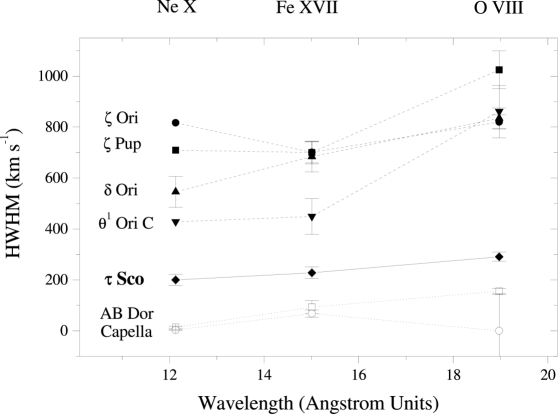
Figure 6: Derived line widths (HWHM) for three strong lines in seven stars: two stars representative of coronal sources (Capella and AB Dor: open symbols connected by dotted lines), $\tau$ Sco (filled diamonds and solid line), and four O stars (filled symbols and dashed lines), which are presumably wind X-ray sources.

The velocities of most of the lines in the HETGS spectrum of $\tau$ Sco are a few hundred km s^-1 (HWHM), which, while greater than the thermal velocity, is significantly less than the wind terminal velocity. The X-ray line velocities seen in $\tau$ Sco are thus larger than those in coronal sources and smaller than those in wind sources, a trend that is shown in Figure 6, and importantly, the velocities derived for the wind of $\tau$ Sco are significantly less than what would be seen if the X-ray-emitting gas had the same velocity distribution as the UV-absorbing gas.

The mean HWHMs of the strongest, unblended lines are roughly 300 km s^-1, or 15% of the terminal velocity of the wind of $\tau$ Sco (see Fig. 7). There is a slight trend of decreasing line width with wavelength, which is the opposite of what is seen in the O stars (Kahn et al. 2001; Waldron & Cassinelli 2001; Cassinelli et al. 2001; Miller et al. 2002). In the O stars, the trend of increasing line width with wavelength can be understood in terms either of temperature stratification (lower temperature plasma farther out in the wind, traveling at higher velocities) or an absorption effect (low energies are preferentially attenuated, so these lines tend to be broader because only photons from the outer wind, where velocities tend to be high, can escape). The lack of such a trend in $\tau$ Sco might be evidence of the lack of any wind continuum absorption effects on the observed spectral lines. The wind is expected to be optically thin down to $r\lesssim 1.5$ $R_{\mathchar 8707\relax}$ near 0.5 keV and effectively completely optically thin at photon energies of 1 keV and above.

5.2 Radiation-Sensitive Line Ratios

The He-like forbidden-to-intercombination line strength ratio is known to be sensitive to the local mean intensity of the UV radiation field (Gabriel & Jordan 1969; Blumenthal, Drake, & Tucker 1972; Waldron & Cassinelli 2001; Kahn et al. 2001). If the photospheric flux is strong enough, then electrons can be radiatively excited out of the metastable upper level of the forbidden line (${}^{3}S_{1}$) to the upper level of the intercombination line (${}^{3}P_{1,2}$), weakening the forbidden line and strengthening the intercombination line. Thus a measurement of the f/i ratio [using the more standard spectroscopic notation, $z/(x+y)$], potentially yields the radius of the X-ray emitting plasma (via sensitivity of the mean intensity to the dilution factor). This assumes that we know or can ignore limb darkening and other geometrical effects and that we know the UV luminosity of the star at the relevant wavelengths.

More traditionally, this line ratio has been used as a density diagnostic in coronal sources (where, because of the low temperature of the stars, very little UV radiation is present). Of course, in hot stars, this line ratio is still sensitive to density (via collisional excitation between the same two levels described above). However, the densities that would be required to explain the small observed f/i values are very large, while the radiation field requirements are much more reasonable.

In order to extract information from these line ratios, we model the oxygen, neon, magnesium, and silicon excitation/ionization using NLTERT, a non-LTE radiation transport and statistical equilibrium code (described in MacFarlane et al. 1993; MacFarlane, Cohen, and Wang 1994). We use a Kurucz model atmosphere, constrained by observational data in the spacecraft UV (relevant for O and Ne), but unconstrained by direct observation in the far-UV (Mg) and extreme-UV (EUV) (Si and S). We note that the model atmosphere fluxes are sensitive to the adopted temperature only in the EUV, in which a change of 1000 K can lead to about a factor of 2 change in emergent flux.

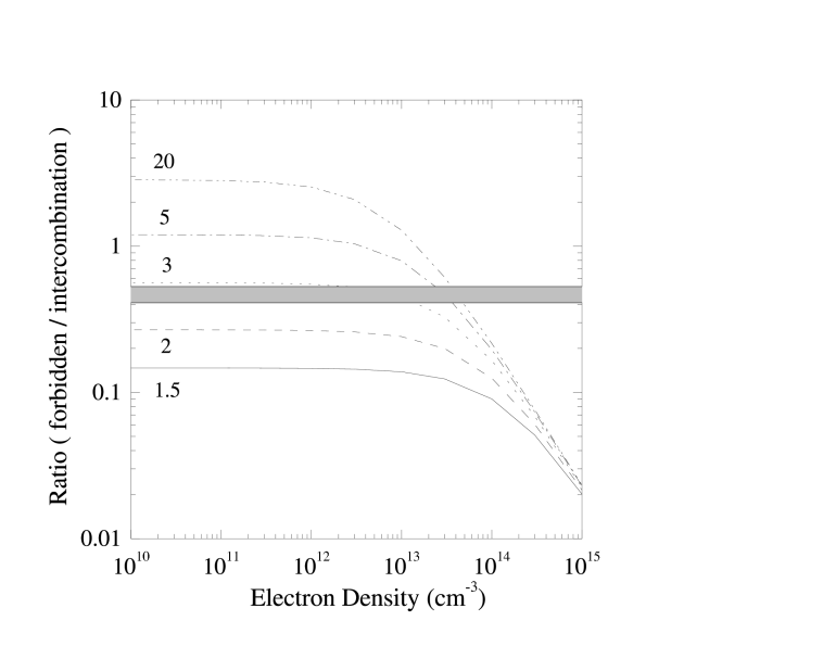
Figure 9: Calculation of the density and mean-intensity sensitivity of the f/i line ratio for Mg XI. Note that the sensitivity to the mean intensity enters via the distance from the photosphere. The distance of the plasma from the photosphere is indicated for each model in units of the stellar radius. The range from the data is indicated by the shaded area.

The He$\alpha$ line complexes are shown in Figure 8. When the metastable level is neither collisionally nor radiatively destroyed (i.e., the “low-density limit”), the forbidden lines tend to be about a factor of 3 stronger than the intercombination lines. We can see in the figure that the forbidden line is heavily affected in oxygen and neon, less so in magnesium, and less still in silicon. The S XV data are marginal, but are shown for the sake of completeness. In Figure 9 we show the results of our model calculation for He-like magnesium. Note that we model the effects of both radiation and collisions (i.e., showing both the radial sensitivity and the density sensitivity) in these calculations. Similar calculations were carried out for the He-like features for the other four species. The results of these calculations and the constraints they imply for the location of the X-ray emitting plasma are summarized in Table 3. The quoted errors on the determinations of the radii of line formation include statistical errors only. The uncertainties in the atmosphere model and the associated UV luminosity will certainly affect the results for Si XIII (and S XV) more than for the other three line ratios. For example, if the flux were actually twice as high as in the model atmosphere, then the lower limit to the radius of line formation would move out from $r=1.1$ $R_{\mathchar 8707\relax}$ to almost 1.5 $R_{\mathchar 8707\relax}$.

We also point out that, where other lines were present (primarily iron lines near the neon complex), we fitted them at the same time we fitted the He-like features, and upper limits to the nondetected forbidden lines were determined by fitting a Gaussian model with its centroid position fixed at the laboratory wavelength and its width fixed at the value derived for the corresponding He-like resonance line.

In general, it can be seen that most of these line ratio diagnostics are consistent with the X-ray emitting plasma being within several stellar radii of the photosphere. The oxygen and sulfur complexes do not really provide interesting constraints, as they are consistent with the X-ray emitting plasma being either right above the photosphere or far out in the wind flow. The neon ratio implies that the plasma giving rise to this complex is within a stellar radius of the photosphere, but confusion and blending with nearby iron lines may make this result somewhat less firm than the formal errors imply. The strongest constraints are provided by the Mg XI and Si XIII features. The Mg XI f/i ratio requires the X-ray emitting plasma be at least 1.6 $R_{\mathchar 8707\relax}$ above the photosphere (but no more than 1.9 $R_{\mathchar 8707\relax}$). The Si XIII f/i ratio indicates that the hotter plasma giving rise to this feature is closer to the star, a trend that is also seen in the O stars observed with Chandra (Waldron & Cassinelli 2001; Cassinelli et al. 2001; Miller et al. 2002).

Finally, we note that the intercombination line fluxes exceed the resonance line fluxes in the case of oxygen and neon. While the intercombination line strength is generally expected to be less than that of the resonance line in collisional plasmas, the observed G ratios ($(i+f)/r$) for these complexes are not inconsistent with a collisional plasma, since the enhanced intercombination line flux comes at the expense of the weakened forbidden line (Pradhan & Shull 1981).

5.3 Density-Sensitive Line Ratios

While the helium-like forbidden-to-intercombination ratios are sensitive to both density (via the collisional destruction of the ${}^{3}S$ level) and the local radiation field (through photoexcitation from the same level), we have argued in §5.2 that in hot stars like $\tau$ Sco, the ratio is dominated by radiative effects. This, of course, makes them relatively useless as density diagnostics, although, for He-like ions for which the forbidden line is strong, an upper limit can be placed on the density of the X-ray-emitting plasma (as well as on the local value of the mean intensity). The He-like complexes we observe imply upper limits of $n_{\rm e}\approx 10^{13}$ - $10^{14}$ cm^-3.

It is possible to determine an upper limit for the density via the Fe XVII 17.10-to-17.05 Å line ratio. The upper level of the 17.10 Å line is metastable, and so this ratio is density sensitive with a critical density of about $n_{e}\approx 10^{14}$ cm^-3 (Mauche, Liedahl, & Fournier 2001), but the energy spacing of this deexciting transition is larger than that for the He-like diagnostics, so that photoexcitation requires a photon with a wavelength below 400 Å. Thus, for all practical purposes, in a B star this diagnostic is not sensitive to photospheric UV photoexcitation. In the HETGS spectrum of $\tau$ Sco, we see the 17.10-to-17.05 Å ratio in the low-density limit. Thus there is no evidence for very dense ($n_{e}\gtrsim 10^{14}$ cm^-3) X-ray emitting plasma on $\tau$ Sco.

5.4 Line Centroids

In fitting the lines in the grating spectrum, we allowed the line centroid wavelength to be a free parameter. These results, along with line strengths and widths, are listed in Table 1. Although each individual line centroid is roughly consistent with the laboratory value of the wavelength, when taken as a whole, there is the potential to see an aggregate wavelength shift in the ensemble of lines. We calculated the weighted mean centroid velocity for the roughly two dozen strongest unblended lines and found a value of $v_{\rm centroid}=14\pm 61$ km s^-1 (see Fig. 10). The heliocentric correction actually shifts this number to the blue by about $-27$ km s^-1, making the heliocentric weighted-mean line centroid velocity $-13\pm 61$ km s^-1. Thus, there is no direct evidence for redshifted emission that might be expected from the shocking of infalling clumps, as in the Howk et al. (2000) model, which could be associated with the wind component that gives rise to the observed redshifted UV absorption. We cannot, however, rule out redshifted X-ray emission with net velocities of the order of 100 km s^-1.

5.5 Temperature Distribution in the Hot Plasma

We are deferring detailed DEM modeling of the global HETG spectrum to a future paper. The three-temperature MEKAL (Mewe, Kaastra, & Liedahl 1995) collisional equilibrium model that fitted the ASCA spectrum of this star (Cohen et al. 1997b), does an adequate job of matching the gross properties of the HETGS spectrum. Of course, with the vast increase in spectral resolution with Chandra, this model does not fit in detail. However, it is clear that a detailed, global fit to the spectrum will not drastically alter the results from the fit to the ASCA spectrum. One question left open by the analysis of the medium-resolution ASCA data is the extent to which the high-temperature component of the spectrum is present, in terms of both the overall emission measure of the hot component and the actual maximum plasma temperature.

We find no obvious evidence for plasma with temperatures above the 27 MK lower limit to the hottest temperature component that was found in the ASCA spectrum, and in fact, our detection of the S XV feature, which is relatively prominent in the ASCA spectrum, is quite marginal in the HETGS spectrum. This is perhaps not surprising, however, given the much lower detector effective area available with HETGS + ACIS-S compared to ASCA Solid-State Imaging Spectrometer.

We have made a rough assessment of the temperature distribution implied by the H-like to He-like line ratios from O, Ne, Mg, and Si. We modeled these ratios using the same NLTERT non-LTE ionization/excitation code (MacFarlane et al. 1993) that we used to model the He-like f/i ratios. The best-fit temperature for each of these ions can be determined from the observed line ratios under the assumption of coronal equilibrium. We found temperatures ranging from less than 3 MK for oxygen to slightly more than 10 MK for the silicon. This is in agreement with the expectations from the off-the-shelf collisional equilibrium codes, such as APEC (Smith et al. 2001), and it represents a wider temperature range than is seen in the O stars $\zeta$ Pup and $\zeta$ Ori based on this same diagnostic. Of course, the presence of a wide range of plasma temperatures is not surprising, and by itself is not a strong discriminant among the various physical models of X-ray production in hot stars.

Finally, the wavelength region between 10 Å and 12 Å contains several lines from high ionization stages of iron, including Fe XXIII at 11.02 Å and 11.74 Å and and Fe XXIV at 10.62 Å. The equilibrium temperatures of peak emissivity of these lines are roughly 20 MK (APED; Smith et al. 2001). These lines are quite strong in the spectrum of $\tau$ Sco. Of the other hot stars observed thus far with Chandra HETGS, only ${\theta}^{1}$ Ori C shows these features as strongly as does $\tau$ Sco. Thus, there is evidence in the Chandra spectrum of $\tau$ Sco for a not-inconsequential amount of very hot plasma, qualitatively confirming the earlier ASCA results, and demonstrating a similarity between $\tau$ Sco and ${\theta}^{1}$ Ori C that sets both of these young hot stars apart from the more standard O supergiants.

5.6 Time Variability

Active coronal sources, including pre-main-sequence stars, show frequent and strong flaring activity, often in conjunction with very high plasma temperatures (e.g., AB Dor: Linsky & Gagné 2001; pre-main-sequence stars: Montmerle et al. 2002). Wind-shock sources show very little variability, and whatever variability is seen has been interpreted as being stochastic and reflecting a Poisson statistical description of the number of individual sites of X-ray emission within the wind (Oskinova et al. 2001). Variability levels of 10%, as are seen in the Chandra spectra of $\tau$ Sco, could then be interpreted as an indication that there are roughly 100 individual sites of X-ray emission at any given time on this star. Of course, arguments about characteristic timescales (of, e.g., cooling), as well as the evolution of the physical properties of individual emission sites, have a bearing on the details of this interpretation.

Our detection of variability in the oxygen Ly$\alpha$ line at 18.97 Å, but in no other line, could indicate that the relatively cooler gas that gives rise to this feature has a more variable emission measure than do other lines, and thus O VIII might be present in fewer discrete sites within the X-ray emitting region, whether it is wind shocks or magnetically confined coronal plasma. It could, on the other hand, be an indication that the level of absorption by the overlying cool wind is variable. The long-wavelength lines like O VIII are the most likely lines to be subject to wind absorption. However, the expectation is that there is very little continuum absorption of the X-rays in a hot star like $\tau$ Sco, which has a relatively low-density wind. We note that there is enough signal in several other lines (Si XIII, Mg XI, several Fe XVII lines, for example) that variability at the level seen in the O VIII line would be detected if it were present. We also note that the time dependence of the variability in this line tracks the overall X-ray variability in the spectrum as a whole and also that the even longer wavelength lines of O VII and N VII do not have enough signal for any variability to be detected.

6 Discussion

The qualitative impression one gets from comparing the HETGS spectrum of $\tau$ Sco to that of other stars is that this early B star has more in common with late-type coronal X-ray sources than with early-type wind sources. This impression is borne out primarily in the analysis of the line widths. The emission lines are indeed narrow, although they are not as narrow as the same lines seen in Capella and AB Dor. The bulk flow velocities derived from these lines, while supersonic, are only 10% - 20% of the wind terminal velocity.

If embedded in a standard CAK wind, the X-ray-emitting regions would have to be within just a few tenths of a stellar radius from the photosphere based on the observed line widths. However, the He-like $f/i$ ratios put constraints on the proximity of the X-ray emitting plasma to the photosphere. These results are consistent with a height of 1$R_{\mathchar 8707\relax}$-2$R_{\mathchar 8707\relax}$ ($2{{R_{\mathchar 8707\relax}}}<r<3{{R_{\mathchar 8707\relax}}}$), and for Mg XI the plasma must be at least 1.6 $R_{\mathchar 8707\relax}$ above the photosphere. There is thus a contradiction, that would seem to imply the presence of hot plasma out to a few stellar radii above the surface of $\tau$ Sco, but moving with very small (but nonzero) line-of-sight velocity. This picture is inconsistent with standard wind-shock scenarios (which seem to apply to O supergiants like $\zeta$ Pup) in which hot plasma is embedded within the massive line-driven wind. Our data show lines far too narrow for this to be the case. A similar situation is seen in the O9.5 star $\delta$ Ori, though the emission lines in that star are significantly broader than what is seen in the spectrum of $\tau$ Sco (Miller et al. 2002).

It is also difficult, however, to reconcile these data with a generic, solar-type picture of magnetic X-ray activity, in which small magnetic loops confine plasma heated by magnetic reconnection and the deposition of mechanical energy. In this picture, the plasma would be closer to the UV-bright photosphere of $\tau$ Sco than can be accounted for by the observed $f/i$ value for magnesium. Furthermore, we see no evidence for coronal X-ray flaring in our data. It is conceivable that relatively stable, large scale magnetic loops could exist on the surface of $\tau$ Sco, with hot plasma confined at the tops of the loops, several stellar radii from the surface, but the standard picture of energetic, relatively small spatial scale magnetic activity, as seen in the sun, is not consistent with these observations of $\tau$ Sco.

One scenario that could explain the two primary results from the analysis of the Chandra HETGS spectrum of $\tau$ Sco is the “clump infall” model (Howk et al. 2000), which was put forward to explain the hard ASCA spectrum and the redshifted UV absorption features seen in this star. In this model it is assumed that density enhancements (“clumps”) form in the wind of a hot star. The authors explored the dynamics of such clumps under the combined influence of radiation driving, gravity, and wind drag. They found that for the parameters appropriate to $\tau$ Sco, such density enhancements stall at heights of several stellar radii, and fall back toward the star. A bow shock would develop around each clump, leading to strong shock heating and presumably hard X-ray emission. The infalling clumps then also explain the observed redshifted UV absorption features. Since the outflowing wind, when it passes through the shock front associated with one of these density enhancements, would be slowed by a factor of 4, this scenario provides a means for explaining the lack of strong line-broadening seen in our Chandra spectrum, and the heights at which these clumps stall are consistent with the He-like f/i ratios. It should be stressed, however, that Howk et al. (2000) present no specific mechanism for the condensation of these density enhancements out of the wind.

The relative youth of $\tau$ Sco (Kilian 1994) has suggested that a fossil magnetic field may be present in this star. The very low projected rotational velocity is also consistent with magnetic spin-down (or, of course, with a pole-on viewing angle). Recent modeling of radiation-driven winds in the presence of a dipole magnetic field (Babel & Montmerle 1997; Donati et al. 2002; ud-Doula & Owocki 2002) has suggested another scenario that may also be relevant for $\tau$ Sco and could explain the formation of density enhancements at several stellar radii in this star’s wind. The magnetically confined wind shock (MCWS) model predicts the confinement of the stellar wind by a strong enough dipole field and the subsequent shock heating of wind material trapped in the field and forced to collide at the magnetic equator. In the case of $\tau$ Sco, a field of less than 100 G is required to provide the necessary confinement (ud-Doula & Owocki 2002). This model has been successfully applied to ${\theta}^{1}$ Ori C (Donati et al. 2002), which is a very young O star with X-ray properties similar to those of $\tau$ Sco.

Dynamic simulations have shown that plasma in the post-shock region in the MCWS model can eventually fall back toward the star when it can no longer be supported by radiation pressure and magnetic tension (ud-Doula & Owocki 2002). By coupling this mechanism to the Howk et al. (2000) scenario, we may have a self-consistent, physical picture of the strong shock heating of wind plasma, in a nearly stationary equatorial zone, at a height of several stellar radii, with periodic infalling of material. We await dynamical simulations of this particular star in order to make quantitative comparisons with our observational data. In addition, synthesis of X-ray line profiles from the dynamical simulations would be very important, since it is not clear if the specific observed small line widths can be produced within this context.

The other properties we derived from the $\tau$ Sco HETGS spectrum can perhaps also be explained in this scenario of magnetic wind shock heating and confinement combined with the infall of density enhancements in the wind. The high plasma temperatures are naturally explained by the large shock velocities inherent in the collision between the fast stellar wind and the equatorial shocked disk (as well as with the infalling clumps).

The lack of very dense plasma argues against very dense coronal-type magnetic structures near the photosphere, although some level and type of coronal heating mechanism is certainly not ruled out. In fact, recent work (Charbonneau & MacGregor 2001; MacGregor & Cassinelli 2002) suggests that a dynamo mechanism could be operating in the interiors of normal OB stars and that if a means of bringing the dynamo-generated magnetic fields to the surface could be identified, then solar-type coronal activity on hot stars may be quite plausible. The modest time variability seen in the Chandra spectrum is more significant than that seen in O stars that are supposed to be wind X-ray sources. This variability level (rms variations at the 10% level) may simply be indicative of a relatively small number of sites of X-ray production on $\tau$ Sco as compared with O stars showing a more standard mode of wind-shock X-ray production (Oskinova et al. 2001), and no large flare events were seen in this observation of $\tau$ Sco (or in any of the earlier X-ray observations of this star). Therefore, any coronal model applied to $\tau$ Sco would need to explain the high temperatures (presumably with a strong dynamo mechanism of some sort) but also the absence of frequent strong flaring. In addition, such a coronal mechanism would need to explain the presence of bulk plasma velocities of several hundred km s^-1, along with at least some X-ray-emitting plasma a significant height above the surface of the star.

In summary, the unusual X-ray properties of $\tau$ Sco, elucidated in great detail for the first time by the superior spectral resolution of the Chandra HETGS, now require detailed dynamical modeling in order to test the viability of the MCWS model, deduce the role of clump infall, and test the alternate scenario of dynamo activity. However, we can say with certainty that the standard picture of numerous shocks embedded in a fast stellar wind cannot explain the narrow X-ray lines and the formation heights of several stellar radii of the very hot X-ray emitting plasma on this young hot star.

Figure 1: Combined MEG +1 and -1 order spectrum of $\tau$ Sco with lines labeled

Figure 2: Combined MEG +1 and -1 order spectra of Capella, $\tau$ Sco, and $\zeta$ Pup (top to bottom), centered on the region around the Ne X line at 12.13 Å.

Figure 3: X-ray light curve formed from the combined MEG +1 and -1 order counts, with 1000 second bins. The mean count rate is indicated by the dashed line. The hypothesis of a constant source can be rejected at a more than 99.99% confidence level.

Figure 4: X-ray light curve formed from the combined MEG +1 and -1 order counts in the O VIII line at 18.97 Å, with 10,000 s bins. The mean count rate is indicated by the dashed line. The hypothesis of a constant source can be rejected at a more than 99% confidence level.

Figure 5: MEG +1 and -1 order observation of the neon Ly$\alpha$ line (histogram) with an intrinsically narrow model (convolved with the instrument response). The fit to the data show a statistically significant line width.

Figure 7: HWHM for the strongest unblended lines in the HETGS spectrum of $\tau$ Sco. The best-fit linear function is indicated by the solid line with the 95 % confidence limits shown as dashed lines.

Figure 8: MEG +1 and -1 order data for the helium complexes of S XV, Si XIII, Mg XI, Ne IX, and O VII along with the best-fit models. Note that the error bars shown here (Sherpa’s “chi Gehrels” option) represent Poisson noise plus a constant. We used the Cash C statistic as our goodness-of-fit indicator, and this statistic does not make use of the formal errors.

Figure 10: Line centroids derived from fitting Gaussian models to the strongest lines in the HETGS spectrum. The dashed line indicates the weighted mean centroid velocity.

Table 1: Emission Lines in the HETGS Spectrum

Ion	$\lambda_{lab}$	$\lambda_{obs}$	Flux	Half-Width	Centroid Velocity	log $T_{\rm max-emiss}$
	(Å)	(Å)	($10^{-5}$ ph s-1 cm-2)	(km s-1)	(km s-1)	(K)
S XV	$5.0387\pm 0.002$	$\cdots$	$0.936^{+.270}_{-.235}$	$\cdots$	$\cdots$	7.1
S XV	$5.0631\pm 0.002$	$\cdots$	$0.464^{+.234}_{-.196}$	$\cdots$	$\cdots$	7.1
S XV	$5.1015\pm 0.002$	$\cdots$	$0.944^{+.268}_{-.234}$	$\cdots$	$\cdots$	7.1
Si XIV	$6.1821\pm 0.0003$	$6.1832\pm 0.0011$	$2.267^{+.199}_{-.188}$	$424^{+84}_{-80}$	$51^{+53+15}_{-53-15}$	7.2
Si XIII	$6.6479\pm 0.002$	$6.6495\pm 0.0006$	$3.771^{+.220}_{-.211}$	$275^{+51}_{-54}$	$72^{+27+90}_{-27-90}$	7.0
Si XIII	$6.6882\pm 0.002$	$6.6881\pm 0.0014$	$1.439^{+.143}_{-.134}$	$422^{+106}_{-93}$	$-4^{+63+90}_{-63-90}$	7.0
Si XIII	$6.7403\pm 0.002$	$6.7376\pm 0.001$	$3.014^{+.236}_{-.224}$	$397^{+57}_{-54}$	$-120^{+45+89}_{-45-89}$	7.0
Fe XVIII	$7.0889\pm n/a$	$7.0952\pm 0.006$	$0.378^{+.159}_{-.067}$	$169^{+211}_{-169}$	$266^{+254}_{-72}$	7.2
Mg XII	$7.1062\pm 0.00004$	$7.1107^{+0.0022}_{-0.0032}$	$0.446^{+.137}_{-.058}$	$410^{+148}_{-190}$	$192^{+93+2}_{-135-2}$	7.0
Mg XI	$7.8503\pm 0.002$	$7.8477\pm 0.0016$	$0.827^{+.110}_{-.101}$	$317^{+106}_{-101}$	$-99^{+61+76}_{-61-76}$	6.8
Al XII	$7.8721\pm 0.003$	$7.8814\pm 0.0032$	$0.339^{+.085}_{-.074}$	$189^{+201}_{-189}$	$354^{+114+122}_{-114-122}$	6.9
Mg XII	$8.4210\pm 0.0001$	$8.422\pm 0.001$	$2.802^{+.340}_{-.104}$	$303^{+52}_{-52}$	$37^{+36+2}_{-36-2}$	7.0
Mg XI	$9.1688\pm 0.003$	$9.173\pm 0.001$	$4.230^{+.289}_{-.278}$	$306^{+49}_{-46}$	$137^{+29+98}_{-29-98}$	6.8
Mg XI	$9.2308\pm 0.003$	$9.2334\pm 0.0012$	$2.634^{+.229}_{-.218}$	$317^{+59}_{-57}$	$83^{+39+98}_{-39-98}$	6.8
Mg XI	$9.3143\pm 0.003$	$9.3124\pm 0.002$	$1.265^{+.153}_{-.145}$	$428^{+80}_{-90}$	$-61^{+64+97}_{-64-97}$	6.8
Fe XXI	$9.4797\pm n/a$	$9.4762\pm 0.0014$	$1.306^{+.149}_{-.140}$	$263^{+91}_{-86}$	$-111^{+44}_{-44}$	7.0
Ne X	$10.2388\pm 0.00005$	$10.239\pm 0.002$	$2.069^{+.239}_{-.226}$	$294^{+67}_{-65}$	$-5^{+59+1}_{-59-1}$	6.8
Fe XVIII	$10.3603\pm n/a$	$10.359\pm 0.002$	$1.151^{+.242}_{-.214}$	$211^{+123}_{-171}$	$-94^{+58}_{-58}$	6.9
Fe XVIII	$10.537\pm n/a$	$10.536^{+0.003}_{-0.002}$	$0.815^{+.234}_{-.204}$	$39^{+172}_{-39}$	$-29^{+85}_{-57}$	6.9
Fe XXIV	$10.619\pm 0.02$	$10.625\pm 0.004$	$2.057^{+.367}_{-.336}$	$482^{+151}_{-116}$	$170^{+113+565}_{-113-565}$	7.3
Fe XVII	$10.77\pm 0.002$	$10.773\pm 0.002$	$1.850^{+.343}_{-.310}$	$192^{+84}_{-108}$	$84^{+57+56}_{-57-56}$	6.8
Fe XVII	$11.254\pm 0.002$	$11.251\pm 0.001$	$2.754^{+.287}_{-.269}$	$273^{+59}_{-54}$	$-80^{+27+53}_{-27-53}$	6.8
Fe XVIII	$11.326\pm 0.004$	$11.321\pm 0.002$	$2.975^{+.300}_{-.281}$	$467^{+63}_{-55}$	$-132^{+53+106}_{-53-106}$	6.9
Ne IX	$11.544\pm 0.01$	$11.546\pm 0.004$	$3.181^{+.519}_{-.477}$	$509^{+149}_{-132}$	$52^{+104+260}_{-104-260}$	6.6
Fe XXIII	$11.736\pm 0.004$	$11.745\pm 0.002$	$2.939^{+.514}_{-.470}$	$232^{+115}_{-121}$	$230^{+51+102}_{-51-102}$	7.2
Fe XXII	$11.770\pm 0.003$	$11.775^{+0.003}_{-0.002}$	$1.696^{+.419}_{-.374}$	$67^{+175}_{-67}$	$127^{+76+76}_{-51-76}$	7.1
Ne X	$12.134\pm 0.0001$	$12.132\pm 0.001$	$16.832^{+.766}_{-.746}$	$200^{+20}_{-20}$	$-46^{+25+1}_{-25-1}$	6.8
Fe XXI	$12.284\pm 0.002$	$12.275\pm 0.001$	$9.114^{+.617}_{-.593}$	$433^{+39}_{-36}$	$-220^{+49+24}_{-49-24}$	7.0
Fe XXI	$12.393\pm 0.005$	$12.401\pm 0.004$	$1.122^{+.317}_{-.287}$	$198^{+184}_{-164}$	$194^{+97+121}_{-97-121}$	7.0
Fe XX	$12.823\pm 0.005$	$12.833\pm 0.002$	$7.847^{+.640}_{-.611}$	$505^{+54}_{-47}$	$242^{+47+117}_{-47-117}$	7.0
Ne IX	$13.447\pm 0.004$	$13.450\pm 0.001$	$10.085^{+.850}_{-.816}$	$178^{+39}_{-41}$	$60^{+22+89}_{-22-89}$	6.6
Fe XIX	$13.518\pm 0.002$	$13.514\pm 0.002$	$8.261^{+.795}_{-.756}$	$312^{+53}_{-47}$	$-89^{+44+44}_{-44-44}$	6.9
Ne IX	$13.553\pm 0.005$	$13.553\pm 0.001$	$10.850^{+.860}_{-.823}$	$157^{+36}_{-35}$	$0^{+22+111}_{-22-111}$	6.6
Fe XIX	$13.795\pm 0.005$	$13.782\pm 0.002$	$2.394^{+.502}_{-.463}$	$114^{+115}_{-114}$	$-283^{+44+109}_{-44-109}$	6.9
Fe XVII	$13.825\pm 0.002$	$13.824^{+0.004}_{-0.003}$	$3.496^{+.616}_{-.573}$	$328^{+111}_{-88}$	$-22^{+87+43}_{-65-43}$	6.8
Fe XVIII	$14.208\pm 0.003$	$14.203\pm 0.001$	$10.455^{+.884}_{-.841}$	$284^{+42}_{-41}$	$-106^{+21+63}_{-21-63}$	6.9
Fe XVIII	$14.256\pm 0.005$	$14.255\pm 0.002$	$4.681^{+.638}_{-.590}$	$314^{+73}_{-60}$	$-21^{+42+105}_{-42-105}$	6.9
Fe XVIII	$14.534\pm 0.003$	$14.536\pm 0.002$	$5.485^{+.915}_{-.824}$	$204^{+65}_{-59}$	$41^{+41+62}_{-41-62}$	6.9
Fe XVIII	$14.571\pm 0.011$	$14.575\pm 0.004$	$1.215^{+.486}_{-.390}$	$29^{+233}_{-29}$	$82^{+82+226}_{-82-226}$	6.9
Fe XVII	$15.014\pm 0.001$	$15.017\pm 0.001$	$32.362^{+1.672}_{-1.621}$	$228^{+20}_{-20}$	$60^{+20+20}_{-20-20}$	6.7
Fe XVII	$15.261\pm 0.002$	$15.264\pm 0.001$	$13.100^{+1.010}_{-.961}$	$226^{+36}_{-34}$	$59^{+20+39}_{-20-39}$	6.7
Fe XVIII	$15.625\pm 0.003$	$15.628\pm 0.002$	$5.151^{+.700}_{-.651}$	$176^{+58}_{-56}$	$58^{+38+58}_{-38-58}$	6.7
O VIII	$16.006\pm 0.0001$	$16.006\pm 0.001$	$13.479^{+1.004}_{-0.957}$	$149^{+27}_{-27}$	$13^{+19+37}_{-19-37}$	6.5
Fe XVIII	$16.071\pm 0.003$	$16.075\pm 0.001$	$8.035^{+.813}_{-.766}$	$129^{+39}_{-41}$	$75^{+19+56}_{-19-56}$	6.8
Fe XVII	$16.780\pm 0.002$	$16.778\pm 0.001$	$23.371^{+1.358}_{-1.309}$	$148^{+19}_{-19}$	$-36^{+18+36}_{-18-36}$	6.7
Fe XVII	$17.051\pm 0.001$	$17.054\pm 0.001$	$29.207^{+1.605}_{-1.554}$	$213^{+19}_{-19}$	$53^{+18+18}_{-18-18}$	6.7
Fe XVII	$17.096\pm 0.001$	$17.099\pm 0.001$	$26.114^{+1.534}_{-1.479}$	$130^{+21}_{-21}$	$53^{+18+18}_{-18-18}$	6.7
O VIII	$18.969\pm 0.0001$	$18.970\pm 0.001$	$50.569^{+2.629}_{-2.541}$	$291^{+18}_{-17}$	$18^{+16+1}_{-16-1}$	6.5
O VII	$21.602\pm 0.007$	$21.604\pm 0.003$	$21.712^{+2.708}_{-2.506}$	$300^{+47}_{-41}$	$35^{+42+97}_{-42-97}$	6.3
O VII	$21.804\pm 0.007$	$21.809\pm 0.002$	$27.271^{+3.110}_{-2.896}$	$177^{+35}_{-32}$	$74^{+28+96}_{-28-96}$	6.3
N VII	$24.781\pm 0.0001$	$24.783\pm 0.003$	$22.019^{+3.020}_{-2.772}$	$309^{+53}_{-42}$	$25^{+36+1}_{-36-1}$	6.3

Table 2: Emission-Line Blends

Ion	$\lambda_{lab}$	Flux
	(Å)	($10^{-5}$ photons s-1 cm-2)
Fe XX	$10.00$	$3.638^{+0.285}_{-0.263}$
Ni XIX	$10.58$	$1.899^{+0.386}_{-0.342}$
Fe XVIII, Fe XIX, Fe XXIV	$10.65$	$0.458^{+0.212}_{-0.179}$
Fe XXIII	$11.00$	$2.367^{+0.384}_{-0.351}$
Fe XXI	$12.42$	$4.555^{+0.463}_{-0.436}$

Table 3: Helium-like Forbidden-to-Intercombination Ratios

Ion	$\lambda_{UV}$	$f/i$	Formation Radius
	(Å)		($R_{\mathchar 8707\relax}$)
O VII	1623	$<0.13$	$<10$
Ne IX	1263	$<0.03$	$<2$
Mg XI	1036	$0.48\pm 0.07$	$2.6-2.9$
Si XIII	865	$2.10^{+.28}_{-.26}$	$1.1-1.5$
S XV	743	$2.03^{+1.03}_{-1.14}$	$<20$

References

- Abbott (1982) Abbott, D. C. 1982, ApJ, 259, 282
- Babel & Montmerle (1997) Babel, J. & Montmerle, T. 1997, ApJ, 485, L29
- Berghöfer & Schmitt (1994) Berghöfer, T. W., & Schmitt, J. H. M. M. 1994, A&A, 292, L5
- Blumenthal, Drake, & Tucker (1972) Blumenthal, G. R., Drake, G. W. F., & Tucker, W. H. 1972, ApJ, 172, 205
- Cassinelli et al. (2002) Cassinelli, J. P., Brown, J. C., Maheswaran, M., Miller, N. A., & Telfer, D. C. 2002, ApJ, 578, 951
- Cassinelli et al. (2001) Cassinelli, J. P., Miller, N. A., Waldron, W. L., MacFarlane, J. J., & Cohen, D. H. 2001, ApJ, 554, L55
- Cassinelli & Olson (1979) Cassinelli, J. P., & Olson, G. L. 1979, ApJ, 229, 304
- Castor, Abbott, & Klein (1975) Castor, J. I., Abbott, D. C., & Klein, R. I. 1975, ApJ, 195, 157 (CAK)
- Charbonneau & MacGregor (2001) Charbonneau, P., & MacGregor, K. B. 2001, ApJ, 559, 1094
- (10) Cohen, D. H., Cassinelli, J. P., & MacFarlane, J. J. 1997, ApJ, 487, 867
- (11) Cohen, D. H., Cassinelli, J. P., & Waldron, W. L. 1997, ApJ, 488, 397
- Donati et al. (2002) Donati, J.-F., Babel, J., Harries, T. J., Howarth, I. D., Petit, P., & Semel, M. 2002, MNRAS, 333, 55
- Donati et al. (2001) Donati, J.-F., Wade, G. A., Babel, J., Henrichs, H. F., de Jong, J. A., & Harries, T. J. 2001, MNRAS, 326, 1265
- Feldmeier et al. (1997) Feldmeier, A., Kudritzki, R.-P., Palsa, R., Pauldrach, A. W. A., & Puls, J. 1997, A&A, 320, 899
- Feldmeier, Puls, & Pauldrach (1997) Feldmeier, A., Puls, J., & Pauldrach, A. W. A. 1997, A&A, 322, 878
- Gabriel & Jordan (1969) Gabriel, A. H., & Jordan, C. 1969, MNRAS, 145, 241
- Harnden et al. (1979) Harnden, F. R., Jr. et al. 1979, ApJ, 234, L51
- Henrichs et al. (2000) Henrichs, H. F. et al. 2000, Magnetic Fields of Chemically Peculiar and Related Stars, eds. Yu.V. Glagolevskij, I.I. Romanyuk, 57
- Howk et al. (2000) Howk, J. C., Cassinelli, J. P., Bjorkman, J. E., & Lamers, H. J. G. L. M. 2000, ApJ, 534, 348
- Kahn et al. (2001) Kahn, S. M., Leutenegger, M. A., Cotam, J., Rauw, G., Vreux, J.-M., den Boggende, A. J. F., Mewe, R., & Güdel, M. 2001, A&A, 365, L312
- Kilian (1992) Kilian, J. 1992, A&A, 262, 171
- Kilian (1994) Kilian, J. 1994, A&A, 282, 867
- Lamers & Rogerson (1978) Lamers, H. J. G. L. M., & Rogerson, J. B., Jr. 1978, A&A, 66, 417
- Linsky & Gagne (2001) Linsky, J. L., & Gagné, M. 2001, BAAS, 198, 4405
- Lucy & Solomon (1970) Lucy, L. B., & Solomon, P. M. 1970, ApJ, 159, 879
- MacFarlane, Cohen, & Wang (1994) MacFarlane, J. J., Cohen, D. H., & Wang, P. 1994, ApJ, 437, 351
- MacFarlane et al. (1993) MacFarlane, J. J., Wang, P., Bailey, J. E., Melhorn, T. A., Dukart, R. J., & Mancini, R. 1993, Phys. Rev. E, 47, 2748
- MacGregor & Cassinelli (2002) MacGregor, K. B., & Cassinelli, J. P. 2002, ApJ, in press
- Mauche, Liedahl, & Fournier (2001) Mauche, C. W., Liedahl, D. A., & Fournier, K. B. 2001, ApJ, 560, 992
- Mewe, Kaastra, & Liedahl (1995) Mewe, R., Kaastra, J. S., & Liedahl, D. A. 1995, Legacy, 6, 16
- Miller et al. (2002) Miller, N. A., Cassinelli, J. P., Waldron, W. L., MacFarlane, J. J., & Cohen, D. H. 2002, ApJ, 577, 951
- Montmerle et al. (2002) Montmerle, T. Grosso, N., Feigelson, E. D., & Townsley, L. 2002, in New Visions of the X-ray Universe in the XMM-Newton and Chandra Era, eds. F. Jansen (ESA SP-488; Noordwijk: ESA)
- Oskinova et al. (2001) Oskinova, L. M., Ignace, R., Brown, J. C., & Cassinelli, J. P. 2001, A&A, 373, 1009
- Owocki, Castor, & Rybicki (1988) Owocki, S. P., Castor, J. I., & Rybicki, G. B. 1988, ApJ, 335, 914
- Perryman et al. (1997) Perryman, M. A. C., et al. 1997, A&A, 323, L49
- Pradhan & Shull (1981) Pradhan, A. K., & Shull, J. M. 1981, ApJ, 249, 821
- Schulz et al. (2001) Schulz, N. S., Canizares, C. R., Huenemoerder, D., & Lee, J. C. 2001, ApJ, 549, 441.
- Smith et al. (2001) Smith, R. K., Brickhouse, N. S., Liedahl, D. A., & Raymond, J. C. 2001, ApJ, 556, L91
- Smith & Karp (1979) Smith, M. A., & Karp, A. H. 1979, ApJ, 230, 156
- ud-Doula & Owocki (2002) ud-Doula, A., & Owocki, S. P. 2002, ApJ, 576, 413
- Walborn, Parker, Nichols (1995) Walborn, N. R., Parker, J. W., & Nichols, J. S. 1995, VizieR On-Line Data Catalog, 3188
- Waldron & Cassinelli (2001) Waldron, W. L., & Cassinelli, J. P. 2001, ApJ, 548, L45
- Wolf, Edwards, Preston (1982) Wolff, S. C., Edwards, S., & Preston, G. W. 1982, ApJ, 252, 322
- Zaal et al. (1999) Zaal, P. A., de Koter, A., Waters, L. B. F. M., Marlborough, J. M., Geballe, T. R., Oliveira, J. M., & Foing, B. H. 1999, A&A, 349, 573