Testing the Seyfert unification theory: Chandra HETGS observations of NGC 1068

We present spatially resolved Chandra HETGS observations of the Seyfert 2 galaxy NGC 1068. X-ray imaging and high resolution spectroscopy are used to test the Seyfert unification theory. Fe K$\alpha$ emission is concentrated in the nuclear region, as are neutral and ionized continuum reflection. This is consistent with reprocessing of emission from a luminous, hidden X-ray source by the obscuring molecular torus and X-ray narrow-line region (NLR). We detect extended hard X-ray emission surrounding the X-ray peak in the nuclear region, which may come from the outer portion of the torus. Detailed modeling of the spectrum of the X-ray NLR confirms that it is excited by photoionization and photoexcitation from the hidden X-ray source. K-shell emission lines from a large range of ionization states of H-like and He-like N, O, Ne, Mg, Al, Si, S, and Fe xvii-xxiv L-shell emission lines are modeled. The emission measure distribution indicates roughly equal masses at all observed ionization levels in the range $\log\xi=1-3$. We separately analyze the spectrum of an off-nuclear cloud. We find that it has a lower column density than the nuclear region, and is also photoionized. The nuclear X-ray NLR column density, optical depth, outflow velocity, and electron temperature are all consistent with values predicted by optical spectropolarimetry for the region which provides a scattered view of the hidden Seyfert 1 nucleus.

1 Introduction

NGC 1068 (z=0.003793) contains one of the brightest and closest Seyfert 2 active galactic nuclei (AGN). It has also served as the exemplar of AGN unification for Seyfert 1 and 2 galaxies (Antonucci & Miller 1985). Broad optical lines from a hidden Seyfert 1 nucleus are scattered by electrons in the nuclear region. It is hypothesized that Seyfert 1 and 2 galaxies are primarily distinguished by whether we view the nucleus directly or indirectly by scattered and reprocessed light. This model can be tested in many ways using high resolution spatial and spectral observations with the Chandra X-ray Observatory.

One of the predictions of the Unified Seyfert Model is the existence of an optically thick torus which collimates the ionizing radiation from the nucleus and blocks our direct view of the nuclei of Seyfert 2 galaxies. Observations of the hard ($E>10$ keV) X-ray continuum of NGC 1068 with Beppo-SAX show that it is dominated by Compton reflection, and suggest that the torus is Compton-thick (Matt et al. 1997). The attendant narrow, large equivalent width Fe K$\alpha$ emission line (Koyama et al 1989; Marshall et al. 1993; Iwasawa et al. 1997) most likely comes from fluorescence in the Compton-thick torus, with a possible contribution from the ionized X-ray narrow-line region (NLR) (Krolik & Kallman 1987; Marshall et al. 1993; Matt et al. 1996). Our high-resolution Chandra observations allow us to constrain the location, size, and kinematics of the Fe K$\alpha$ emitting region and investigate the properties of the torus.

It has been suggested that warm ionized gas ablated from the torus provides the optical scattering medium (Krolik & Begelman 1986; Krolik & Kriss 1995). One important implication of electron scattering by warm gas in the NLR is that there must be a phase of the NLR with temperature $T\sim 10^{5}$K. This plasma should also reveal itself in the X-ray band via scattered continuum, recombination emission, and resonance scattering. We make high-resolution measurements of these spectral components with Chandra HETGS, and derive strong constraints on the properties of the electron scattering region.

Another important goal is to understand the physical state and dynamics of AGN outflows. The bi-conical narrow-line region (NLR) seen in many Seyfert galaxies is one manifestation of these outflows. Optical spectroscopy of the NGC 1068 NLR with the Hubble Space Telescope (HST) has revealed the kinematics of the inner NLR, which appears to be an outflowing wind (Crenshaw & Kraemer 2000). Interaction of this wind with the radio jet and host galaxy ISM may also be important (Cecil et al. 2001).

Recent Chandra imaging spectroscopy of NGC 1068 shows a detailed correspondence between extended X-ray emission and the optical narrow-line region (Young et al. 2001). Similar extended X-ray nebular emission is observed in NGC 4151, Mrk 3, and Circinus (Ogle et al. 2000; Sako et al. 2000; Sambruna et al. 2001). XMM RGS observations of the soft X-ray spectrum of NGC 1068 show the importance of photoexcitation and give the first measurements of the temperature and column density of X-ray emitting gas in the NLR (Kinkhabwala et al. 2002). We apply a similar analysis to Chandra HETGS spectra of NGC 1068, which have better resolution and S/N in the medium-hard (0.8-7 keV) band.

The high spatial resolution of Chandra HETGS enables us to measure the spectrum in two locations in the NLR–the central 1.5″of the nuclear region, and a cloud $3\arcsec$ NE of the nucleus (subsequently, “NE cloud”). We use these spectra to measure and compare the column densities in the two regions. Multi-band X-ray imaging also reveals how the X-ray spectrum changes across the NLR. Near-simultaneous observations with Chandra LETGS are presented in a parallel paper by Brinkman et al. (2002).

2 Observations

We observed NGC 1068 on 2000 December 4-5 (MJD 51882-3) with Chandra HETGS. The total exposure time, after correcting for dead time is 47.0 ks. The dispersion axes (Roll$=308.9\degr$, HEG PA$=123.7\degr$, MEG PA$=133.6\degr$) are nearly perpendicular to the axis of the NLR (PA$\simeq 40\degr$). This maximizes the spectral resolution and enables spectroscopy at multiple locations along the extended NLR. The width of the nuclear emission region in the dispersion direction for the zeroth order image ranges from FWHM$=0.81-0.66\arcsec$ for $E=0.6-3$ keV. This corresponds to a smearing of FWHM $=0.015-0.018$ Å over the 6-22 Å range in addition to the instrumental profile (FWHM$=0.01$, 0.02 Å for HEG, MEG).

Events were filtered by grade (eliminating grades 1, 5 and 7) and streak events were removed from chip S4. First-order HEG and MEG spectra of the nuclear region (Fig.  1) and off-nuclear region (Fig.  2) were extracted using CIAO 2.1. Extraction windows in the cross-dispersion direction are $3.2\arcsec$ and $3.0\arcsec$, respectively. The nuclear extraction window is centered on the peak X-ray emission. The off-nuclear extraction window is centered on a cloud $3.1\arcsec$ NE of the nucleus (NE cloud). The two spectral extraction regions are adjacent and do not overlap. Spectra were divided by grating effective area curves generated from the aspect histogram and instrument effective area.

The ACIS zeroth order image provides useful information about the spatial and spectral distribution of X-ray emission. The central $3\times 3$ pixels have a count rate of 0.31 counts per 3.2 sec frame, which indicates moderately heavy pileup. This precludes accurate spectral analysis of the X-ray peak, but should not greatly affect the surrounding regions. We have split the zeroth order image into 6 energy bands: 0.4-0.6, 0.6-0.8, 0.8-1.3, 1.3-3, 3-6, and 6-8 keV (Fig.  3). These bands correspond roughly to the O vii, O viii, Ne & Fe L, Mg xi-S xv, hard continuum, and Fe K line series, respectively. The individual images are $30\arcsec=2.2h_{\mathrm{75}}^{-1}$ kpc on a side. We adaptively smoothed the broad-band images using the CIAO program CSMOOTH and combined them into two 3-color images (Figs.  4,  5), which are $20\arcsec=1.5h_{\mathrm{75}}^{-1}$ kpc on a side. The high-energy image (Fig.  4) shows the distribution of Fe K$\alpha$, scattered continuum, and high-ionization line emission. The low-energy image (Fig.  5) shows the distributions of lower ionization states and Fe L emission.

Figure 1: Chandra HETGS spectra of the central $1.5\arcsec$ radius nuclear region. The top panel is from the HEG (0.005 Å bins); bottom two are from MEG (0.01 Å bins). The strong forbidden emission lines (f) and narrow recombination continuum features (RRC) indicate recombination following photoionization by the hidden nucleus. Fe I, Si I, and S I K$\alpha$ emission lines indicate fluorescence from a low-ionization region, which may be identified with the obscuring molecular torus.

Figure 2: Chandra HETGS spectra of the NE cloud, centered $3.1\arcsec$ NE of the nucleus. Binning is the same as in Fig. 1. The forbidden lines (f) and RRCs are weaker than in the nuclear region (Fig. 1), due to lower column density. The H-like and He-like resonance lines are relatively stronger from photoexcitation. The Fe L emission lines are stronger, indicating a greater Fe abundance. Fe K$\alpha$ emission is weaker because there is relatively little neutral matter in this region.

3 Nuclear Spectrum

The nuclear spectrum of NGC 1068 (Fig.  1) consists of emission from H-like and He-like ions of C, N, O, Ne, Mg, Al, Si, S, and Fe, and Fe xvii-xxiv. Lines were fitted with Gaussians to determine their rest wavelengths and fluxes (Table  1,  2). Positive IDs were made for lines within 0.04 Å of the predicted wavelengths for abundant ions.

We fit the brightest unblended emission lines from the MEG spectrum of the nuclear region with Gaussian profiles to determine their redshifts and Doppler $b$ parameters (Table  3). The profiles are convolved with a Gaussian spatial profile, with FWHM$=0.7\arcsec$. We find that all of the lines are blue-shifted, with $<v>=-410\pm 80$ km s^-1. This is consistent with the HST [O iii] spectrum of the nuclear region (Crenshaw & Kraemer 2000), and shows that the X-ray emitting plasma is flowing out along with the optical NLR clouds. All of the H-like and He-like X-ray lines from the nuclear region are resolved. We find a range of line widths, from $b=690$ km s^-1 for O vii to $b=1600$ km s^-1 for Mg xii (Table  3). These widths are significantly larger than the average optical line widths, but consistent with the most extreme [O iii] velocity widths found in optical NLR clouds (Cecil et al. 2001).

Photoionization is indicated by the strength of the forbidden lines and prominent narrow radiative recombination continua (RRCs). The ratios $r/f$ of resonance to forbidden lines from the He-like ions (e.g. Mg xi 2p-1s/f) are intermediate between those expected for pure recombination and collisional excitation (Porquet & Dubau 2000). The nuclear spectrum of NGC 1068 is very similar in this respect to the spectrum of NGC 4151  (Ogle et al. 2000). However, a large value of $r/f$ doesn’t by itself indicate a collisionally ionized component to the spectrum. As demonstrated with XMM RGS (Kinkhabwala et al. 2002), photoexcitation enhances the high-order resonance transitions as well as the $n=2-1$ (r) line. The strong high order transitions in the Chandra HETGS spectrum of NGC 1068 (Fig.  1, Table  1,  2) confirm that photoexcitation, not collisional excitation is responsible for the strong $n=2-1$ (r) lines of Mg xi and Si xiii.

Fluorescence is also an important contributor to the nuclear spectrum. We see strong, narrow Fe i K$\alpha$ and detect Fe i K$\beta$, S i K$\alpha$, and Si i K$\alpha$ lines. Fe i K$\alpha$ is observed at a rest wavelength of $\lambda=1.934\pm 0.02$ Å , and the core is unresolved with a width of $\sigma=4.7^{+0.6}_{-2.2}\times 10^{-3}$ Å . If the line is purely from Fe i, it is significantly blue-shifted, with $v=-500\pm 300$ km s^-1 and its width corresponds to a turbulent velocity of $b<1100$ km s^-1 (90% confidence). Alternatively, the line may be a blend of Fe i-xviii (Decaux et al. 1995), which could cause an apparent blue-shift. The S i K$\alpha$ line is also blue-shifted, with $v=-390\pm 170$ km s^-1. Fe i K$\alpha$ has a weak red Compton shoulder, as observed by Iwasawa et al. (1997). The ratio of Fe K$\beta$ to Fe K$\alpha$ is $0.17\pm 0.06$, consistent with the predicted ratio ($\sim 0.13$) of fluorescence yields (Kaastra & Mewe 1993).

The hard nuclear continuum emission (2.5-6.2 keV) is roughly fit by a power law with $\Gamma=1.2\pm 0.3$ and $F_{\mathrm{2-10}}=2.8\times 10^{-12}$ erg cm^-2 s^-1 ($L_{\mathrm{2-10}}=7.7\times 10^{40}$ erg s^-1), using a (fixed) Galactic column of $N_{\mathrm{H}}=3.5\times 10^{20}$ cm^-2. This is harder than the direct spectrum ($\Gamma=1.8\pm 0.2$) from a typical Seyfert 1 galaxy (Risaliti 2002), and indicates neutral Compton reflection, consistent with the strong Fe i K$\alpha$ fluorescence line (Matt et al. 1996). The reflection spectrum is analyzed in more detail below.

Table 1: NGC 1068 emission line fluxes ($10^{-5}$ ph s^-1 cm^-2) from the nuclear region. Predicted wavelengths $\lambda_{\mathrm{p}}$(Å) are from Garcia & Mack (1965), Johnson & Soff (1985), Drake (1988), Brown et al. (1998), and Brown et al. (2002). Observed wavelength is divided by $1+z_{\mathrm{gal}}$.

$$\begin{array}[]{p{0.13\linewidth}p{0.13\linewidth}p{0.10\linewidth}p{0.10\linewidth}p{0.10\linewidth}p{0.29\linewidth}}\hline\cr\vskip 3.0pt plus 1.0pt minus 1.0pt\cr$\lambda_{\mathrm{p}}$&$\lambda_{\mathrm{obs}}$&$\pm$&Flux&$\pm$&ID\\ \hline\cr 1.757&1.755&0.005&1.2&0.5&Fe {\sc i} K$\beta$\\ 1.780&1.797&0.007&0.9&0.6&Fe {\sc xxvi} Ly$\alpha$\\ 1.850&1.843&0.005&1.4&0.6&Fe {\sc xxv} 2p-1s (r)${}^{\mathrm{a}}$\\ 1.858&1.854&0.012&1.2&0.7&Fe {\sc xxv} i ${}^{\mathrm{a}}$\\ 1.868&1.881&0.005&2.1&0.6&Fe {\sc xxv} f ${}^{\mathrm{a}}$\\ 1.9373&1.9357&0.0010&5.1&0.6&Fe {\sc i} K$\alpha$\\ 5.039&5.045&0.009&0.6&0.2&S {\sc xv} 2p-1s (r) ${}^{\mathrm{a}}$\\ 5.086, 5.101&5.099&0.005&0.5&0.2&Si {\sc xiii} RRC + S {\sc xv} f\\ 5.374, 5.405&5.367&0.003&0.4&0.2&S {\sc i} K$\alpha$ + Si {\sc xiii} 4p-1s\\ 5.681&5.676&0.004&0.3&0.1&Si {\sc xiii} 3p-1s\\ 6.182&6.181&0.002&1.0&0.1&Si {\sc xiv} Ly$\alpha$\\ 6.648&6.636&0.002&1.2&0.2&Si {\sc xiii} 2p-1s (r) ${}^{\mathrm{a}}$\\ 6.69&6.676&0.004&0.6&0.1&Si {\sc xiii} i ${}^{\mathrm{a}}$\\ 6.740&6.728&0.002&1.1&0.1&Si {\sc xiii} f ${}^{\mathrm{a}}$\\ 7.106&7.096&0.006&0.6&0.1&Mg {\sc xii} Ly$\beta$ ${}^{\mathrm{a}}$\\ 7.130&7.128&0.004&0.6&0.1&Si {\sc i} K$\alpha$ ${}^{\mathrm{a}}$\\ 7.310&7.318&0.005&0.04&0.04&Mg {\sc xi} 5p-1s\\ 7.473&7.480&0.015&0.2&0.1&Mg {\sc xi} 4p-1s\\ 7.757&7.746&0.003&0.20&0.07&Al {\sc xii} 2p-1s\\ 7.850&7.839&0.005&0.5&0.1&Mg {\sc xi} 3p-1s\\ 8.421&8.397&0.005&2.8&0.3&Mg {\sc xii} Ly$\alpha$\\ 9.169&9.159&0.004&1.7&0.2&Mg {\sc xi} 2p-1s (r) ${}^{\mathrm{a}}$\\ 9.23&9.210&0.008&0.7&0.2&Mg {\sc xi} i${}^{\mathrm{a}}$\\ 9.314&9.297&0.004&1.2&0.2&Mg {\sc xi} f${}^{\mathrm{a}}$\\ 10.007&10.006&0.007&0.5&0.1&Fe {\sc xx}\\ \vskip 3.0pt plus 1.0pt minus 1.0pt\cr\hline\cr\end{array}$$

• De-blended

Table 2: Continuation of Table 1.

$$\begin{array}[]{p{0.13\linewidth}p{0.13\linewidth}p{0.10\linewidth}p{0.10\linewidth}p{0.10\linewidth}p{0.29\linewidth}}\hline\cr\vskip 3.0pt plus 1.0pt minus 1.0pt\cr$\lambda_{\mathrm{p}}$&$\lambda_{\mathrm{obs}}$&$\pm$&Flux&$\pm$&ID\\ \hline\cr 10.239&10.228&0.005&1.3&0.2&Ne {\sc x} Ly$\beta$ ${}^{\mathrm{a}}$\\ 11.000,&10.984&0.004&1.3&0.2&Ne {\sc ix} 4p-1s\\ 10.981&&&&&+ Fe {\sc xxiii} 3p-2s\\ 11.547,&11.520&0.004&1.2&0.2&Ne {\sc ix} 3p-1s\\ 11.490&&&&&+ Fe {\sc xxii} 3p-2p\\ 12.134&12.114&0.004&3.5&0.4&Ne {\sc x} Ly$\alpha$\\ 12.284&12.257&0.004&0.9&0.2&Fe {\sc xxi} 3d-2p\\ 13.447&13.430&0.006&2.2&0.6&Ne {\sc ix} 2p-1s (r) ${}^{\mathrm{a}}$\\ 13.518, 13.55&13.520&0.006&2.8&0.5&Fe {\sc xix} 3d-2p + Ne {\sc ix} i\\ 13.698&13.680&0.003&6.0&0.6&Ne {\sc ix} f\\ 13.795&13.777&0.005&0.8&0.3&Fe {\sc xix} 3d-2p\\ 14.034&14.06&0.05&0.7&0.6&Fe {\sc xix} 3d-2p\\ 14.208&14.178&0.008&4.4&0.7&Fe {\sc xviii} 3d-2p\\ 14.373&14.36&0.02&1.4&0.6&Fe {\sc xviii} 3d-2p\\ 14.534&14.51&0.02&1.9&0.7&Fe {\sc xviii} 3d-2p\\ 14.961&14.963&0.005&1.6&0.5&Fe {\sc xix} 3s-2p\\ 15.014&15.024&0.011&1.4&0.5&Fe {\sc xvii} 3d-2p\\ 15.079&15.053&0.012&0.5&0.5&Fe {\sc xix} 3s-2p\\ 15.176&15.160&0.011&1.2&0.5&O {\sc viii} Ly$\gamma$ ${}^{\mathrm{a}}$\\ 15.261&15.232&0.002&1.3&0.3&Fe {\sc xvii} 3d-2p\\ 15.453&15.447&0.009&0.3&0.2&Fe {\sc xvii} 3d-2p\\ 16.006&15.975&0.005&1.0&0.4&O {\sc viii} Ly$\beta$\\ 17.051&17.035&0.017&3.4&1.0&Fe {\sc xvii} 3s-2p\\ 17.200&17.161&0.012&0.6&0.4&O {\sc vii} 6p-1s\\ 17.396&17.376&0.006&0.3&0.4&O {\sc vii} 5p-1s\\ 17.768&17.758&0.004&2.3&0.7&O {\sc vii} 4p-1s\\ 18.629&18.60&0.02&1.4&1.2&O {\sc vii} 3p-1s + N {\sc vii} RRC${}^{\mathrm{a}}$\\ 18.969&18.947&0.014&7.7&1.9&O {\sc viii} Ly$\alpha$\\ 20.910&20.883&0.008&2.6&1.2&N {\sc vii} Ly$\beta$\\ 21.602&21.589&0.007&8.5&2.1&O {\sc vii} 2p-1s (r)\\ 21.804&21.747&0.005&1.8&1.3&O {\sc vii} i ${}^{\mathrm{a}}$\\ 22.097&22.072&0.002&20.4&3.5&O {\sc vii} f\\ 24.781&24.741&0.008&8.0&2.1&N {\sc vii} Ly$\alpha$\\ \vskip 3.0pt plus 1.0pt minus 1.0pt\cr\hline\cr\end{array}$$

• De-blended

Table 3: NGC 1068 Nuclear Region. Ion velocity $v$ and Doppler parameter $b$ (km s^-1) are from a Gaussian fit. Electron temperature $T_{\mathrm{e}}(10^{4}$ K) is from an RRC fit. Predicted temperature $T_{\mathrm{e,p}}$ is from an XSTAR photoionization model.

$$\begin{array}[]{p{0.13\linewidth}p{0.11\linewidth}p{0.18\linewidth}p{0.18\linewidth}p{0.14\linewidth}p{0.14\linewidth}}\hline\cr\vskip 3.0pt plus 1.0pt minus 1.0pt\cr Ion&Line&$v$&$b$&$T_{\mathrm{e}}$&$T_{\mathrm{e,p}}$\\ \vskip 3.0pt plus 1.0pt minus 1.0pt\cr\hline\cr\vskip 3.0pt plus 1.0pt minus 1.0pt\cr{\rm C} {\sc vi}&...&...&...&...&{\it 2.8}\\ N {\sc vi}&...&...&...&...&{\it 3.2}\\ N {\sc vii}&Ly$\alpha$&-350${}^{+300}_{-300}$&1040${}^{+680}_{-340}$&3${}^{+\infty}_{-2}$&{\it 5.4}\\ O {\sc vii}&f&-530${}^{+110}_{-110}$&600${}^{+270}_{-170}$&8${}^{+3}_{-2}$&{\it 3.2}\\ O {\sc viii}&Ly$\alpha$&-410${}^{+250}_{-250}$&1230${}^{+420}_{-270}$&...&{\it 8.5}\\ Ne {\sc ix}&f&-370${}^{+120}_{-110}$&750${}^{+250}_{-170}$&9${}^{+11}_{-3}$&{\it 8.5}\\ Ne {\sc x}&Ly$\alpha$&-460${}^{+300}_{-280}$&...&...&{\it 20}\\ Mg {\sc xi}&f&-300${}^{+320}_{-310}$&1380${}^{+530}_{-300}$&7${}^{+20}_{-4}$&{\it 13}\\ Mg {\sc xii}&Ly$\alpha$&-440${}^{+220}_{-230}$&1570${}^{+400}_{-280}$&...&{\it 33}\\ Si {\sc xiii}&f&-540${}^{+170}_{-180}$&690${}^{+400}_{-190}$&...&{\it 33}\\ Si {\sc xiv}&Ly$\alpha$&-330${}^{+180}_{-180}$&740${}^{+450}_{-210}$&...&{\it 50}\\ \vskip 3.0pt plus 1.0pt minus 1.0pt\cr\hline\cr\end{array}$$

4 Off-Nuclear Spectrum

The spectrum of the NE cloud (Fig.  2) is quite different from the nuclear spectrum (Fig.  1). One striking difference is the weakness of the Fe i K$\alpha$ line. This indicates that most of the fluorescence occurs in the nuclear region and not in the extended NLR.

Recombination emission is also considerably weaker in the NE cloud than in the nuclear region. Note the weakness of the O vii f and Ne ix f forbidden lines and the O vii RRC in Fig.  2. This indicates a relatively low column density of plasma in the NE cloud, which we model in detail below. Emission from Fe xvii-xxiv L lines dominates the 0.7-1.3 keV band. Strong Fe L lines, (e.g. 3d-2p lines of Fe xvii) could be mistaken as an indicator of collisional excitation. However, as we show below, these lines arise from recombination and photoexcitation, as do the lines of the H-like and He-like ions.

We fit unblended lines from the NE cloud with Gaussians, convolved with a Gaussian spatial profile with FWHM$=1.5\arcsec$ (estimated from the 0.7-1.3 keV image). There is no measurable redshift, and the mean velocity is $<v>=0\pm 330$ km s^-1 with respect to the host galaxy rest frame. This is consistent with the low (red-shifted) velocities measured for optical [Oiii] emitting clouds in this region by Crenshaw & Kraemer (2000). They interpret this as evidence for deceleration by the ambient medium in the host galaxy, starting at a distance of $1.7\arcsec$ from the nucleus. Alternatively, this cloud may mark the shock front where the radio lobe impacts the ISM of the host galaxy (Capetti et al. 1997; Pecontal et al. 1997; Cecil et al. 2001). Three emission lines are resolved (O viii Ly$\alpha$, O vii f, and N vii Ly$\alpha$), with $<b>=810\pm 30$ km s^-1, similar to values in the nuclear region. A fourth line, Mg xii Ly$\alpha$, has a rather large Doppler parameter of $b=2900\pm 500$ km s^-1, but may be blended with Fe xxiii.

5 Broad Band Images

5.1 Comparison to H$\alpha$

To put our X-ray images in the context of the vast lore of optical emission line studies of NGC 1068, we have combined them with an archival HST WFPC2 H$\alpha$ image (Fig.  6). The HST image was taken through the F658N filter for 900 s, and the estimated continuum (F791W filter) was subtracted out (Capetti et al. 1997; Kishimoto 1999a). Red represents H$\alpha$ + N ii, green soft X-rays (0.4-0.7 keV), and blue the 0.7-1.3 keV band. The peak of the X-ray image was aligned to match cloud B (Evans et al. 1991) in the H$\alpha$ image. This is the closest cloud to the hidden nucleus, as determined by UV polarimetry (Kishimoto 1999b). Note that this is slightly different from Young et al. (2001) who align the Chandra ACIS images with the radio core. However, this makes little difference at Chandra resolution ($0.5\arcsec$).

Chandra ACIS images (Young et al. 2001) show a strong correspondence between the optical [O III] and X-ray emission in the NLR. We find a weaker correspondence between the H$\alpha$ and X-ray emission. In fact, it appears that the highly ionized X-ray NLR is surrounded by a cocoon of H$\alpha$ filaments. The tip of this cocoon, $5\arcsec$ NE of the nucleus, corresponds to the tip of the radio lobe (Wilson & Ulvestad 1987; Capetti et al. 1997; Young et al. 2001). The bright X-ray cloud $3\arcsec$ NE of the nucleus (NE cloud) lies in the back-flow region of the radio lobe, but does not correspond to any individual cloud in the H$\alpha$ or [O iii] images. The NE cloud dominates the off-nuclear HETGS spectrum (Fig.  2).

The spiral structure of the H$\alpha$ emission appears to be associated with the central few arc seconds of the starburst disk in the host galaxy (Capetti et al. 1997). The NE cone of the X-ray NLR is seen projected in front of the disk, while the SW cone is hidden behind it. The SE spiral arm in the 0.8-1.3 keV X-ray image (Fig.  3) matches the arm seen in H$\alpha$, consistent with energetic starburst activity. The starburst disk also extends out to much larger radius, which is much better seen in the ACIS image of Young et al. (2001).

5.2 Hard X-ray Image

The image in the 6-8 keV band (Fig.  3) is dominated by Fe i K$\alpha$ emission, though there is also significant contribution from Fe xxv (see Fig.  1). This emission is spatially resolved, as first shown by Young et al. (2001). There is a weak ($\sim 10\arcsec$) linear extension in the 6-8 keV band (Fig.  3) corresponding to the extended ionization cones, seen on both sides of the nucleus. The peak of Fe K emission is close to the hidden nucleus (Fig.  4), and may correspond to the illuminated inner wall of the torus.

The X-ray peak is surrounded by extended ($2.7\arcsec\times 2.2\arcsec$) emission in the 3-8 keV band (Fig.  4). We attribute this to the outer edge of an irregular molecular torus seen in scattered hard X-rays. This feature corresponds to a region of high optical extinction in HST images and lies at the same radius ($\sim 1\arcsec$) as the molecular ring seen in CO emission (Schinnerer et al. 2000). The location and size of the hard X-ray ring is also consistent with shadowing of the far (SW) scattering cone observed in the near-IR and attributed to the torus  (Young et al. 1996).

Emission from the ionization cones is also seen in the 1.3-3 keV and 3-6 keV bands (Fig.  3, green and red in Fig.  4). The 1.3-3 keV image is dominated by emission from highly ionized Mg, Si, and S, while the 3-6 keV emission is mostly scattered continuum. The 3-6 keV continuum photons (green) penetrate the ISM of the host galaxy disk, revealing the far-side ionization cone which is mostly invisible at lower energies. This is consistent with the $N_{\mathrm{H}}$ map produced by Young et al. (2001), and near-IR imaging which first revealed the SW cone (Young et al. 1996; Packham et al. 1997). The far cone is mostly obscured at optical-UV and soft X-ray energies, though the cloud $1.5\arcsec$ SW of the nucleus (Fig.  5) peeks through.

5.3 Soft X-ray Image

The X-ray color varies significantly across the low-energy image (Fig.  5), owing to variations in emission line strengths. These variations can be attributed to ionization or abundance variations. The region extending $1.5\arcsec$ NE of the nucleus is pink, owing to relatively weak 0.8-1.3 keV emission, and suggesting a relatively low ionization parameter. This corresponds closely to the strongest [O iii] emission (arrowhead shaped) from the nuclear region in HST images (Evans et al. 1991; Macchetto et al. 1994).

The NE cloud changes in color from blue to green to red along the radius vector from the nucleus (Fig.  5), perhaps indicating a change in the ionization level. Red regions in Fig.  5 correspond to regions of strong H$\alpha$ emission (Fig.  6), which is indeed consistent with lower ionization. The NLR clouds $1.5\arcsec$ SW, and $1\arcsec$ W of the nucleus (Fig.  5) show a similar effect. The lowest ionization (red) regions in the NE, SW, and W clouds may indicate the intersection of the ionization cone with high density clouds in the disk of the host galaxy (See Fig. 6 of Cecil et al. (2001)).

The blue gap between the nuclear region and the NE cloud is filled with strong 1 keV emission. There is also strong H$\alpha$ emission in this region (Fig.  6). There are a few possible interpretations. 1) This could be a region of low density and high ionization which emits strongly in Ne x and Fe L lines. If so, the H$\alpha$ filaments which have lower ionization may just be seen in projection. 2) The emission could come from collisionally ionized plasma in the starburst disk. The H$\alpha$ emission could then be from star forming regions. 3) This region could be shock-heated by the NLR outflow or radio jet. The radio jet appears to be deflected in this region, which may lend support to this interpretation (Young et al. 2001).

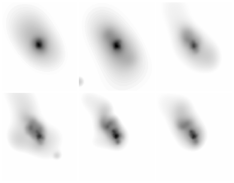
Figure 3: Six broad-band images filtered from the HETGS zeroth order image and adaptively smoothed. First row: 6-8, 3-6, 1.3-3 keV. Second row: 0.8-1.3, 0.6-0.8, 0.4-0.6 keV. Each image is $30\arcsec=2.2h_{\mathrm{75}}^{-1}$kpc on a side, 0.49″/pixel. Note the change in structure with energy. Fe K$\alpha$ emission is concentrated in the nuclear region in the 6-8 keV image. Subtle differences between the various soft X-ray bands indicate different spatial distributions for various ionization states. Starburst emission from the host galaxy disk is most apparent east of the nucleus in the 0.8-1.3 keV image.

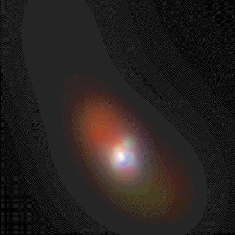
Figure 4: Three-color high energy X-ray image ($E=$1.3-3, 3-6, 6-8 keV)$=$ (r,g,b). The image is $20\arcsec=1.5h_{\mathrm{75}}^{-1}$ kpc on a side. The brightest point-like source of high-energy emission may be the inner wall of the molecular torus, reflecting X-rays from the hidden nucleus. The hard emission surrounding the hard X-ray peak may delineate reflection from the outer reaches of the obscuring torus. Extended emission to the NE and SW corresponds to the ionization cone. The SW cone is seen through and partly obscured by the disk of the host galaxy.

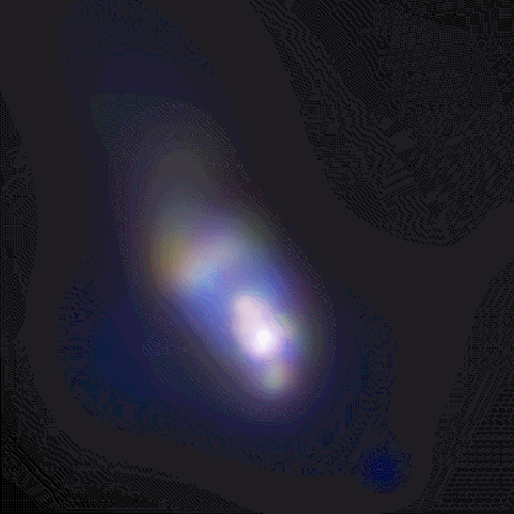
Figure 5: Three-color low energy X-ray image ($E=$0.4-0.6, 0.6-0.8, 0.8-1.3 keV)$=$(r,g,b), showing the distribution of line emission, which peaks near the nucleus. The color of the X-ray NLR ranges from blue to red, corresponding to high through lower ionization states. Same scale as Fig.  4.

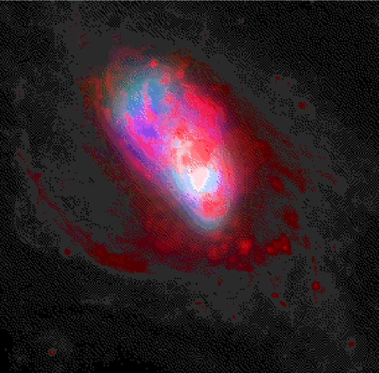
Figure 6: Composite optical H$\alpha$ (red), X-ray 0.4-0.7 keV (green), and X-ray 0.7-1.3 keV (blue) image. The H$\alpha$ image is from HST, while the lower resolution X-ray images are from Chandra. Higher ionization X-ray emission line regions are enveloped by a cocoon of lower ionization H ii filaments. Regions of strong H$\alpha$ emission in the NLR correspond to the softer X-ray emission regions in Fig.  5. H ii regions outside the photoionization cone delineate the spiral arms in the starburst disk of the host galaxy.

6 Discussion

6.1 Photoionization Model

As seen in other Seyfert 2s (Sako et al. 2000; Sambruna et al. 2001), photoionization, recombination, and photoexcitation appear to dominate the spectrum of NGC 1068. The main indicators are: (1) narrow recombination continua of N vii, O vii, and Ne ix, (2) strong forbidden lines of O vii and Ne ix (3) strong np-1s (n$>$2) lines from O vii, O viii, Ne ix, Mg xi, and Si xiii, (4) weak Fe L emission (relative to collisionally ionized plasmas). We therefore start with a pure photoionization model. In a subsequent section we assess the possibility of additional emission from a collisionally ionized component.

We model the nuclear and off-nuclear spectra of NGC 1068 using the method of Kinkhabwala et al. (2002). The geometry is a collection of clouds photoionized by an external X-ray source. Each cloud is characterized by its radial velocity, turbulent velocity, temperature, column density, and source covering fraction. The source is characterized by its 2-10 keV X-ray luminosity $L_{\mathrm{x}}$ and power-law spectral index, which we fix at $\Gamma=1.8$, a typical value for Seyferts. The velocity and turbulent velocity determine the line redshifts and widths. The electron temperature $T_{\mathrm{e}}$ controls the width of the radiative recombination continuum. The column density $N_{\mathrm{i}}$ and Doppler $b$ parameter determine the relative line contributions from recombination and photoexcitation. Note that the photoexcitation rate saturates at a larger column density for larger values of $b$. Line intensity is proportional to column density, covering fraction $f_{\mathrm{c}}$, and X-ray luminosity.

We fit the spectra to derive the flux-weighted mean cloud parameters for each ion. Spectral fitting is done with IMP, a code developed at UCSB which employs a $\chi^{2}$ minimization algorithm. For H-like and He-like ions, ($n=1-7$, l) level populations are computed by solving rate equations including terms from photoionization, recombination, and photoexcitation (Behar et al. 2001). Recombination rates for $n>7$ are extrapolated using the hydrogenic approximation. The emission line spectrum of each ion is computed from the level populations and transition rates. The radiative recombination continua (RRCs) are computed using the method of Liedahl (1999) and the photoionization cross sections of  Verner et al. (1996a). Atomic data, including energy levels, photoionization rates, recombination rates, and Einstein coefficients were calculated using the Flexible Atomic Code (FAC) 0.7.6  (Gu 2002a). Some He-like emission line wavelengths were replaced by more accurate values from  Verner et al. (1996b).

We use a more approximate treatment of Fe xvii-xxiv. Radiative recombination (RR) and dielectronic recombination (DR) line power for these ions are computed by Gu (2002b), using atomic data from FAC. Photoionization and recombination are balanced to determine relative abundances of the $i$ and $i+1$ ionic charge states. We add photoexcitation from the ground level to $n=2-5$ and include line emission from the resulting cascades. Similar to the H-like and He-like ions, the relative fluxes of photoexcitation and recombination lines depend strongly on the column density and can therefore be used to constrain it  (Sako et al. 2002).

We start our fit by fixing the Doppler $b$ parameters in the nuclear region at the values in Table  3, and fixing the emission redshift at its mean value $<z>=0.0025$. The Ne x, S xv, and Fe xvii-xxiv lines are all strongly blended. We fix their widths at $b\sim 800$ km s^-1, which appears to give a good overall model fit. Because the Fe xxv lines are strongly blended and the $n>2$ Fe xxvi lines are not detected, the column densities of these ions are not constrained and we do not include them in our fit. We fit Gaussian profiles for the the S i and Si i K$\alpha$ lines, so that they don’t skew the results for lines they are blended with. A fixed scattered continuum component ($\Gamma=1.8$) is added to the model, extrapolated from the fits of the HEG continuum (see below), so that the emission line fluxes aren’t overestimated.

Next we fit the RRC profiles to determine the electron temperature. (The width of an RRC in eV gives a rough estimate of the temperature of recombining electrons.) The O vii and Ne ix RRCs are well measured, with $T_{\mathrm{e}}=8-9\times 10^{4}$ K (Table  3). A larger range of temperatures is probably present for other ions observed that have RRCs which are too weak or blended to measure. Therefore, we fix $T_{\mathrm{e}}$ for each of these ions at a value which corresponds to an ionization parameter of peak emissivity. These temperatures were computed using the XSTAR photoionization code (Table  3). Finally, we fit for column densities and the quantity $f_{\mathrm{c}}L_{\mathrm{x}}$ for each ion (Table  4).

The fitting procedure is similar for the off-nuclear (NE cloud) spectrum. Since not all emission lines are resolved, we assume $b=800$ km s^-1, the mean value for the resolved lines. The model spectrum is convolved with a spatial profile with FWHM$=1.5\arcsec$. Because the RRCs are so weak, we can not derive accurate values for the electron temperature in the NE cloud. Again, we assume $T_{\mathrm{e}}$ values derived from XSTAR (Table  3).

6.2 Ionic Column Densities and Abundances

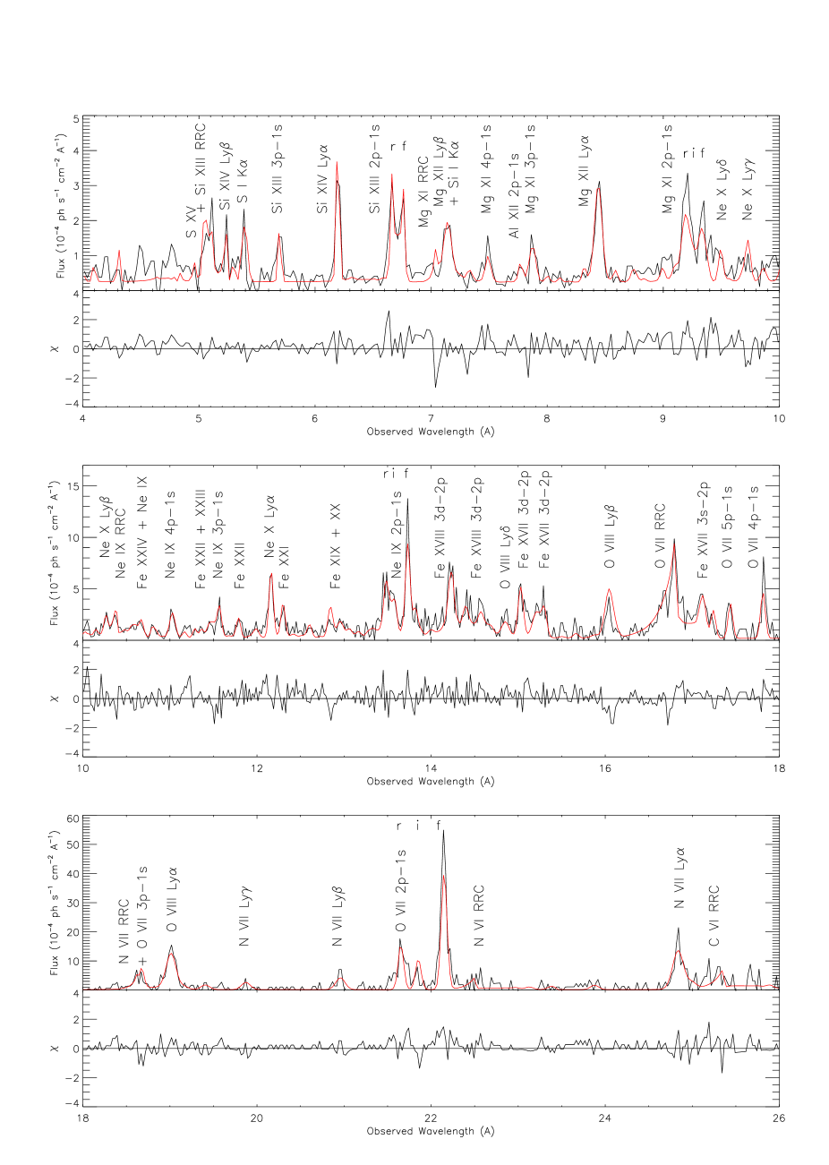
Figure 7: Photoionization model of MEG spectrum of nuclear region. Ion spectra are fit with IMP, to determine column densities and temperatures (see text). The ratios of photoexcitation to recombination lines are the primary diagnostics for column density. The widths of the RRCs are a measure of the electron temperature.

Fig.  7 shows our photoionization model fit for the nuclear region. The fit is quite good, with small residuals. Notable exceptions are the forbidden (f) line fluxes of O vii and Ne ix, which appear to be underestimated by about 20%. We conjecture that this may be due to non-Gaussian line shapes. In particular, the O vii lines appear to have underlying broad components which we do not model. The opposite problem occurs with O viii Ly$\beta$, which is overestimated because it has a narrower width than O viii Ly$\alpha$. This is difficult to understand, unless O viii Ly$\alpha$ is broadened more by scattering or there are additional emission sources which add to the line. There appears to be unmodeled excess emission in the 8.8-9.5 Å region, in the vicinity of the Mg xi triplet, which may affect our column density estimate of this ion.

We find nuclear ionic column densities (Table  4) in the range $2\times 10^{16}-6\times 10^{18}$ cm^-2, which are comparable to warm absorber column densities observed in Seyfert 1 galaxies (e.g., Kaastra et al. (2000)). We do not give formal uncertainties for the column densities, because it is hard to calculate correlated uncertainties in a $\sim 40$ parameter fit. However, we do give (90%) single-parameter uncertainties for $f_{\mathrm{c}}L_{\mathrm{x}}$. We find $<f_{\mathrm{c}}L_{\mathrm{x}}>=1.5\pm 0.2\times 10^{41}$ erg s^-1 for the nuclear region.

The large $r/f$ ($\geq 1$) values observed for Mg xi and Si xiii are nicely explained by the photoionization plus photoexcitation model. The abundances and column densities of these ions (Table  4) are relatively low so photoexcitation dominates over recombination. This is in contrast to the O vii and Ne ix ions, which have larger column densities and saturated 2p-1s resonance lines. There is therefore no need to invoke collisional excitation to explain the line ratios. We also reemphasize the fact that the strong 3p-1s, 4p-1s, and 5p-1s lines require photoexcitation, and would not be present in a collisionally excited plasma.

The column densities we derive for the nuclear region are a factor of a few higher than those derived by Kinkhabwala et al. (2002), who use a smaller radial turbulent velocity of $\sigma_{v}=200$ km s^-1 ($b=280$ km s^-1) and an additional line of sight velocity broadening of $\sigma_{v}=400$ km s^-1. It seems unlikely to us that the turbulent velocity is larger perpendicular to the axis of the ionization cone than parallel to it. However, it is possible that bulk motions of clouds may broaden the lines without affecting the resonance line optical depths in individual clouds. In that case, our measured line widths give an upper limit to $b$, and our column densities are upper limits. As pointed out by Sako et al. (2002), since the line fluxes are proportional to column density, fit column densities will be biased toward large values.

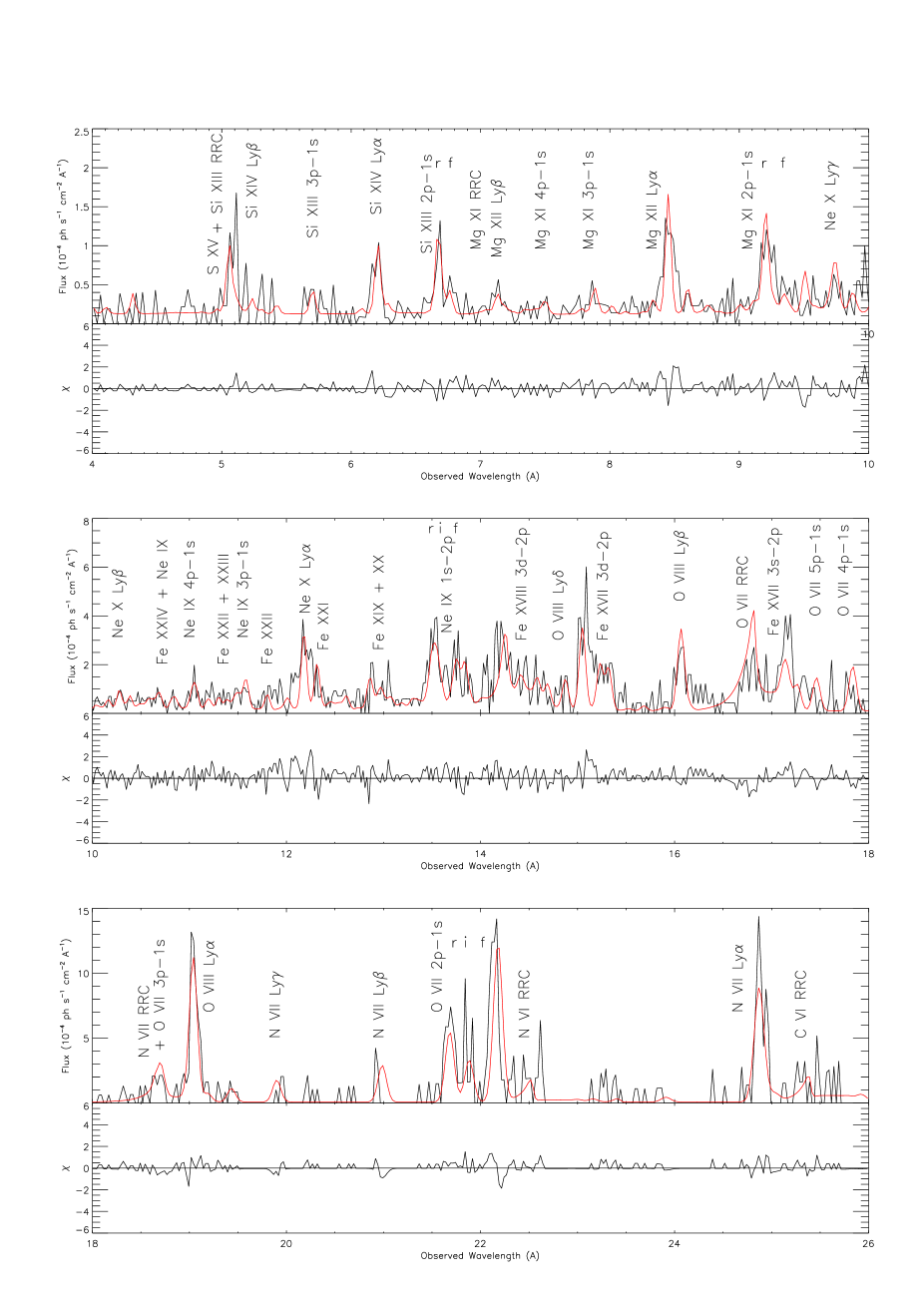
Figure 8: Photoionization model of MEG spectrum of the NE cloud. Similar to Fig.  7.

Fig.  8 shows our photoionization model fit for the NE cloud. The model does a fairly good job of representing the data, except for residuals in the 11.7-12.4 and 15-15.2 Å regions. The Fe xxi emission falls in the former band, precluding an accurate determination of the column density. The Fe xvii column density is underestimated by the model ($N_{\mathrm{i}}=4\times 10^{16}$ cm^-2). This is apparent from comparing the strengths of the 3s-2p (17.1 Å ) and 3d-2p (15.0 Å ) lines which indicate a more consistent value of $N_{\mathrm{i}}=2\times 10^{17}$ cm^-2. IMP tried to decrease the unidentified residual at 15 Å by strengthening the 3d-2p line with respect to the 3s-2p line, leading to a column density estimate which is too low. The Al xii, S xv, and Fe xxiv emission are too weak to constrain column densities. We also find an unexplained shift in the wavelength of the O vii f line, though the other lines from this series are consistent with zero redshift.

The covering fraction of the NE cloud is indistinguishable from the nuclear region, with $f_{\mathrm{c}}L_{\mathrm{x}}=9.0\pm 0.7\times 10^{40}$ erg s^-1. The small dispersion (30-50%) in $f_{\mathrm{c}}L_{\mathrm{x}}$ in both regions indicates that all ions have a similar covering fraction, assuming the source is isotropic within the ionization cone.

We estimate the equivalent hydrogen column $N_{\mathrm{H}}$ and emission measure EM$=\int n_{\mathrm{e}}^{2}dV$ for each ion (Table  4), assuming solar abundances and ion fractions modeled by XSTAR. The mean column densities averaged over all ions are $N_{\mathrm{H}}=5\pm 1\times 10^{22}$ cm^-2 in the nuclear region and $N_{\mathrm{H}}=1.4\pm 0.3\times 10^{22}$ cm^-2 in the NE cloud. The factor of 4 lower mean column density in the NE cloud accounts for the weaker forbidden lines and RRCs relative to the nuclear spectrum. Photoexcitation is relatively stronger because the resonance lines are not saturated. The relative column densities of He-like Mg and Si are even lower in the NE cloud, accounting for their very large $r/f$ ratios. Such large ratios are impossible to produce by collisional ionization in a low-density plasma. In contrast, relatively large Fe ion column densities in the NE cloud account for the strong Fe L-shell emission.

Table 4: NGC 1068 relative covering fraction, column density, and emission measure of the nuclear region (Nuc.) and NE cloud (NE). The quantity $f_{\mathrm{c}}L_{\mathrm{x}}$ is normalized to the mean for the nuclear region, $<f_{\mathrm{c}}L_{\mathrm{x}}>=1.5\times 10^{41}$. It therefore gives the relative covering fraction, assuming $L_{\mathrm{x}}$ is the same for all ions. Ionic column densities $N_{\mathrm{i}}$ are given in units of $10^{17}$ cm^-2 and equivalent hydrogen column densities in units of $10^{22}$ cm^-2. As explained in the text, IMP underestimates the column density of Fe XVII in the NE cloud. The value presented in parentheses here gives a better match to the spectrum. The emission measure EM is in units of $10^{63}$ cm^-3.

$$\begin{array}[]{p{0.13\linewidth}p{0.16\linewidth}p{0.06\linewidth}p{0.06\linewidth}p{0.07\linewidth}p{0.16\linewidth}p{0.06\linewidth}p{0.06\linewidth}p{0.07\linewidth}}\hline\cr\vskip 3.0pt plus 1.0pt minus 1.0pt\cr Ion&Nuc. $f_{\mathrm{c}}L_{\mathrm{x}}$&$N_{\mathrm{i}}$&$N_{\mathrm{H}}$&EM&NE $f_{\mathrm{c}}L_{\mathrm{x}}$&$N_{\mathrm{i}}$&$N_{\mathrm{H}}$&EM\\ \hline\cr\vskip 3.0pt plus 1.0pt minus 1.0pt\cr N {\sc vii}&0.8$\pm$0.2&49&8.3&16&0.7$\pm$0.2&27&4.6&11\\ O {\sc vii}&1.7$\pm$0.2&37&0.77&20&0.9$\pm$0.2&30&0.62&7.6\\ O {\sc viii}&0.51$\pm$0.09&59&1.3&2.1&0.40$\pm$0.07&98&2.2&1.8\\ Ne {\sc ix}&0.45$\pm$0.07&49&7.4&7.2&0.3$\pm$0.1&14&2.1&1.4\\ Ne {\sc x}&1.1$\pm$0.2&6.1&1.0&0.76&0.6$\pm$0.2&5.3&0.87&0.36\\ Mg {\sc xi}&0.39$\pm$0.07&23&12&3.9&0.8$\pm$0.3&1.2&0.61&0.62\\ Mg {\sc xii}&0.62$\pm$0.09&10&5.4&1.4&0.9$\pm$0.2&1.7&0.91&0.33\\ Al {\sc xii}&1.3$\pm$1.0&0.20&1.4&1.4&...&...&...&...\\ Si {\sc xiii}&0.8$\pm$0.1&19&11&3.6&0.8$\pm$0.3&2.3&1.3&0.42\\ Si {\sc xiv}&0.7$\pm$0.1&14&8.3&1.5&0.6$\pm$0.3&2.7&1.6&0.22\\ S {\sc xv}&0.6$\pm$0.4&20&25&3.4&...&...&...&...\\ Fe {\sc xvii}&2.5$\pm$0.6&0.44&0.30&0.72&...&(2)&...&...\\ Fe {\sc xviii}&1.5$\pm$0.4&0.81&0.66&1.0&0.4$\pm$0.1&1.5&1.2&0.51\\ Fe {\sc xix}&0.9$\pm$0.3&1.1&2.6&0.56&0.8$\pm$0.2&0.98&2.3&0.43\\ Fe {\sc xx}&0.8$\pm$0.3&1.3&1.0&0.27&0.5$\pm$0.2&0.83&0.66&0.11\\ Fe {\sc xxi}&0.7$\pm$0.3&2.3&3.2&0.15&...&...&...&...\\ Fe {\sc xxii}&1.9$\pm$0.7&0.49&0.35&0.08&0.9$\pm$0.6&0.38&0.28&0.027\\ Fe {\sc xxiii}&0.8$\pm$0.5&1.1&0.97&0.09&0.4$\pm$0.4&0.81&0.71&0.031\\ Fe {\sc xxiv}&1.0$\pm$0.9&0.62&0.89&0.05&...&...&...&...\\ \hline\cr\end{array}$$

Table 5: NGC 1068 relative elemental abundances.

$$\begin{array}[]{p{0.17\linewidth}p{0.17\linewidth}p{0.17\linewidth}p{0.17\linewidth}p{0.17\linewidth}}\hline\cr\vskip 3.0pt plus 1.0pt minus 1.0pt\cr Element&Nuclear Region&NE cloud&Solar\\ \hline\cr\vskip 3.0pt plus 1.0pt minus 1.0pt\cr N&$>0.89$&$>1.40$&0.91\\ O&1.74&6.63&6.92\\ Ne&1.00&1.00&1.00\\ Mg&0.60&0.15&0.31\\ Al&$>0.004$&...&0.024\\ Si&0.60&0.26&0.29\\ S&$>0.36$&...&0.13\\ Fe&0.15&$>0.34$&0.38\\ \hline\cr\end{array}$$

Relative elemental abundances (Table  5) are estimated by summing the ionic columns and taking the ratio with respect to neon. These are rough estimates since we are comparing clouds with a large range of ionization states, and ignore possible abundance gradients. Except for oxygen and iron, the relative abundance patterns for both the nuclear region and NE cloud are similar (within a factor of 2) to solar. Oxygen appears to be under-abundant by a factor of 4.0 in the nuclear region, but is near solar abundance in the NE cloud. Oxygen depletion by a factor of 5 was previously inferred  (Marshall et al. 1993), based on the weakness of the O viii Ly$\alpha$ line. A similar depletion by a factor of 4.0 has been inferred for nuclear molecular clouds based on a large HCN/CO intensity ratio  (Sternberg et al. 1994). The Fe abundance is depleted by a factor of 2.5 in the nuclear region, but is near solar abundance in the NE cloud.

6.3 Limits on Collisionally Ionized Plasma

Our observations confirm that line emission from the X-ray NLR in NGC 1068 is dominated by warm ($T_{\mathrm{e}}=8\times 10^{4}$) photoionized gas. However, past observations indicate that shock-heating may also be important in the NLR. The NE radio lobe terminates at a distance of $\sim 5\arcsec$ from the nucleus and has a sharp leading edge, possibly corresponding to a shock front (Wilson & Ulvestad 1987). There are also indications that the NLR clouds decelerate on the $2-4\arcsec$ scale (Crenshaw & Kraemer 2000), perhaps by plowing through the ISM of the host galaxy. Other studies have shown that photoionization by emission from shocks may be important in the optical NLR (Dopita & Sutherland 1995). In addition, pressure confinement of the NLR clouds may require the presence of a hot component with $T_{\mathrm{e}}\simeq 10^{7}$ K (Krolik et al. 1981; Ogle et al. 2000).

Adding a collisionally ionized (CI) component to the spectrum would increase the strength of the 2p-1s ($\alpha$) lines of H-like and He-like ions. The contribution to forbidden, inter-combination, and high-order Lyman lines would be relatively weaker (Kinkhabwala et al. 2002). Since the line ratios observed in NGC 1068 are closely consistent with a photoionized plasma, the 2$\sigma$ uncertainties in the $n=2-1$ line fluxes give reasonable upper limits to the contribution from CI. (Similar estimates could be made from the residual broad O vii or O viii emission.) We use the emissivities and peak temperatures of Mewe et al. (1985), who assume solar abundances. From the O vii 2p-1s line (Table  2), the 2$\sigma$ upper limit for the emission measure of a collisionally ionized component with $T=2\times 10^{6}$ K in the nuclear region is EM$<6\times 10^{62}$ cm^-3. This is 30 times smaller than the emission measure of the photoionized component (Table  4). The upper limit for a hotter collisionally ionized component with $T=1\times 10^{7}$ K is less restrictive and comparable to the emission measure of the photoionized Mg xii Ly$\alpha$ line: $EM<3\times 10^{63}$ cm^-3.

The corresponding limits on CI plasma for the NE cloud are EM$<5\times 10^{62}$ and EM$<1\times 10^{63}$ for $T=2\times 10^{6},1\times 10^{7}$, respectively. These are smaller by factors of 15 and 2.5, respectively, than the observed emission measures of photoionized O vii 2p-1s and Mg xii Ly$\alpha$. A CI component would also emit thermal bremsstrahlung continuum and strong Fe L lines (Sako et al. 2000). These are more difficult to constrain.

While we rule out collisional ionization as a major contributor to the spectrum, a weak component could be present. As we noted above, there is a region in between the nuclear region and NE cloud (Fig.  5) with a hard spectral color, similar to that in the starburst region. This region is relatively free of NLR clouds in the HST [O iii] image (Macchetto et al. 1994). With a higher S/N Chandra grating observation at the appropriate roll angle, it should be possible to get a spectrum of this region to see if it contains any hot, collisionally ionized plasma.

6.4 Characterization of the NLR Outflow

The results of the last two sections show that the X-ray NLR clouds are ionized and heated primarily by X-ray photons. The luminosity of the photoionizing source is consistent with the hidden AGN (Sect. 6.6). There is also no indication that the radio jet or lobe is a significant source of X-rays, otherwise they would appear directly in our X-ray images and spectra. Mechanical heating and ionization by shocks are apparently weak, if at all present. Any contribution to the nuclear X-ray spectrum from collisionally ionized gas, either from a starburst or shocked by the radio jet has yet to be detected.

On the other hand, there is abundant morphological and kinematic evidence that the radio jet plays a role in shaping the NLR and that it influences cloud dynamics. This leads us to believe that the radio jet interaction with the NLR is a rather gentle process and indicates a subsonic jet. An analogy may be drawn to the radio jets which evacuate bubbles in the IGM surrounding radio galaxies (e.g., Fabian et al. (2000)).

Our results also indicate that radiation power dominates over kinetic power output in NGC 1068. Kinetic power from the radio jet can at most provide a small fraction of the heating. However, radiation pressure and jet pressure may still be comparable in affecting the dynamics of the NLR. The kinematics of the NLR suggest two different regions of influence. Crenshaw & Kraemer (2000) model the inner $1.5\arcsec$ of the optical [O iii] emission line region with radially accelerating clouds in a hollow bi-cone. This structure may have naturally formed by ablation and radiative acceleration of matter from the torus. In the region of the NE cloud, the radio lobe may be expanding into the host galaxy disk (Cecil et al. 2001).

We use a grid of XSTAR 2.1  (Kallman 2001) photoionization models covering the parameter space $\log\xi=0.0-4.0$ ($\xi=L/n_{\mathrm{e}}r^{2}$) to estimate temperatures, ion fractions, and line emissivities in the X-ray NLR. We assume solar abundances. The input SED is similar to that used by Krolik & Kriss (2001). The X-ray spectrum is a power law with photon index $\Gamma=1.8$ and high energy cut-off at 100 keV. We assume that each emission line is produced in a region of peak emissivity to derive an ionization parameter and temperature for each ion.

Fig.  9a shows the distribution of $N_{\mathrm{H}}$ in the nuclear region (from Table  4) as a function of $\xi$ and $T$. There is a large amount of scatter, which we suggest is primarily due to non-solar abundances. In particular, relatively low oxygen and iron column densities suggest that these elements are under-abundant. The distribution covers a large range in ionization parameter, corresponding to a factor of 80 in density or a factor of 9 in distance from the central source.

We compute the differential emission measure (DEM) distribution (Fig.  9b) from the EM values (Table  4) assuming $\mathrm{d}(log\xi)=1.0,0.5,0.25$ for H-like, He-like, and Fe L ions, respectively. These $\mathrm{d}(log\xi)$ are estimated from the widths of the $i+1$ ion fraction curves $f_{i+1}(\xi)$ computed with XSTAR. Assuming equal-size errors for all the data points, we find a best-fit slope of -1.0 and an intercept of $log(\mathrm{d}(EM)/\mathrm{d}(\log\xi))=65.6$. The slope can be understood if we approximate the $N_{\mathrm{H}}$ distribution by $N_{\mathrm{H}}(\xi)\sim constant$. Then the emission measure drops with ionization parameter, following EM$\sim\xi^{-1}$ (Fig. 9b). Using the definitions of emission measure and ionization parameter, this also implies that the product of the mass and X-ray flux is constant,

$$M(\xi)F_{\mathrm{x}}\sim n_{e}VF_{\mathrm{x}}\sim\xi\times\mathrm{EM}=constant.$$ (1)

In other words, at any given distance from the source, there are equal masses of plasma at all observed ionization parameters. This implies a large range of density at any given location (Kinkhabwala et al. 2002). Krolik & Kriss (2001) suggest that a large range in density and temperature may result from marginal stability along the vertical branch of the cooling curve. It is also apparent from the soft X-ray image (Fig.  5) that the emission from the X-ray NLR is clumpy and azimuthally asymmetric, with a range of colors which isn’t a simple function of distance from the nucleus.

Figure 9: a) Column density and b) differential emission measure (DEM) distributions in the nuclear region. Ionization parameter $\xi$ and temperature are from XSTAR photoionization models, assuming maximum emissivity at solar abundance. The distributions cover a large range (2 decades) of ionization, with column densities of similar magnitude in each ionization state. The relatively low column densities of oxygen (X’s) and iron (squares) suggest they are under-abundant. The best fit model to the DEM distribution gives $EM\sim\xi^{-1}$, indicating equal mass at each ionization parameter.

6.5 The Torus

The obscuring region in NGC 1068 can be pictured as a collection of dusty molecular clouds surrounding the nucleus. A conical illumination pattern for the ionization cone is most simply created by a toroidal ring, but more complicated geometries may produce a similar effect. The $200\times 160$ pc (projected) central region of the Chandra image (Fig.  4) shows 3-8 keV emission from clouds surrounding the hard X-ray peak. This emission may be reflected continuum and Fe K$\alpha$ fluorescence. The lack of 1.3-3 keV line emission from this region is consistent with a low ionization parameter and high density.

The extended hard X-ray emission surrounding the nucleus coincides with the molecular CO ring measured by Schinnerer et al. (2000). The two brightest CO spots in this ring are located east and southwest of the nucleus and contain an estimated mass of $5\times 10^{6}$ $M_{\sun}$. Schinnerer et al. (2000) model the kinematics of the molecular gas with a highly warped disk. The axis of the disk is $70\degr$ to the line of sight and has a PA of $20\degr$ at a distance of $1\arcsec$ from the nucleus. A warped disk geometry can create a highly irregular X-ray illumination pattern, perhaps leading to the observed irregularity in the hard X-ray ring. Alternatively, the blobs in the ring may correspond to discrete giant molecular clouds. Much closer to the nucleus, H₂O masers outline an edge-on portion of the molecular disk with an outer radius of 30 mas (2pc) and PA$=4\degr$, and perhaps the inner surface of the torus (Gallimore et al. 1996; Greenhill et al. 1996). It is likely that the column density of the inner disk is Compton-thick, sufficient to completely obscure the direct line of sight to the nucleus. However, the molecular clouds at 100 pc scale also appear to be important in defining the geometry of the ionization cone.

A further confirmation of the obscuration model is the reflection spectrum from the nuclear region (Fig.  1). We first fit the 1.2-5 Å (2.5-10 keV) hard X-ray continuum with a PEXRAV (Magdziarz & Zdziarski 1995) component representing neutral reflection from the molecular torus. We also include Gaussian emission lines at the energies of Fe i (K$\alpha$ and K$\beta$) and Fe XXV (r and f), and account for Galactic absorption. We use the C-statistic since there are few counts per bin in the HEG spectrum. We fit a neutral reflection component with an incident power law index of $\Gamma=2.8\pm 0.2$. This unusually steep index and significant residuals in the 4-5 Å region indicate that an extra continuum component is present. Next we add a power law component from ionized reflection. The incident power law index is fixed to $\Gamma=1.8$ for both reflection components, since it is not well constrained by the data. The best fit normalizations at 1 keV for the neutral and ionized reflection components are $1.2\pm 0.2\times 10^{-2}$ ph s^-1 cm^-2 keV^-1 and $4\pm 1\times 10^{-4}$ ph s^-1 cm^-2 keV^-1, respectively. The corresponding scattered 2-10 keV luminosity from the ionized region is $\tau f_{\mathrm{c}}L_{\mathrm{x}}=4\pm 1\times 10^{40}h_{\mathrm{75}}^{-2}$ erg s^-1.

The equivalent width of the Fe i K$\alpha$ line is $1.5\pm 0.3$ keV, consistent with the value measured by BBXRT (Marshall et al. 1993). Such a large equivalent width is in agreement with Monte Carlo simulations of neutral reflection from the inner wall of a Compton-thick molecular torus  (Ghisellini et al. 1994). It is inconsistent with the smaller equivalent width of $\sim 0.5$ keV predicted for reflection from the ionized scattering region (Krolik & Kallman 1987).

6.6 Ionized Scattering Region

An ionized scattering region which gives an indirect view of the hidden nucleus is a necessary component of the Seyfert unification theory. Ultraviolet light scattered from the inner $4\arcsec$ of NGC 1068 has a wavelength-independent polarization (Antonucci et al. 1994). This is strong evidence for electron scattering as opposed to dust scattering. The optical scattering fraction is estimated at $\tau f_{\mathrm{c}}=0.015$ from spectropolarimetry of the H$\beta$ line (Miller et al. 1991). The electron-scattering region is thought to be associated with the ionized X-ray NLR  (Krolik & Kriss 1995). As shown in the last section, there is evidence for electron scattering from this region in the hard X-ray band. The scattered X-ray continuum and emission line flux from the nuclear region give estimates of $\tau f_{\mathrm{c}}L_{\mathrm{x}}$ and $f_{\mathrm{c}}L_{\mathrm{x}}$. From the ratio of these, we find an electron scattering optical depth of $\tau=0.27\pm 0.08$ (90% confidence.) Combining this result with the optical scattering fraction, the source covering fraction in the nuclear region is $f_{\mathrm{c}}\simeq 0.06$, and the luminosity of the hidden nucleus is $L_{\mathrm{x}}\simeq 2.7\times 10^{42}$ erg s^-1. The mean equivalent Thomson scattering depth associated with any given ion , $\tau=3.2\times 10^{-2}$ (derived from $<N_{\mathrm{H}}>$, Table  4), can account for 12% of the scattered X-ray continuum. Integrating over all ionization states, we can account for the total electron scattering column (Fig.  10).

The polarized broad H$\beta$ line from the central $4\arcsec$ of NGC 1068 appears to be broadened by the thermal motion of scattering electrons with mean temperature $<T_{\mathrm{e}}>=6.7\times 10^{4}$ K (Miller et al. 1991). Note that the higher value $<T_{\mathrm{e}}>=3\times 10^{5}$ K which is often quoted assumes a monochromatic incident line, whereas the lower value we quote here is for a broad incident line width estimated from the dust scattered line in the off-nuclear knot. The electron temperature we measure for the O vii ion ($T_{\mathrm{e}}=8^{+3}_{-2}\times 10^{4}$ K) is in good agreement with the value from optical spectropolarimetry. The $\sim 400$ km s^-1 redshift of the polarized broad H$\beta$ line, attributed to the outflow of the electron scattering region  (Miller et al. 1991), is consistent with the mean blue shift of the X-ray emission lines, $<v>=-410$ km s^-1.

A multi-temperature electron scattering region with $\log T(K)=4.5-6.0$ is indicated by the observed column density distribution (Fig.  9). We integrate over model temperature distributions (Fig.  10a) to predict the optical H$\beta$ profile scattered from the X-ray NLR. A simple pedestal function approximates a flat temperature distribution with a high temperature cut-off $T_{\mathrm{C}}$ and low temperature cutoff at $\log T(K)=4.5$. The area under the curve is normalized to give $\tau=0.27$. We try two different models, with $\log T_{\mathrm{C}}=5.0,5.95$. We integrate the ionic column densities over the model temperature distributions, and divide by the ionic abundances from our XSTAR models to find column density distributions (Fig.  10b) which are consistent with the observed distribution (Fig.  9).

We use a Gaussian incident BLR profile with FWHM$=2900$ km s^-1 (Miller et al. 1991) to compute the scattered H$\beta$ profile. We also include turbulent broadening of $b=1000$ km s^-1, the mean value for the X-ray emission lines (Table  3). The resulting profiles are shown in Fig.  10c, and compared to the observed polarized broad H$\beta$ line width FWHM$=4400$ km s^-1 (Miller et al. 1991). The model with $\log T_{\mathrm{C}}=5.0$ gives a better match to the observed H$\beta$ profile than $\log T_{\mathrm{C}}=5.95$. This indicates that there is relatively little plasma at hotter temperatures, or it would broaden the H$\beta$ line more than is observed. Broadening by turbulent motions in the NLR has an effect on the profile width for $\log T_{C}=5.0$, but is insignificant for $\log T_{\mathrm{C}}=5.95$ (Fig.  10c,d).

One concern is that the optical-UV bremsstrahlung from the ionized scattering region not exceed the observed continuum in that wave band. Miller et al. (1991) found that this constraint is satisfied in their models, which assume a smooth distribution of matter. However, if the scattering clouds are clumpy, then bremsstrahlung is enhanced by a factor of $<n_{\mathrm{e}}^{2}>/<n_{\mathrm{e}}>^{2}$  (Krolik & Kriss 1995). We can make a direct estimate of the optical-UV bremsstrahlung by integrating over the DEM$(T)$ curve (Fig.  9b). We predict peak emission of $\nu F_{\nu}=8.4\times 10^{-14}$ erg s^-1 cm^-2 at $\lambda=3000$ Å. This is 40 times lower than the Miller et al. (1991) estimate of $\nu F_{\nu}<3.4\times 10^{-12}$ erg s^-1 cm^-2 (970Å), which assumed a radial density distribution of $n_{\mathrm{e}}\sim r^{-2}$. Hence bremsstrahlung emission is much weaker than the scattered optical-UV light and will be very difficult to detect.

Our Chandra observations confirm the hypothesis that the X-ray NLR and the optical/X-ray electron scattering region are one and the same. Both occupy the same extended region in the central $3\arcsec$ of the galactic nucleus, and have roughly the same optical depth and electron temperature. The expected variability timescale is the light-crossing time, which is 240 years. This is apparently at odds with a recent report of 20% variability in 4 months of the scattered X-ray continuum and 60% variability of the Fe xxv (6.7 keV) emission line flux  (Colbert et al. 2002). However, we can not rule out the possibility that the continuum variability comes from a point source which contributes a significant fraction of the flux. There are not enough photons in our Chandra observation to obtain separate images of the Compton-reflected and electron-scattered components of the X-ray continuum. Similarly, we can not spatially distinguish the regions of Fe i and Fe xxv K$\alpha$ emission. It will be important to follow up with additional high-resolution Chandra spectroscopy to see if the Fe xxv line variability is confirmed.

Figure 10: a) Model temperature distributions of optical depth in the nuclear scattering region, assuming two different cut-off temperatures ($\log T_{\mathrm{C}}(K)=$5.0,5.95; dash and dot-dash). b) Corresponding column density distributions, both consistent with the observed distribution in Fig. 9. c) Scattered H$\beta$ profiles, integrated over the two model temperature distributions in panel a. The observed (incident and scattered) line profiles are the solid curves (Miller et al. 1991). The dashed and and dot-dashed curves show the predicted scattered profiles, including both thermal and turbulent broadening (1000 km s^-1). d) Similar to c), without turbulent broadening.

7 Conclusions

Chandra HETGS X-ray spectroscopy and imaging of NGC 1068 provide new diagnostics of the spatially resolved narrow-line region and support the Seyfert unification model. The X-ray spectrum contains emission lines from a large range of ions in the NLR, and fluorescence from the molecular torus. The X-ray emitting plasma in the extended NLR is primarily photoionized and there is no evidence for a collisionally ionized component. Our previous claim of such a component in NGC 4151 (Ogle et al. 2000) was confused by the effects of photoexcitation.

Observations of the narrow Fe K$\alpha$ line show that it is produced predominately in the nuclear region, near the location of the hidden nucleus. Its equivalent width is consistent with obscuring torus models. It also appears that we have detected and resolved the outer regions of the molecular torus in hard X-rays. The hard X-ray continuum spectrum from the nuclear region consists of a Compton hump from neutral scattering and an electron scattered component.

We derive ionic column densities, equivalent hydrogen column densities, and emission measure distributions for both the nuclear region and a cloud $3\arcsec$ NE of the nucleus. The column density of the X-ray NLR can account for the entire electron scattering column in the nuclear region. In addition, its temperature and velocity are sufficient to cause the observed broadening and redshift of the scattered optical broad lines. These facts are all consistent with electron scattering in the X-ray NLR providing the view of the hidden Seyfert 1 nucleus.

The results for the X-ray NLR in NGC 1068 may also have important implications for the properties of ionized (warm) absorbers seen in the spectra of many Seyfert 1 galaxies. Similar velocities and ionization parameters are found in warm absorbers and the X-ray NLR. We see from Chandra observations of NGC 1068 that AGN outflows can be clumpy and show a wide range of ionization $\log\xi=1.0-3.0$. The differential emission measure distribution indicates roughly equal mass in each ionization state in this range. The emission seen in various UV and X-ray lines, though occupying roughly the same region, must come from clouds of greatly different ionization, temperature, and density. It is important to understand the equilibrium among the different phases to develop a complete picture of AGN outflows.