COBE-DMR constraints on the nonlinear coupling parameter: a wavelet based method

Abstract

Nonlinearity introduced in slow-roll inflation will produce weakly non-Gaussian CMB temperature fluctuations. We have simulated non-Gaussian large scale CMB maps (including COBE-DMR constraints) introducing an additional quadratic term in the gravitational potential.The amount of nonlinearity being controlled by the so called nonlinear coupling parameter $f_{nl}$. An analysis based on the Spherical Mexican Hat wavelet was applied to these and to the COBE-DMR maps. Skewness values obtained at several scales were combined into a Fisher discriminant. Comparison of the Fisher discriminant distributions obtained for different nonlinear coupling parameters with the COBE-DMR values, sets a constraint of $|f_{nl}|<1100$ at the $68\%$ confidence level. This new constraint being tighter than the one previously obtained by using the bispectrum by Komatsu et al. (2002).

1 Introduction

The COBE-DMR data have been found to be compatible with Gaussianity by several methods based on real (Torres et al. 1995; Kogut et al 1996; Schmalzing & Górski 1997; Novikov et al. 2000), spherical harmonic (Banday et al. 2000; Sandvik & Magueijo 2000; Komatsu et al. 2002) and wavelet space (Mukherjee, Hobson & Lasenby 2000; Aghanim, Forni & Bouchet 2000; Barreiro et al. 2000; Cayón et al. 2001). CMB observations by Boomerang, DASI and MAXIMA-I (Netterfield et al. 2001; Pryke et al. 2001; Stompor et al. 2001) seem to indicate that any possible non-Gaussianity present in the data will more likely be produced by non-standard Inflationary models.

It is important at the moment to study the characteristics of the non-Gaussianity introduced by the alternative theories to standard Inflation. One of the simplest alternative scenarios that will generate weakly non-Gaussian CMB fluctuations is one based on slow-roll inflation. Investigated by Salopek & Bond (1990) and Gangui et al. (1994), this model generates non-Gaussianity in matter and radiation fluctuation fields through features appearing in the inflaton potential. In the CMB context, the model has been studied by Komatsu & Spergel (2001), Verde et al. (2001) and Komatsu et al. (2002). The gravitational potential includes now a quadratic term whith an amplitude regulated by the so called non-linear coupling parameter (see Section 2). Verde et al. (2001) conclude in their paper that CMB data will be more sensitive to the non-Gaussianity generated by these models than observations of high redshift objects. A semianalytical expression of the bispectrum generated by this model is presented in Komatsu & Spergel (2001). The minimum non-linear coupling parameter values that will produce detectable non-Gaussianity (based on the bispectrum and skewness statitics) in different CMB data sets are estimated. These values are however larger than the ones expected from slow-roll inflation theories. Komatsu et al. (2002) revised the constraint impossed by COBE-DMR data on the non-linear coupling parameter based on the normalized bispectrum. This constraint (slightly larger than the one estimated by Komatsu & Spergel 2001), though very weak to say much about slow-roll inflation is in any case interesting in itself. Deviations from slow-roll inflation might include larger values of the non-linear coupling parameter generating non-Gaussianities that could be detected by CMB experiments.

We want to asses in this paper which is the minimum value of the non-linear coupling parameter that would be constraint by the COBE-DMR data based on a wavelet space statistic. Comparison of this constraint with the one obtained using the normalized bispectrum is an important comparison between two methods that will potentially be used in the analysis of future CMB data. At the moment, simulations of CMB temperature fluctuations generated by the slow-roll inflation model here considered are possible at large angular scales. The outline of the paper is the following. The simulations used in this work are described in Section 2. The method used to constrain the non-linear coupling parameter is based on the Fisher discriminant built on skewness values corresponding to wavelet coefficient maps at several scales. These method is presented in Section 3. Results are summarized in Section 4. Section 5 is dedicated to discussion and conclusions.

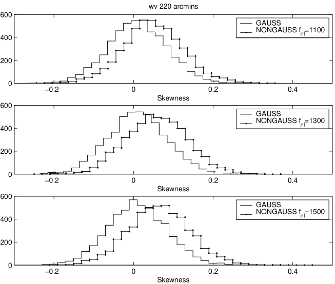
Figure 1: Distribution of skewness values obtained from simulated Gaussian (solid line) and NonGaussian (solid-dotted line) maps after convolution with a Spherical Mexican Hat wavelet of size 220 arcmins. Three different NonGaussian cases are presented with $f_{nl}=1100,1300,1500$ from top to bottom respectively

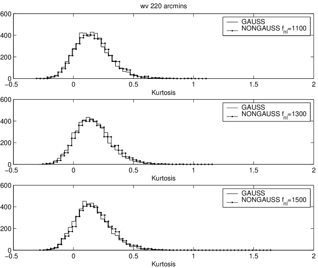
Figure 2: Distribution of kurtosis values obtained from simulated Gaussian (solid line) and NonGaussian (solid-dotted line) maps after convolution with a Spherical Mexican Hat wavelet of size 220 arcmins. Three different NonGaussian cases are presented with $f_{nl}=1100,1300,1500$ from top to bottom respectively

2 Simulations

At large scales, the CMB temperature fluctuations are dominated by the Sachs-Wolfe effect and are therefore proportional to the fluctuations of the gravitational potential. Weakly non-Gaussian CMB temperature fluctuations will be generated by the introduction of a nonlinear term in the gravitational potential $\phi(\vec{n})$

$$\phi(\vec{n})=\phi_{L}(\vec{n})+f_{nl}(\phi_{L}^{2}(\vec{n})-<\phi^{2}(\vec{n})>),$$

where $\phi_{L}$ refers to the linear part of the gravitational potential, $f_{nl}$ is the nonlinear coupling parameter controlling the amount of non-Gaussianity introduced and the brackets indicate a volume average. The linear part of the gravitational potential gives rise to CMB temperature fluctuations characterised by a power spectrum that in our case is assumed to be a CDM power spectrum (computed with the CMBFAST software) with $\Omega_{b}=0.05,\Omega_{c}=0.3,\Omega_{v}=0.65,\Omega_{\nu}=0,H_{o}=65$ km/s/Mpc and $n=1$ and normalized to $Q_{rms}=18\mu k$.

We generate Gaussian as well as non-Gaussian (as explained above) HEALPix (Górski, Hivon & Wandelt 1999) projected CMB maps that include the observational constraints affecting the COBE-DMR maps. We apply the method to the 4-year 53 and 90 GHz COBE-DMR maps after adding them using inverse-noise-variance weights. These maps have a resolution of $N_{side}=32$ corresponding to a pixel size of $\approx 110^{\prime}$. Only the pixels outside the extended Galactic cut – described in Banday et al (1997) but explicitly recomputed for the HEALPix sky maps – are considered in the computation. Best-fit monopole and dipole are removed from the pixels under analysis. To follow these COBE-DMR observational constraints, the simulated Gaussian and non-Gaussian maps are convolved with a window function characterising the COBE-DMR one as defined in Wright et al. (1994). Noise maps, generated with the same observation pattern and rms noise levels as the COBE-DMR data, are added to them. The extended Galactic cut is also impossed to these simulated maps and a best-fit monopole and dipole is as well removed from the pixels outside the cut. 5000 simulated maps are used in the statistical comparison described in the next section.

3 Method

The aim of this work is to obtain the constraint impossed by the COBE-DMR data on the nonlinear coupling parameter $f_{nl}$. We use an approach based on the information provided by wavelets at several scales. There are at the moment only two wavelets implemented on the sphere that have been used in CMB analyses; the Spherical Mexican Hat wavelet (Cayón et al. 2001; Martínez-González et al. 2001) and the Spherical Haar wavelet (Tenorio et al. 1999; Barreiro et al. 2000). The former has proved to be more efficient than the Spherical Haar wavelet in detecting certain kind of non-Gaussianity as shown in Martínez-González et al. (2001). Moreover, the non-Gaussianity introduced in the CMB maps by the nonlinear term added to the gravitational potential, is not expected to be dominated by any prefered direction. Therefore a wavelet with spherical symmetry, as the Spherical Mexican Hat, appears to be more appropriate to analyse these data.

Simulated Gaussian and non-Gaussian maps as well as the original COBE-DMR maps are convolved with Spherical Mexican Hat wavelets with sizes ranging from 2 (220 arcmins) to 8 pixels. For these maps we compute skewness and kurtosis. The non-Gaussianity introduced by the nonlinear term added to the gravitational potential will be visible when we compare distributions for these statistics for the Gaussian and non-Gaussian cases. Moreover, since the nonlinear term is small in amplitude and quadratic, we will expect the third order cumulant to be larger than any of the higher order cumulants. As an example, the skewness and kurtosis distributions of Gaussian and non-Gaussian maps at 220 arcmins are compared in Figures 1 and 2. The weakly non-Gaussianity introduced in the CMB simulations reflects in skewed distributions. As expected, the kurtosis seems not to be affected by the nonlinear term. We will therefore only use the skewness in our final analysis.

In order to combine all the information we have at the seven scales used in the analyses we use the Fisher discriminant. Being $\vec{x}$ the 7-dimensional data vector including the skewness values at the seven scales, the Fisher discriminant $t(\vec{x})$ is defined as

$$t(\vec{x})=(\vec{\mu}_{o}-\vec{\mu}_{1})^{T}W^{-1}\vec{x}.$$

Where the $o$ subscript refers to the Gaussian case and the $1$ subscript refers to the non-Gaussian cases. $W=V_{o}+V_{1}$ gives the sum of the covariance matrixes and $\vec{\mu}_{o},\vec{\mu}_{1}$ refer to the mean values obtained for the Gaussian and non-Gaussian case respectively. This statistic has been previously used in other analysis related to detecting non-Gaussianity in the CMB (Barreiro & Hobson 2001; Martínez-González et al. 2001). We establish the COBE-DMR constraint on $f_{nl}$ by comparing the COBE-DMR Fisher discriminant value with the Fisher discriminant distributions obtained for non-Gaussian simulations.

4 Results

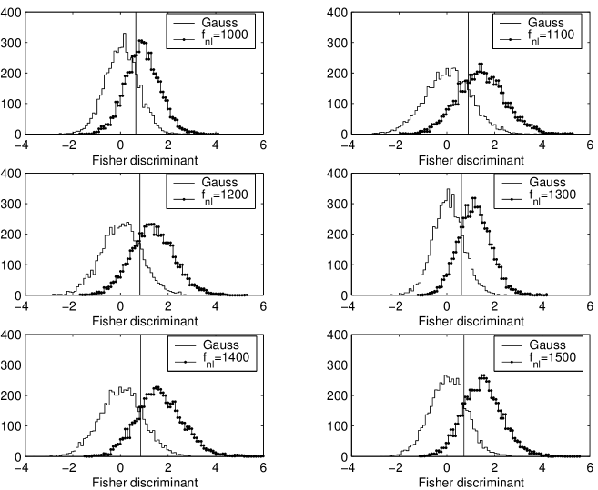
Figure 3: Distribution of Fisher discriminant values obtained from simulated Gaussian (solid line) and NonGaussian (solid-dotted line). The non-Gaussian simulations are generated with nonlinear coupling coefficients $f_{nl}=1000,1100,1200,1300,1400,1500$. Vertical bars indicate the locus of the COBE-DMR Fisher discriminant for each case.

Fisher discriminant distributions are presented in Figure 3 for several non-Gaussian cases characterised by the value of the nonlinear coupling coefficient. Comparison of Figures 1 and 3 shows the expected Fisher discriminant result of increasing the power to distinguish two distributions. Vertical bars in Figure 3 are drawn at the COBE-DMR Fisher discriminant values for each non-Gaussian case considered. In order to obtain a constraint on $f_{nl}$ we calculate the probability of observing a Fisher discriminant value larger than the COBE-DMR one for each of the non-Gaussian cases. These probabilities are presented in Table 1. As one can see the COBE-DMR data set a constraint on $f_{nl}<1100$ at the $68\%$ confidence level.

Table 1: Probability of having non-Gaussian values of the Fisher discriminant larger(for the positive $f_{nl}$ values) or smaller (for the negative $f_{nl}$ values) than the COBE-DMR values

$f_{nl}$	Prob($\%$)
1000	63.0
1100	68.7
-1100	98.9
1200	70.2
1300	76.6
-1300	99.4
1400	78.6
1500	81.2
2000	93.4
2500	97.9
3000	99.3

In all previous calculations we have only considered positive values of the nonlinear coupling coefficient. To study the effect of having a negative $f_{nl}$ on the Fisher discriminant values, we have simulated 5000 non-Gaussian maps with $f_{nl}=-1100,-1300$. The distribution of temperature fluctuations in the map would be expected in this case to be shifted towards negative values in the same way as the distribution of temperature fluctuations is shifted towards positive values for $f_{nl}>0$ (as can be seen from the skewness distributions presented in Figure 1). Therefore, we would expect the distribution of skewness values in the case of $f_{nl}<0$ to be towards the left of the distribution for $f_{nl}=0$. Same behaviour is observed for the Fisher discriminant distributions as can be seen in Figure 4. The cases for $f_{nl}=1100,1300$ are also included in that figure for comparison. The power to distinguish the Gaussian and non-Gaussian distributions is approximately the same for the positive and negative values of $f_{nl}$. At the $95\%$ confidence level, the power of the Fisher discriminant test is $40.7\%,39.1\%,51.5\%,48.6\%$ for $f_{nl}=1100,-1100,1300,-1300$ respectively. The same “symmetric” behaviour would therefore be expected for the any negative $f_{nl}$ value in relation to the positive one. As one can see from Figure 4 the locus of the COBE-DMR Fisher discriminant value does not change much (the probability of obtaining Gaussian values larger than the COBE-DMR ones is approximately the same). The probability of having non-Gaussian values smaller than COBE-DMR ones is $98.9\%$ for the case of $f_{nl}=-1100$ and $99.4\%$ for the case of $f_{nl}=-1300$. The negative values of $f_{nl}$ are therefore better constrained than the positive ones. We can conclude that the COBE-DMR data set a constraint on the absolute value of the nonlinear coupling parameter of $|f_{nl}|<1100$ at the $68\%$ confidence level.

In order to account for the possible influence of foregrounds we have also analysed the COBE-DMR data after foreground removal (using COBE-DIRBE data). The results obtained are consistent with the ones presented above.

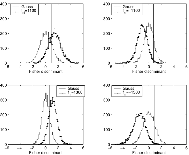
Figure 4: Distribution of Fisher discriminant values obtained from simulated Gaussian (solid line) and NonGaussian (solid-dotted line). The non-Gaussian simulations are generated with nonlinear coupling coefficients $f_{nl}=1100,-1100,1300,-1300$. Vertical bars indicate the locus of the COBE-DMR Fisher discriminant for each case.

5 Discussion and Conclusions

Weakly non-Gaussian CMB temperature fluctuations can be generated by the presence of a nonlinear term in the gravitational potential. The amount of nonlinearity can be controlled by the so called nonlinear coupling parameter $f_{nl}$. At large scales, the CMB temperature fluctuations are proportional to the gravitational potential. Simulations of weakly non-Gaussian CMB temperature fluctuations maps at these large scales are therefore reasonably easy to make.

The aim of this paper is to set a constraint on the value of the nonlinear coupling parameter by using the COBE-DMR data. We perform 5000 simulations of Gaussian and several non-Gaussian models characterised by the value of $f_{nl}$, impossing the COBE-DMR observational constraints. With the aid of the Spherical Mexican Hat wavelet, we are able to obtain the skewness of these maps at several scales. All this information is combined into the Fisher discriminant. Distributions of this statistic are used to set the constraint on $f_{nl}$ by comparing the ones obtained from the non-Gaussian simulations to the COBE-DMR values. With this method we are able to set $|f_{nl}|<1100$ at the $68\%$ confidence level. This is a tighter contraint than the one previously found by Komatsu et al. (2002). They obtain the best-fit value of $f_{nl}$, by fitting the observed COBE-DMR bispectrum to a theoretical non-Gaussian model. They estimate statistical uncertainties of this parameter and place a $68\%$ confidence limit on $f_{nl}$ as $|f_{nl}|<1500$ for the extended cut.

A method based on wavelets in which an efficient combination of information from different scales is used, has been shown to be very powerful in order to test the non-Gaussianity introduced in CMB maps by a nonlinear term in the gravitational potential. This work has been carried out at large scales at which the Sachs-Wolfe effect dominates. However tighter constraints are expected to be obtained from the analysis of higher resolution maps.

References

- [1] Aghanim, N., Forni, O. & Bouchet, F.R. 2000, astro-ph/0009463
- [2] Banday, A.J., Górski, K.M., Bennett, C.L., Hinshaw, G., Kogut, A., Lineweaver, C.H., Smoot, G.F. & Tenorio, L. 1997, ApJ, 475, 393
- [3] Banday, A.J., Zaroubi, S. & Górski, K.M. 2000, ApJ, 533, 575
- [4] Barreiro, R.B. & Hobson, M.P. 2001, MNRAS, 327, 813
- [5] Barreiro, R.B., Hobson, M.P., Lasenby, A.N., Banday, A.J., Górski, K.M. & Hinshaw, G. 2000, MNRAS, 318, 475
- [6] Cayón, L., Sanz, J.L., Martínez-González, L., Banday, A.J., Argüeso, F., Gallegos, J.E., Górski, K.M. & Hinshaw, G. 2001, MNRAS, 326, 1243
- [7] Gangui, A., Lucchin, F., Matarrese, S. & Mollerach, S. 1994, ApJ, 430, 447
- [8] Górski, K.M., Hivon, E. & Wandelt, B.D. (astro-ph/9812350) 1999, Proceedings of the MPA/ESO Conference on Evolution of Large-Scale Structure: from Recombination to Garching, 2-7 August 1998; eds. A.J. Banday, R.K. Sheth and L. Da Costa, PrintPartners IPSKAMP NL (1999)
- [9] Kogut, A., Banday, A.J., Bennett, C.L., Górski, K., Hinshaw, G., Smoot, G.F. & Wright, E.L. 1996, ApJ, 464, L29
- [10] Komatsu, E., Wandelt, B.D., Spergel, D.N., Banday, A.J. & Gorski, K.M. 2002, ApJ, 566, 19
- [11] Martínez-González, E., Gallegos, J.E., Argüeso, F., Cayón, L. & Sanz, J.L. 2001, astro-ph/0111284
- [12] Mukherjee, P., Hobson, M.P. & Lasenby, A.N. 2000, MNRAS, 318, 1157
- [13] Netterfield, C.B. et al. 2001, astro-ph/0104460
- [14] Novikov, D., Schmalzing, J. & Mukhanov, V.F. 2000, A&A 364, 17
- [15] Pryke, C. et al. 2002, ApJ, 568, 46
- [16] Salopek, D.S. & Bond, J.R. 1990, Phys. Rev.D. 42, 3936
- [17] Sandvik, H.B. & Magueijo, J. 2000, astro-ph/0010395
- [18] Schmalzing, J. & Górski, K.M. 1997, MNRAS, 297, 355
- [19] Stompor, R. et al. 2001, ApJ, 561, L7
- [20] Tenorio, L., Jaffe, A.H., Hanany, S. & Lineweaver, C.H. 1999, MNRAS, 310, 823
- [21] Torres, S., Cayón, L., Martínez-González, E. & Sanz, J.L. 1995, MNRAS, 274, 853
- [22] Verde, L., Jímenez, R., Kamionkowski, M. & Matarrese, S. 2001, MNRAS, 412
- [23] Wright, E.L., Smoot, G.F., Kogut, A., Hinshaw, G., Tenorio, L., Lineweaver, C.H., Bennett, C.L. & Lubin, P.M. 1994, ApJ, 420, 1