The number and metallicities of the most metal-poor stars

Abstract

Simple, one-zone models for inhomogeneous chemical evolution of the Galactic halo are used to predict the number fraction of zero-metallicity, Population III stars, which currently is empirically estimated at $<4\times 10^{-4}$. These analytic models minimize the number of free parameters, highlighting the most fundamental constraints on halo evolution. There are disagreements of at least an order of magnitude between observations and predictions in limiting cases for both homogeneous Simple Model and Simple Inhomogeneous Model (SIM). Hence, this demonstrates a quantitative, unambiguous discrepancy in the observed and expected fraction of Population III stars. We explore how the metallicity distribution of the parent enrichment events $f(z_{0})$ drives the SIM and predictions for the Population III fraction. The SIM shows that the previously-identified “high halo” and “low halo” populations are consistent with a continuous evolutionary progression, and therefore may not necessarily be physically distinct populations. Possible evolutionary scenarios for halo evolution are discussed within the SIM’s simplistic one-zone paradigm.

The values of $z_{0}$ depend strongly on metal dispersal processes, thus we investigate interstellar mixing and mass transport, for the first time explicitly incorporating this into a semi-analytic chemical evolution model. Diffusion is found to be inefficient for all phases, including the hot phase, of the interstellar medium (ISM): relevant diffusion lengths are 2 – 4 orders of magnitude smaller than corresponding length scales for turbulent mixing. Rough relations for dispersal processes are given for multiphase ISM. These suggest that the expected low-metallicity threshold above zero is consistent with the currently observed limit.

1 Introduction

The search for zero-metallicity, Population III stars provides one of the most fundamental empirical constraints on the assembly of galaxies and the process of chemical evolution. In spite of decades of methodical searches, to date no bona fide Population III stars, i.e., having zero metallicity, have been identified (e.g., Beers 1999). This lack is often cited as problematic (e.g., Bond 1981; Cayrel 1996; Larson 1998): a first generation of stars must have existed, and to date, the stellar initial mass function (IMF) empirically has appeared rather robustly universal. We would therefore naively expect some surviving Population III stars today. Yet, the on-going efforts of Beers et al. (e.g., 1992; 1999) show a current upper limit to the fraction of Population III stars in the Galactic halo of $<4\times 10^{-4}$ (see §1.1 below). However, there is surprisingly little quantitative discussion on the expected relative fraction $F_{\rm III}$ of Population III stars. Bond (1981) first emphasized the existence of a discrepancy in the observed fraction of low-metallicity stars for the Galactic halo population, in terms of the Simple Model for galactic chemical evolution. A few additional estimates for $F_{\rm III}$ have been made, and these vary by orders of magnitude, ranging from $F_{\rm III}\lse 10^{-1}$ (Bond 1981) to $10^{-4}$ (Tsujimoto et al. 1999). A primary objective of this paper is to further discuss the parameters that determine $F_{\rm III}$ and make better-understood predictions.

Meanwhile, these searches for the most metal-poor stars in the Galaxy have more clearly determined their metallicity distribution. At present, the lowest-metallicity stars identified thus far have logarithmic abundance relative to solar of [Fe/H] $\sim-4$. There has been a parallel effort obtaining abundance measurements of the lowest-metallicity Lyman $\alpha$ absorption-line systems (e.g., Lu et al. 1996; Songaila & Cowie 1996). These are currently in the range of [Fe/H] $\sim-3$ (Lu et al. 1996; Prochaska & Wolfe 2000; Ellison et al. 2000). Pettini (2000) emphasizes that metals have been detected in all Ly $\alpha$ forest systems that have been searched to date, including those with the lowest column densities (Ellison et al. 2000; Songaila & Cowie 1996). It therefore has been suggested that [Fe/H] in the range $-3$ to $-4$ represents a physical minimum threshold in metallicity. Indeed, it is widely thought that the abundances of Galactic halo stars in this range exhibit the yields of only a few, even individual, supernovae (e.g., Audouze & Silk 1995; Ryan et al. 1996; Shigeyama & Tsujimoto 1998).

How many Population III stars can we expect to find today? Besides these, is there indeed a minimum metallicity threshold? If so, is its value of order [Fe/H] $\sim-4$? Predictions for these parameters will necessarily have large uncertainties, since they depend on poorly constrained relations between cosmic galaxy evolution, star formation, and multiphase interstellar medium. Nevertheless, some insight on these fundamental problems is possible from simple arguments based on first principles and dominant effects. These are re-examined here, with special emphasis on interstellar element dispersal, and lead to new estimates of the expected numbers of Population III stars and the low-metallicity threshold. The results also offer insight on the star formation processes in the early Universe.

1.1 Current empirical limit

We first estimate the current limit on $F_{\rm III}$ for the Galactic halo. Beers (1999) reports that his group’s survey of metal-poor stars in the solar neighborhood (e.g., Beers et al. 1992; hereafter BPS) to date finds at least 373 stars with [Fe/H] $<-2.5$. However, none have been found at zero metallicity, or even at [Fe/H] $\lse-4$. Their survey is not designed as a complete survey of the halo metallicity distribution function (MDF), thus we compare with the halo MDF measured by Carney et al. (1996), who find 16% of halo stars to have [$m$/H] $<-2.5$. Their measurements of [$m$/H], a logarithmic metal abundance relative to solar, are calibrated to correspond closely with [Fe/H] (Carney et al. 1987). Thus, assuming that all the BPS stars with [Fe/H] $<-2.5$ are halo members, we find that the metal-poor tail examined by the BPS survey implies a fraction of zero-metallicity stars $F_{\rm III}<4\times 10^{-4}$.

2 Predictions in the homogeneous limit

What value of $F_{\rm III}$ should we expect? The very simplest generalization is that, for a present-day mean metallicity $\bar{z}_{1}$, the number of generations of enrichment events is:

$$n=\bar{z}_{1}/\bar{z}_{0}\quad,$$ (1)

where $\bar{z}_{0}$ is the mean metallicity of these individual enrichment events. The present-day fraction of Population III stars is therefore $F_{\rm III}\sim 1/n$. Thus, if we wish to interpret the metal-poor empirical thresholds as estimates of $\bar{z}_{0}$, we can set a lower limit on $F_{\rm III}$. Taking $\bar{z}_{0}\sim 10^{-5}\ \rm\,Z_{\odot}$ therefore implies $n\sim 10^{5}$ to attain solar metallicity. Likewise, the Galactic halo, having a mean metallicity around $0.1\rm\,Z_{\odot}$, requires $n\sim 10^{4}$, and hence $F_{\rm III}\sim 10^{-4}$.

However, this overly simplistic analysis does not account for the consumption of gas to form stars, assuming a closed system. We therefore turn next to the Simple Model for homogeneous chemical evolution (e.g., Schmidt 1963; Pagel & Patchett 1975; Tinsley 1980) to describe the relationship between $n$ and metallicity $z$. The effect of gas consumption naturally implies larger numbers of stars for earlier generations, thereby increasing the predicted $F_{\rm III}$.

As Bond (1981) demonstrated, the Simple Model predicts a final metallicity distribution:

$$\phi(z)=y^{-1}\ \exp(-z/y)\quad.$$ (2)

For yield $y\simeq z_{1}\simeq 0.02$, this implies that about 15% of Galactic halo stars should have [Fe/H] $\leq-2.5$. At the time of Bond’s work, none of 129 halo objects, namely stars from the Carney et al. (1979) proper-motion survey and halo globular clusters, had been found to have [Fe/H] $<-2.6$. Ten years later, Ryan & Norris (1991) reported that, within the errors, their newer dataset did show agreement between the prediction and observations; and another five years later, Carney et al. (1996) report 16% of stars in their expanded survey have [Fe/H] $<-2.5$, a value in remarkable agreement with the prediction of equation 2!

Is Bond’s discrepancy resolved? Let us now consider the number of stars expected below the current observational limit of [Fe/H] $<-4$. Equation 2 predicts a fraction $5\times 10^{-3}$ of halo stars to have metallicities below this value. This is about an order of magnitude greater than the observed limit found above: about 12 stars should have been found by the BPS survey, with assumptions in §1.1. Thus it appears that Bond’s discrepancy has simply shifted to lower metallicity. While our search techniques are greatly improved, the saga of Bond’s original discrepancy is an important caveat against prematurely concluding that the discrepancy exists.

Therefore, the limit on observed zero-metallicity, i.e., Population III, stars themselves offers perhaps a more powerful constraint on the early chemical evolution and star formation conditions. However, it is difficult to use the Simple Model to robustly predict the actual fraction of zero-metallicity stars: equation 2 shows that for low metallicities, the predicted number of stars per unit $z$ is roughly constant. Because complete homogeneity is assumed, the Simple Model cannot accommodate the stochastic effects that dominate the first generations of contamination. We therefore require an inhomogeneous model for chemical evolution that can account for the quantization and stochastic nature of the earliest enrichment events.

3 Inhomogeneous limit: no mixing

As mentioned above, the element abundances of the most metal-poor stars are generally interpreted as reflecting the yields of the first generations of stars. The impetus is particularly provided by (McWilliam et al. 1995): the marked change in abundance patterns for [Fe/H]$<-2.4$, as is expected when these properties are determined stochastically rather than statistically; and the large dispersions in these properties, that are qualitatively consistent with stochastic supernova (SN) yields. As emphasized by McWilliam et al. (1995) and Ryan et al. (1996), these abundance dispersions now force us to abandon the Simple Model and consider inhomogeneous chemical evolution for the lowest-metallicity populations.

In the limit of no ISM mixing, inhomogeneous chemical evolution can be described in the simplest case as overlapping regions of contamination. Oey (2000; hereafter Paper I) presents such a model. This model is essentially an inhomogeneous variation of the Simple Model, and offers an opposing limit for the case of no homogenization. We will refer to this as the Simple Inhomogeneous Model (SIM), and briefly review some of the basics here. We note that Argast et al. (2000) present a similar model that is numerically calculated; their study differs in that they consider only individual SNRs, while Paper I considers contamination from multi-SN superbubbles. In addition, the analytic development in Paper I more clearly shows the relevant parameterizations that also apply to the numerical results.

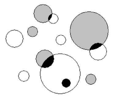
Figure 1: Schematic illustration of the Simple Inhomogeneous Model described by Oey (2000), for $n=2$. Each generation $k$ randomly occupies filling factor $Q$. Here, $k=1$ is shown by white regions and $k=2$ by gray regions. Overlapping regions for $j=2$ are shown in black, while $j=1$ corresponds to both white and gray regions.

For the metallicity distribution function of long-lived stars:

$$N(z)=\frac{1}{n}\ \sum_{j=1}^{n}\ \sum_{k=j}^{n}\ D_{k-1}\ P_{j,k}\ N_{j}(z)\quad,$$ (3)

where $N_{j}(z)$ is the MDF for stars born in areas resulting from $j$ overlapping polluted regions, $P_{j,k}$ is the probability of any point having $j$ such overlapping regions after $k$ generations, and $D_{k}=1-k\delta$ is the fraction of gas remaining after $k$ generations. This assumes that $\delta$, the fraction of original gas consumed by each generation, is constant; thus it is related to the present-day gas fraction $\mu_{1}$ by $\mu_{1}=1-n\delta$. For any given generation $k,\ P_{j}$ is given by the binomial distribution:

$$P_{j}=\Biggl{(}{n\atop j}\Biggr{)}\ Q^{j}\ (1-Q)^{n-j}\ \ ,\quad 1\leq j\leq n\quad,$$ (4)

where $Q$ is the contamination filling factor for each generation, which is assumed constant. The corresponding probability of finding zero-metallicity gas is:

$$P_{0}=(1-Q)^{n}\quad.$$ (5)

This model assumes instantaneous recycling, namely, that the products of one generation immediately contaminate the following. Figure 1 shows a schematic representation of this model.

As discussed more fully in Paper I, the present-day mean metallicity for the SIM is characterized by $nQ$, the mean of the binomial distribution. We assume that the metallicities for each generation of component enrichment events are drawn from a fixed parent distribution $f(z_{0})$; these enrichment events are the units that build up the metal abundance. Here, they represent contamination by core-collapse SNe originating in OB associations and their superbubbles (see §3.2), although the model can accommodate $f(z_{0})$ generated by alternate mechanisms.

For the Galactic halo, Paper I found that the SIM is in good agreement with the observed MDF of long-lived stars for a model with $nQ\simeq 6.4$, range $\log z_{\rm min}$ to $\log z_{\rm max}$ of –3.7 to –2.0, and present-day gas fraction $\mu_{1}=0$. Here, we further examine kinematic subsets stars isolated by Carney et al. (1996; hereafter CLLA96): their Figures 5, 6, and 7 show MDFs for population subsets defined according to kinematic criteria based on, respectively, orbital velocity $V$, the quadratic radial and perpendicular velocity $[U^{2}+W^{2}]^{1/2}$, and eccentricity $e$. These yield very similar sequences of MDFs, so we arbitrarily select the sequence in eccentricity (Figure 7 of CLLA96) for comparison with the SIM models. Figure 2 shows the six subsets of data (dot-dashed histograms), with the different ranges of $e$, increasing in steps of roughly 0.15. The MDFs are converted from [Fe/H] to [O/H] according to the relation given by Pagel (1989):

$$\rm[O/H]\left\{\begin{array}[]{ll}=\rm 0.5\ [Fe/H],&\rm[Fe/H]\geq-1.2\\ \\ =\rm[Fe/H]+0.6,&\rm[Fe/H]<-1.2\end{array}\right.$$ (6)

Overplotted in solid lines are SIM models with the same parameters given above, but with $nQ$ increasing in steps of 8, as indicated. These particular models take $Q=0.8$, varying $n$ in multiples of 10.

Figure 2: Kinematic subsets of stars with different ranges in eccentricity $e$, from Carney et al. (1996; dot-dashed lines), overplotted with Simple Inhomogeneous Models having $nQ$ as shown (solid lines). See text for additional SIM parameters.

Figure 2 demonstrates that this simple evolutionary sequence shows important correspondences with the simple sequence in eccentricity isolated by CLLA96: (1) The qualitative shape of the SIM MDFs, especially for the first three subsets in Figures 2$a-c$, are in reasonable agreement with the data. (2) The relative rate in the shape change agrees well between the models and data. (3) The models and data agree reasonably well quantitatively; in particular, the slowing rate of evolution in the metallicities agree well between the models and data. Note that there are important limitations for this SIM because of the particular range for $f(z_{0})$, which is discussed in §§5 – 6. However, as shown in those sections, $f(z_{0})$ and the corresponding SIM can be adjusted.

The point here is that these fundamental correspondences strongly suggest that the stellar subsets represent an evolutionary sequence, and that inhomogeneous evolution is necessary to interpret the lowest-metallicity subsets. CLLA96 suggest that these subsets represent a transition from “high halo” to “low halo” populations, such that the lower-eccentricity sets represent a disk or “proto-disk” population. However, the quantitatively simple progression of these eccentricity-defined subsets as an evolutionary sequence could also suggest that these stars are all members of a monolithic halo that formed slowly relative to the contamination timescale. Note that the simplistic bimodal formulation of equation 6 may exaggerate the lack of low-metallicity stars in Figures 2$d-f$; inspection of Figures 5 – 7 of CLLA96 shows a more pronounced low-metallicity tail in [Fe/H]. But if this apparent “G-dwarf Problem” in these subset MDFs is real, it could be a manifestation of the disk G-dwarf Problem, as might be expected if these populations are indeed related to the disk.

Regardless of the origin of these kinematic subsets, their identification as an evolutionary sequence is strongly supportive of the SIM pattern for chemical evolution. The shape of the MDF at later evolutionary stages seen in Figures 2$d-f$ is essentially characteristic of homogeneous Simple Model. However, at the earliest stages, the SIM MDF shows a distinctly different shape that is influenced by the parent $f(z_{0})$ (see Paper I and §§5 – 6 below). This shape must then transition to that of the Simple Model. That this is apparently seen in the kinematic subsets therefore strongly suggests the SIM behavior and again supports the different SIM interpretation of the halo MDF, in contrast to that of the Simple Model (see Paper I and §6.3 below). Thus we see that the SIM is especially relevant to the lowest-metallicity regimes and hence it is appropriate for investigating the following problems. Note that we therefore consider only core-collapse SN products with the instantaneous recycling approximation.

3.1 The fraction of Population III stars

This inhomogeneous model provides straightforward predictions for the fraction of Population III stars, since the chemical evolution is characterized by the contamination filling factor $Q$ and number of overlapping generations $n$. Note that in the case of the Simple Model, only the very first generation of stars corresponds to Population III; whereas for the SIM, all regions with $j=1$ are included for Population III stars. Hence, additional generations contribute, provided that some of the star formation takes place in any remaining pristine gas. Thus, $F_{\rm III}$ is given by:

$$F_{\rm III}=\ \sum_{k=1}^{n}\ D_{k-1}P_{1,k}\biggl{/}\ \sum_{j=1}^{n}\sum_{k=j}^{n}D_{k-1}P_{j,k}\quad,$$ (7)

where the numerator describes the probability of star formation occurring in primordial gas over each generation $k$, and the denominator corresponds to star formation at all degrees of contamination $j$ over all generations (cf. equation 3). In the $n=2$ example in Figure 1, Population III corresponds to star formation in the white and gray regions. The predicted value of $F_{\rm III}$ for a given MDF depends only on the product $nQ$ and is highly robust ($\lse 5$% variation) to different component $n$ and $Q$.

For the halo model in Paper I with $nQ=6.4$, numerical evaluation of equation 7 gives a corresponding prediction of $F_{\rm III}=0.28$ for these parameters. Paper I also shows excellent agreement for a SIM of the Galactic bulge, using the same parameters as for the halo, but with a more evolved $nQ\simeq 44$; this yields $F_{\rm III}=0.05$. These values for $F_{\rm III}$ are again startlingly large and emphasize a blatant discrepancy with observations.

3.2 The low-metallicity threshold

In the SIM, the present-day mean metallicity $\bar{z}_{1}$, determined by $nQ$, depends on $f(z_{0})$, which is characterized by its mean, $\bar{z}_{0}$. Paper I estimated $f(z_{0})\propto z^{-2}$, within the limits $\log z_{\rm min}$ and $\log z_{\rm max}$ of –3.7 and –2.0, respectively, yielding a mean $\log\bar{z}_{0}=-3.1$. These values were based on the simplistic assumption that metal yields of SNe and their progenitors are uniformly dispersed within the associated superbubble volumes, with a power-law distribution of $N_{*}^{-2}$ in the number of SN progenitors $N_{*}$ per association (Oey & Clarke 1998). This is qualitatively consistent with observations by Hughes et al. (1998) showing that smaller supernova remnants (SNRs) show higher metallicities than larger ones. The minimum $z_{\rm min}$ corresponds to metal dilution into the largest superbubbles, taken to have radii $1300$ pc and gas density 0.5 cm^-3. However, $z_{\rm min}=-3.7$ corresponds to [Fe/H] $\simeq-2.6$, which is much larger than the observed minimum threshold. This is therefore a significant discrepancy between the observations and the SIM having these parameters.

4 Interstellar dispersal

The above SIM model represents a limit in the case of no large-scale mixing beyond the superbubble radii. The assumption is that metals are uniformly distributed within the volumes of the hot superbubbles and simply cool in situ, remaining in place over timescale $\tau_{n}$. The values of $z_{0}$ would be reduced by dilution in the case of mixing, thereby possibly matching the observed lowest metallicities. Since the mean $\bar{z}_{0}$ is also likely to decrease, a corresponding increase in $nQ$ would be required to attain a given present-day metallicity. This would therefore also reduce the present fraction of Population III stars. What are realistic lower limits for the values of $z_{\rm min}$ and $\bar{z}_{0}$? The metallicities $f(z_{0})$ of typical enrichment units depend on how far the stellar products of one generation are spatially diluted within the inter-generation timescale or duty cycle $\tau_{n}$.

We now consider the interstellar mixing process in ordinary, multiphase ISM. Although this is difficult to constrain, some first attempts have been made by, e.g., Bateman & Larson (1993); Roy & Kunth (1995); and Tenorio-Tagle (1996). Here, we examine the mixing process more closely. We consider that there are essentially two mass transport processes: diffusion and turbulent mixing. Roy & Kunth (1995) name several additional phenomena such as galactic rotation and shear, expanding superbubbles, and hydrodynamic instabilities; however, these would all contribute generally to turbulent mixing, and indeed are considered to be the sources for interstellar turbulence. Cloud kinematics and collisions have also been discussed by Bateman & Larson (1993) and Roy & Kunth (1995); however, these will only dominate if and when the metal-enriched gas is entrained into cool clouds, and if the cloud velocities exceed those of random ISM turbulent velocities. Therefore, we will not consider cloud collisions here, and the reader is referred to the mentioned studies for further discussion of that process.

4.1 Diffusion

Diffusion has been discussed in general terms by Tenorio-Tagle (1996), who finds diffusion to be efficient for coronal gas typical of the hot ionized medium (HIM), but inefficient for cooler gas such as the warm ionized medium (WIM), warm neutral medium (WNM) or cold neutral medium (CNM). In order to quantitatively compare the efficiency of diffusion with turbulent mixing, we evaluate diffusion with the Maxwell-Chapman theory, in a more detailed examination than the approximation used by Tenorio-Tagle.

Following a point deposition, the concentration, or mass fraction of the solute species, evolves under diffusion as,

$$c_{1}(t)=\frac{M_{1}}{8\rho_{2}(\pi Dt)^{3/2}}\ \exp\Bigl{(}\frac{-r^{2}}{4Dt}\Bigr{)}\quad,$$ (8)

where $r$ is distance from the origin point, $M_{1}$ is the total mass of the solute, $\rho_{2}$ is the mass density of the ambient field particles, and $D$ is the diffusion coefficient. Following the formalism of Woods (1993), the coefficient of mutual diffusion for two species of different mass is,

$$D_{12}=\frac{3kT}{16Mn_{0}\Omega_{D}}\quad,$$ (9)

where $T$ is the thermal temperature; $M=m_{1}m_{2}/(m_{1}+m_{2})$ is the particle reduced mass with $m_{1}$ and $m_{2}$ representing the masses of the solute and field particles, respectively; $n_{0}=n_{1}+n_{2}$ is the total number density, with $n_{1}$ and $n_{2}$ respresenting the solute and field number densities, respectively; and $k$ is Boltzmann’s constant. The particles are assumed to interact according to an inverse power-law force $K_{12}d^{-\nu}$, where $d$ is the distance between particles.

For ions, the particles repel under the Coulomb force with $\nu=2$, for which,

$$K_{12}=Z_{1}Z_{2}e^{2}/(4\pi\epsilon_{0})\quad,$$ (10)

where $Z_{1}$ and $Z_{2}$ are respectively the solute and field particle charges in units of electronic charge $e$, and $\epsilon_{0}$ is the permittivity of free space. We also have,

$$\Omega_{D}=2\pi\ {\rm ln}\ \Lambda\ \Biggl{(}\frac{kT}{2\pi M}\Biggr{)}^{1/2}\Biggl{(}\frac{K_{12}}{2kT}\Biggr{)}^{2}\quad,$$ (11)

where $\Lambda$ is the ratio of the Debye length to the average particle collision impact parameter:

$$\Lambda=\Biggl{(}\frac{\epsilon_{0}kT_{e}}{n_{e}e^{2}}\Biggr{)}^{1/2}\ \Biggl{(}\frac{|Z_{1}Z_{2}|e^{2}}{4\pi\epsilon_{0}M\overline{g^{2}}}\Biggr{)}^{-1}\quad.$$ (12)

$T_{e}$ and $n_{e}$ are the electron temperature and density, respectively; and $g$ is the relative speed between the solute and field particles.

For neutral particles, we can take $\nu=5$, and (Jeans 1916):

$$K_{12}=kT(\nu-1)\ \sigma^{\nu-1}\quad,$$ (13)

where $\sigma$ is the distance between particle centers at collision for the two species. For atomic H and O interactions, $\sigma\simeq 3.15\times 10^{-8}$ cm. We also have (Woods 1993),

$$\Omega_{D}=\Biggl{(}\frac{\pi kT}{2M}\Biggr{)}^{1/2}\Biggl{(}\frac{K_{12}}{2kT}\Biggr{)}^{\frac{2}{\nu-1}}\ A_{1}(\nu)\ \Gamma\Bigl{(}3-\frac{2}{\nu-1}\Bigr{)}\quad,$$ (14)

where $A_{1}(5)=0.422$ and $\Gamma(\frac{5}{2})\simeq 1.329$.

Table 1: Parameters for O diffusion in diffuse ISM

Phase	$T$	$n$(H)	O ion	log $D_{12}$	$r_{\rm rms}\ ^{a}$
	(K)	(cm-3)		($\rm cm^{2}\ s^{-1}$)	(pc)
CNM	$1\times 10^{2}$	1.0	O0	18.25	0.06
WNM	$8\times 10^{3}$	0.3	O0	20.72	1.0
WIM	$1\times 10^{4}$	0.1	O+2	18.04	0.05
HIM	$1\times 10^{6}$	0.003	O+5	23.64	30

^aDiffusion length for $1\times 10^{8}$ yr.

From equation 9 we now evaluate the diffusion constants for mutual diffusion of O and H in different interstellar phases, which are given in Table 1, along with the assumed temperature, density, and O ionization stage. The corresponding r.m.s. diffusion length for a timescale $t=10^{8}$ yr, given by,

$$r_{\rm rms}^{2}=\overline{r^{2}}=6D_{12}t\quad,$$ (15)

is also shown. For small concentrations of the solute, $D_{12}$ is insensitive to temperature gradients (Landau & Lifshitz 1987), so we do not consider a temperature differential between the two species. Equation 9 shows that $D_{12}$ is also insensitive to the abundance of O, provided that $n_{1}\ll n_{2}$; here we take $n_{1}=10^{-3}\ n_{2}$. We take $T_{e}$ and $n_{e}$ to be the same as the thermal temperature and density for the H ions.

The values of $D_{12}$ shown in Table 1 are even lower than those estimated by Tenorio-Tagle (1996), especially when considering the generously low densities assumed here. Most significantly, Table 1 shows that even diffusion in the HIM is much slower than previously suggested: the scale length after $10^{8}$ yr is only 30 pc, more than two orders of magnitude smaller than estimated by Tenorio-Tagle. Thus it appears that diffusion is rarely efficient for mass transport.

4.2 Turbulent mixing

Therefore, it appears that turbulence must strongly dominate the interstellar mixing process in all phases. A mixing length scale is given by Bateman & Larson (1993):

$$r_{\rm trb}=\bigl{(}2/3\ v_{\rm trb}\ l_{\rm trb}\ t\bigr{)}^{1/2}\quad,$$ (16)

where $v_{\rm trb}$ and $l_{\rm trb}$ are the characteristic turbulent velocity and associated correlation length, respectively. Determining an appropriate value for $l_{\rm trb}$ is problematic, since the Hi spatial power spectrum in the ISM generally shows clean power-law slopes. These have been studied in the Small Magellanic Cloud (Stanimirović & Lazarian 2001), Large Magellanic Cloud (Elmegreen et al. 2001), and the Milky Way (Dickey et al. 2001) and found to be broadly consistent with Kolmogorov turbulence over the scales considered here. The length scale most effective at dispersing a coherent structure like a superbubble would be that associated with the object. Thus, if we consider $l_{\rm trb}=50$ pc, over the same timescale $t=1\times 10^{8}$ yr, we obtain:

$$r_{\rm trb}=58.3\ \bigl{(}v_{\rm trb}/{\rm\,km\,s^{-1}}\bigr{)}^{1/2}\ \rm pc\quad.$$ (17)

As a rough first estimate for $v_{\rm trb}$, we take the soundspeed in the given ISM phase, since this represents a characteristic velocity. Thus equation 17 shows that for $v_{\rm trb}$ of order $1-100\ {\rm\,km\,s^{-1}},\ r_{\rm trb}$ is 2 – 4 orders of magnitude greater than the diffusion lengths estimated in Table 1.

4.3 The Dispersal of metals

We now consider the volume over which the metals produced within superbubbles may be dispersed within the star-formation duty cycle $\tau_{n}$. Since the various ISM phases have different densities and different associated soundspeeds, the effectiveness of turbulent mixing depends strongly on the phase through which the material is propagating. This in turn depends on the cooling process.

Mac Low & McCray (1988) considered the radiative cooling of SN-driven superbubbles, deriving an expression for the cooling time $t_{\rm rad}$ in terms of the input mechanical power $L_{38}$, ambient number density $n_{0}$ and metallicity $\zeta$:

$$t_{\rm rad}\simeq 16\ L_{38}^{3/11}n_{0}^{-8/11}\zeta^{-35/22}\ \rm Myr\quad,$$ (18)

where $L_{38}$ and $\zeta$ are in units of $10^{38}\ {\rm\,erg\,s^{-1}}$ and $\rm\,Z_{\odot}$, respectively. They found that the radiative cooling time is in general longer than the superbubble evolutionary timescale, for solar metallicities. Since we are considering extremely low metallicity conditions, equation 18 demonstrates that the first generations of superbubbles should all contain hot, coronal gas after the final SNe explode: for $\zeta=0.1,\ t_{\rm rad}$ already increases by a factor of $\sim$40 from its duration at $\zeta=1$.

Heat transport processes are largely analogous to those for mass transport, hence the above analysis implies that, for hot (10⁶ K) gas, the dominant cooling mechanism is turbulent mixing into the cool ambient medium, rather than radiation. As described by Landau & Lifshitz (1987), thermal homogenization by turbulence takes place through the mechanical mixing of fluid parcels. Rapid energy dissipation by thermal conduction ensures that temperature fluctuations on microscopic scales are always smaller than those on larger scales. Thus, the turbulent mixing timescale for mass transport should also apply to that for heat transfer. However, if the HIM phase dominates the ISM volume, then cooling by turbulent mixing may not be efficient (see below).

Clearly these turbulent processes are extremely difficult to constrain. We therefore make an attempt here to only estimate the order of magnitude scale of these effects. As a start, we consider the cooling of material from HIM to WIM/WNM (hereafter WM). We can roughly estimate the cooling time as the turbulent mixing time for a quantity of hot gas mixing with 10 times that quantity of cool gas, in number of particles. This ratio implies cooling of the hot gas to an equilibrium temperature that is of order $10^{5}$ K, from which the plasma can efficiently cool further by collisional ionization of He and H (Sutherland & Dopita 1993), and metals if any are present. We can estimate the turbulent mixing time from equation 16 for hot gas within a superbubble having a final radius $R$, mixing with cooler ambient gas. We take the density ratio between the HIM and WM to be $n_{1}/n_{2}=0.01$, so for for mixing into ambient WM, the relevant turbulent mixing time $t_{\rm cool}$ is that required for mixing the hot superbubble gas with one tenth its same volume of ambient WM, thus a total volume with an equivalent radius $r_{\rm cool}=1.03R$. For hot gas mixing into CNM, the equivalent $r_{\rm cool}=1.003R$. More generally, we can write, $r_{\rm cool}=\epsilon R$. As argued above, the value of $l_{\rm trb}$ most effective for mixing the superbubbles should be similar to $R$. This assumption is also broadly consistent with the paradigm that superbubble kinematics are a significant driver of ISM turbulence. Setting $l_{\rm trb}=R$ we thus obtain,

$$t_{\rm cool}=\frac{3}{2}\frac{\epsilon^{2}R}{v_{\rm trb}}\quad.$$ (19)

Again associating $v_{\rm trb}$ with the soundspeed as above, this gives a turbulent mixing/cooling time for hot gas:

$$t_{\rm cool,W} \simeq 0.10\ l_{\rm trb}(\rm pc)\ \ Myr\ \ \ (WM)$$ (20)

$$t_{\rm cool,C} \simeq 0.94\ l_{\rm trb}(\rm pc)\ \ Myr\ \ \ (CNM)\ ,$$ (21)

for $v_{\rm trb}=16\ {\rm\,km\,s^{-1}}$ and 1.6 ${\rm\,km\,s^{-1}}$ for cooling into WM and CNM, respectively.

We now consider the dispersal of heavy elements, which initially are contained by the hot gas within the parent superbubble. If the breakup of the shell allows immediate exposure of the metal-enriched hot gas to the HIM, then turbulent mixing can occur in this highly efficient phase until mixing with adjacent WIM and neutral gas cools the hot material. Since turbulence dominates both the mass and heat transport, we can use limits set by turbulent mixing parameters to make a rough first estimate of the dispersal length scale for mixing within the HIM. We first consider the fraction of metal-enriched gas that has cooled after an interval $t$:

$$f_{\rm cool}=\frac{r_{\rm trb}^{3}}{(\epsilon_{2}R)^{3}}=\Bigl{(}\frac{2}{3}v_{2}\Bigr{)}^{3/2}\epsilon_{2}^{-3}R^{-3/2}t^{3/2}\quad,$$ (22)

where $v_{2}$ and $\epsilon_{2}$ are parameters for WM or CNM, depending on the assumed ambient medium. The remainder is still hot and can reach a distance $r_{\rm trb}$ according to equation 16, with $l_{\rm trb}=R$ as before. The total volume ultimately occupied by dispersing hot gas is therefore,

$$V_{1}=\int_{0}^{r_{\rm cool}}\ (1-f_{\rm cool})\ 4\pi r_{\rm trb}^{2}\ dr_{\rm trb}\quad.$$ (23)

Integrating this, we find the equivalent length scale $(3V_{1}/4\pi)^{1/3}$:

$$r_{\rm mix}=2^{-1/3}\epsilon_{2}\Bigl{(}\frac{v_{1}}{v_{2}}\Bigr{)}^{1/2}\ R\quad,$$ (24)

where subscripts 1 and 2 denote parameters for the dispersing and ambient media, respectively. For a density ratio $n_{1}/n_{2}=0.01$ and $v_{1}/v_{2}=10$, as we assume for HIM ($v_{2}=160\ {\rm\,km\,s^{-1}}$) mixing into WM, equation 24 reduces to $r_{\rm mix}=2.6\ R$ for the characteristic mixing distance.

The extent of mixing within the WM itself is difficult to estimate analytically. For a continuous WM, once the hot gas has cooled to this phase, individual particles could in principle be transported within this phase during long time scales. Conversely, cooling in this phase takes place rapidly if its global, or local, heating sources are not maintained. However, it again seems likely that turbulence determines the circumstances that permit individual gas parcels to cool from this phase. Considering now the analogous dispersal of WM into CNM, we again have $n_{1}/n_{2}\simeq 0.01$ and $\epsilon_{2}=1.03$, therefore also resulting in equation 24. We adopt the original value of $R$; while the geometric distribution for the cooled superbubble gas is greater than $R$, the cooled material is now at the WM density and its equivalent volume is reduced by a factor of 0.01 for the adopted densities. Since $R$ is the characteristic length, it remains a reasonable length scale for equation 24 within the large uncertainties of this approximation, and also helps offset the likely additional time or distance distance needed to encounter CNM.

Thus, in a first crude estimate, we take the efficiency of element dispersal in the WM to be the same as in the HIM. Although turbulent mixing itself is less efficient, this is counteracted by the likely longer residence time within this phase if a continuous WM exists, as it does in local star-forming galaxies.

Meanwhile, mixing also takes place in the CNM. Assuming mixing of hot superbubble gas with ambient CNM starts at $t_{f}$, the time at which the shell attains its final, pressure-confined radius, equation 16 gives a length scale for mass transport within the CNM:

$$r_{\rm mix}=\Bigl{[}\frac{2}{3}v_{2}R\ (\tau_{n}-t_{\rm cool,C}-t_{f})\Bigr{]}^{1/2}\quad,$$ (25)

where $v_{2}$ is now the turbulent velocity for the CNM. Oey & Clarke (1997) give for $t_{f}$:

$$t_{f}=t_{e}\ R/R_{e}\quad,$$ (26)

where $t_{e}\simeq 40$ Myr is the duration of SN mechanical power for the superbubble, and

$$R_{e}=\frac{5}{7^{1/2}}\ \rho_{2}^{-1/2}\ P_{2}^{1/2}\ t_{e}\quad,$$ (27)

with $P_{2}$ as the ambient total pressure.

It is again essential to bear in mind that these estimates are crude approximations, with transport within the WM especially uncertain. Full hydrodynamical simulations are necessary to more reliably constrain the mixing processes. However, it is encouraging that first attempts at numerical results are broadly consistent with the above estimates (de Avillez & Mac Low 2002). In general, the parameters adopted above should tend toward upper limits on the dispersal length; for example, adopting the soundspeed for $v_{\rm trb}$ is generous, and the influence of magnetic fields will generally inhibit mixing.

Figure 3: Estimates for the dispersal length $r_{\rm mix}$ from superbubbles having final radii $R$. The limiting cases correspond to dispersal of hot superbubble gas into HIM and/or WM, and CNM as indicated; dashed lines show models with $\tau_{n}=500$ Myr and solid lines show $\tau=200$ Myr.

Figure 3 shows the dispersal length $r_{\rm mix}$ as a function of superbubble final radius $R$ as given by equations 24 and 25. The HIM/WM dispersal shows a linear relation between $r_{\rm mix}$ and $R$ with slope 2.6 (upper set of lines), as determined above, and the slope for the CNM limit is $\sim$0.7 (lower set of lines). These represent crude limits to the dispersal of elements by turbulence. Estimates are shown for star formation duty cycle times of $\tau_{n}=500$ Myr (dashed lines) and 200 Myr (solid lines). These values of $\tau_{n}$ limit the largest $R$ to roughly 500 pc and 200 pc, respectively, as indicated by equation 21; larger objects may exist, but will not be able to cool within time $\tau_{n}$. Thus, for $\tau_{n}$ characteristic over the relevant period of star formation, the superbubbles have a corresponding range in $R$.

It is apparent that the dispersal length is sensitive to the ISM phase balance, with the slope of the relation between $r_{\rm mix}$ and $R$ ranging from about 0.7 to 2.6. For normal or low star formation rates, this suggests that the dispersal scale is a factor of up to 2.6 times the parent superbubble radius, or a factor of up to $\sim$20 times the parent superbubble volume: i.e., roughly an order of magnitude for this crude analysis.

Beware that we assume that cooling of the hot superbubble gas by turbulent mixing determines the HIM residence time. Estimates for most nearby galaxies having normal star-formation rates show low HIM filling factors (e.g., Oey et al. 2001). However, if the HIM filling factor is large, then the newly-produced metals could be transported indefinitely. Mixing would take place extremely efficiently in a HIM-dominated ISM, justifying instantaneous mixing approximations in chemical evolution models. On the other hand, a HIM-dominated ISM probably implies galactic superwinds, complicating the fate of the stellar products. Indeed, a blow-out or galactic superwind would return us to the conventional problem of losing an unknown amount of metals from the system.

5 Inhomogeneous limit: dispersal by mixing

In short, the preceding section gives crude arguments that suggest that the dilution of metals beyond the parent superbubble radii is roughly another order of magnitude by volume. Note that if the hot, metal-bearing gas is vented out of a gaseous galactic disk, that these arguments present an upper limit to extended dilution within the disk where subsequent stars presumably form. Moreover, merging between adjacent contaminated regions is greatly enhanced by the mixing process, and limits the dilution of metals within a galaxy’s star forming volume.

We now return to the Simple Inhomogeneous Models, bearing in mind that these represent a limit for the case of no homogenization, i.e., mixing is limited only to within the $r_{\rm mix}$ argued above. We can reexamine the values of $z_{\rm min}$ and $\bar{z}_{0}$ of individual enrichment events, as well as enrichment by the first generation of stars. In §3.2, we had $\log z_{\rm min}=-3.7$ and $\log\bar{z}_{0}\sim-3.1$, based on the range of $z_{0}$ estimated in Paper I for no interstellar mixing beyond the superbubble radii. Since the relationship between $r_{\rm mix}$ and $R$ is virtually linear, we can simply scale the expected values of $z_{0}$ from the no-mixing values, thus decreasing them by up to an order of magnitude, as estimated above. Note that if the superbubble filling factor $Q$ is high enough, mixing from adjacent regions will overlap, so this is again a conservative estimate in maximizing the decrease in $\bar{z}_{0}$.

Figure 4: Observed Galactic halo MDF from Carney et al. (1996; dot-dashed line) overplotted with the inhomogeneous models for mixed dispersal. The solid histogram shows the low-evolution model ($\bar{z}_{0}=-3.7,\ nQ=24$), and the solid curve shows the high-evolution, model ($\bar{z}_{0}=-4.1,\ nQ=64$). The Simple Model is also shown, with the dotted line.

5.1 Mixed-dispersal, high-evolution SIM

Scaling the original range in $z_{0}$ by a factor of 10 gives $-4.7<\log z_{0}<-3.0$ and $\log\bar{z}_{0}\sim-4.1$. For most chemical evolution models, the reduction in $\bar{z}_{0}$ implies that the number of enrichment generations $n$ must be increased by roughly the same factor to achieve a given present mean metallicity. With the new range in $z_{0}$, the SIM in §3 fits the Galactic halo MDF with $nQ=64$, now predicting $F_{\rm III}\sim 3\times 10^{-2}$. This is an order of magnitude smaller than $F_{\rm III}\sim 3\times 10^{-1}$ predicted by the no-mixing SIM in §3.1. However, an important consequence of reducing $\bar{z}_{0}$ here is that the shape of the predicted MDF no longer agrees as well with the observations as the original model with $\log\bar{z}_{0}=-3.1$. The dot-dashed histogram in Figure 4 shows the observed halo MDF from Carney et al. (1996), using their field star sample of 135 stars having retrograde velocities ($V<-220\ {\rm\,km\,s^{-1}}$). The data are converted to [O/H] from [Fe/H] according to equation 6. The evolved SIM with $nQ=64$ is overplotted with the solid curve. We have modified the conversion from $z$ to [O/H] used in Paper I: where previously we simply used [O/H] $=\log z+1.7$, we now adopt a more exact relation, [O/H] $=\log[Z/(24.32-128\thinspace Z)]+3.07$. The metallicity unit in the SIM is the mass ratio of metals to H and He, thus $z=Z/(1-Z)$, where $Z$ is the conventional mass fraction of metals. The SIMs assume a default SN yield of 10 $\rm\,M_{\odot}$ and present-day gas fraction $\mu_{1}=0$.

Note again that this high-evolution case accounts for the complete dilution of metals from each OB association, but it does not account for mixing between the discrete enrichment regions, which corresponds to homogenization. As discussed in Paper I, such homogenization would cause the models simply to tend toward the Simple Model; hence in principle, the true distributions should be bounded by the Simple Model and the SIMs. Figure 4 also shows the Simple Model for $\mu_{1}=0$ (dotted line).

5.2 Mixed-dispersal, low-evolution model

In §3.2 we saw that the low-metallicity tail for the no-mixing model does not extend to metallicities as low as those observed. (Note that although in Figure 4 the CLLA96 data are not shown to extend below [O/H] $\sim-3$, the current observed limit does extend to the equivalent of [O/H] $\sim-3.4$.) We can force the SIM to match the observations by modifying the distribution $f(z_{0})$, extending only $z_{\rm min}$ by a factor of 10, so that $-4.7<\log z_{0}<-2.0$. The upper limit represents contamination from single SNe, thus individual yields and stochastic mixing effects could plausibly maintain a high $z_{\rm max}$. Keeping the other input parameters the same, it remains possible to match the observed halo MDF. Owing to lack of computational resolution, we cannot run our exact numerical models beyond $nQ\simeq 30$, but the behavior of the allowed models shows that $nQ$ now needs to be evolved up to $nQ\sim 50$ to match the data. In lieu of this model using the full required range of $z_{0}$, Figure 4 shows a similar model with a range $-4.4<\log z_{0}<-2.0$ and $nQ=24$ (solid histogram). Comparison of this model with the no-mixing model in Figure 2 of Paper I clearly shows that extending the lower range of $z_{0}$ will allow an excellent fit to the observed halo MDF, including the low-metallicity threshold. This modification may also be applied to the modeled halo subsets shown in Figure 2 (again, computational limitations prevent our explicit modeling of these subsets).

The high-metallicity tail of the MDF for this model, as for the no-mixing model, reflects the remnant power-law distribution of $f(z_{0})$ (Paper I); whereas for the model presented in the previous section, the MDF has evolved to sufficiently high metallicities that the form of $f(z_{0})$ is no longer manifest. We therefore refer to the former as “low-evolution” models and to the latter as a “high-evolution” model. Although, for the case with extended range in $z_{0}$, the evolutionary parameter $nQ\sim 50$ is numerically similar to that in the high-evolution model, we still designate this as a low-evolution model, since the tail of the parent $f(z_{0})$ is still apparent. For the low-evolution models, equation 3 must be evaluated numerically, whereas the high-evolution models can be computed with an analytic approximation (Paper I).

The agreement between the data and the SIM does depend on $f(z_{0})$ ranging up to roughly $\log z_{0}\sim-2.0$, which corresponds to [Fe/H] $\sim-0.6$. This causes the high-metallicity tail of $f(z_{0})$ to remain manifest until the mean $z$ evolves to comparable values (see Paper I). Thus the assumed range in $z_{0}$ spans almost three orders of magnitude. This range is large, but it is unclear whether it is implausible (see §6.4 below); the strength of this model is primarily that it matches the data. With $nQ\sim 50$, this model predicts $F_{\rm III}\sim 4\times 10^{-2}$.

6 Discussion

6.1 The low-metallicity threshold

The observed low-metallicity threshold, if it is real, provides an important constraint on the models by limiting $z_{\rm min}$. As we saw above, the model MDFs, evolutionary state, and predicted $F_{\rm III}$ are all sensitive to the form and range of $f(z_{0})$, especially $z_{\rm min}$. Fields et al. (2002) analytically demonstrate the interrelation between $z_{\rm min}$, the metallicity dispersion, and the present-day metallicity. Besides dilution by mixing, another model parameter that affects $z_{\rm min}$ is the SN yield $m_{y}$. The SIMs assumed $m_{y}=10\ \rm\,M_{\odot}$, which could be overestimated by up to an order of magnitude. Reducing $m_{y}$ to $1\ \rm\,M_{\odot}$ would simply reduce the values of $z_{0}$, hence $\bar{z}_{0}$, by another order of magnitude. For the mixed-dispersal models, the estimated range of the threshold $\log z_{\rm min}$ thus becomes roughly –5.7 to –4.7, corresponding to [Fe/H] $\sim-4.6$ to –3.6. This agrees well with the observed lower limit $-4<$ [Fe/H].

The lowest expected stellar metallicities could conceivably be below the characteristic $z_{\rm min}$ if $z_{\rm min}$ varies over time. Although these SIMs do not accommodate an evolution of $f(z_{0})$, we briefly consider mixing processes for the earliest conditions of star formation. The very first generation of stars should take place in WNM since the lack of metals in the early Universe maintains temperatures around 500 – 1000 K at ISM densities (e.g., Barkana & Loeb 2001). As subsequent generations of stars begin to generate WIM, the production of metals soon enables cooling and the formation of a CNM phase. But for the first generation, metal-enriched material from the first SNe could mix for an extended period of time, since cooling below WNM temperatures is difficult. This is also likely to lengthen the timescale for forming the next generation of stars, to a value larger than the characteristic $\tau_{n}$ at later times. These factors argue for widespread dispersal of metals produced by the first generation. On the other hand, the character of interstellar turbulence should be different from that in the conventional multiphase ISM: since there is no pre-existing stellar mechanical feedback, turbulent mixing may be substantially less efficient in dispersing the first stellar products. As seen in §4.1, the competing process of diffusion is a much less effective mixing agent than turbulence. It is therefore difficult to constrain the ISM metallicities resulting from the first generation of stars. They could be either significantly lower than $\bar{z}_{0}$, or, in the case of poor mixing, higher than $\bar{z}_{0}$. At this stage, the value of $z_{\rm min}$, taken as a characteristic value over all stellar generations, is therefore about the best estimate we can make for the low metallicity threshold above primordial. As shown above, the rough estimates of $z_{\rm min}$ are compatible with the currently observed limit.

We also note that other mechanisms for a low-metallicity threshold have been proposed, that do not rely on the existence of an intrinsic threshold in the parent enrichment units. For example, Hernandez & Ferrara (2001) estimate an effective low-metallicity threshold around $\log z_{\rm min}/\rm\,Z_{\odot}\sim-4.3$; they obtain this value by estimating the number of progenitor sub-halos needed to assemble the Galaxy, and extrapolate $z_{\rm min}$ as the mean cosmic abundance corresponding to individual such sub-halo at the time of its formation. Schneider et al. (2002) propose that a similar $\log z_{\rm min}/\rm\,Z_{\odot}\sim-4$ is a physical threshold needed to form low-mass ($\sim 1\rm\,M_{\odot}$) stars, with pre-enrichment provided by a first generation of only supermassive stars. The value $\log z_{\rm min}/\rm\,Z_{\odot}$ of –4.0 corresponds to [Fe/H] of –4.6, thus these estimates are quite similar to the value estimated here, with large uncertainties admitted by all these studies. Note that these alternative approaches avoid addressing the parent $f(Z)$, which is the straightforward origin of $z_{\rm min}$ estimated in this work.

In the above analyses, including our own and those just described, $z_{\rm min}$ is not necessarily a hard limit, but a characteristic value for the lowest expected metallicities; stochastically, it is likely that some stars will be found at metallicities anywhere between zero and $z_{\rm min}$, depending on their specific parent interstellar mixing conditions. However, $z_{\rm min}$ should correspond to a sharp drop-off in observed MDFs.

6.2 The fraction of Population III stars

Besides the Simple Model analysis by Bond (1981), there are a couple other predictions in the literature for $F_{\rm III}$, the fraction of zero-metallicity, Population III stars. Cayrel (1996) makes a rough estimate of $F_{\rm III}\sim 10^{-5}$ for the entire Galaxy. This prediction is based on SN contamination within individual clouds, and the author emphasizes the uncertainty caused by the arbitrarily assumed number of these clouds. Tsujimoto et al. (1999) also make a prediction based on a detailed model of single SN contamination within clouds, with more complex chemical regulation determined by the triggering of subsequent star formation in SNR shells. They predict $F_{\rm III}\sim 10^{-3}-10^{-4}$ for the Galactic halo. However, it is unlikely that the occurrence of star formation is dominated exclusively by triggering in SNR shells, and the action of multi-SN superbubbles causes substantial differences in ISM dynamics from the assumed individual SNe (e.g., Oey & Clarke 1997). Here, we emphasize different parameters, in particular $f(Z)$, thereby presenting a complementary perspective on the dominant processes.

As can be seen above, our Galactic halo predictions for $F_{\rm III}$ are presented in simpler terms, and eliminate most of the difficult parameters used by these other authors. Thus, the contrast with the empirical limit on $F_{\rm III}$ should yield better-understood constraints on early star formation and enrichment. To summarize: the homogeneous, Simple Model predicts a fraction $5\times 10^{-3}$ for stars having [Fe/H] $<-4$; with the no-mixing SIM, we predicted $F_{\rm III}\sim 2\times 10^{-1}$; considering metal dispersal by mixing, we obtain a high-evolution SIM and a low-evolution SIM, both predicting $F_{\rm III}\sim 3-4\times 10^{-2}$. These predictions are all 1 – 3 orders of magnitude greater than the observed upper limits.

The SIM predictions are based on parent enrichment events whose metallicity distribution $f(z_{0})\propto z^{-2}$ is derived from dilution of SN products into volumes that are referenced to their SN-driven superbubbles (§3.2 above; Paper I). Although, as emphasized above, the mixing process is rather uncertain, it is apparent that regions of contamination will ultimately begin mixing together and homogenizing, especially if mixing is even more efficient than the generous estimate determined in §4.3. Thus this condition imposes a likely limit to the minimum $\bar{z}_{0}$ driven by dilution of parent enrichment events. Once the contaminated regions begin homogenizing, the system should approach the homogeneous limit of the Simple Model.

We have seen above that $F_{\rm III}$ depends rather strongly on $f(z_{0})$. Although we used metal dilution within superbubbles to derive $f(z_{0})\propto z^{-2}$, it seems fairly easy to obtain a similar power-law distribution in $z_{0}$ via other processes. Thus these particular SIMs are fairly robust and independent of the actual origin of the $f(z_{0})$ distribution. Note also that, although we have differentiated the SIMs as “no-mixing” and “mixed-dispersal,” the only technical difference between them is in the range of $z_{0}$. As seen in §5, reducing the value of $\bar{z}_{0}$ implies a reduction in $F_{\rm III}$ by roughly the same amount. Thus if we invoke an overestimate in the default SN yield $m_{y}$ by a factor of 10, and take $f(z_{0})$ for the high-evolution, mixed-dispersal model, we obtain minimum estimates for $z_{0}$ of $-5.7<\log z_{0}<-4.0$. This decreases the predicted $F_{\rm III}$ for that model by another factor of 10, to $F_{\rm III}\sim 10^{-3}$ , which is still an order of magnitude larger than the current empirical limit.

Besides $f(z_{0})$, the SIMs for a given $nQ$ depend only on the present-day gas fraction $\mu_{1}$, which was assumed to be $\mu_{1}=0$. Increasing $\mu_{1}$ will decrease the number of contaminating generations required to attain the present-day metallicity, hence would only serve to increase $F_{\rm III}$.

Therefore, given that the predictions and observations disagree for both limiting cases, the homogeneous Simple Model and the SIMs, it seems clear that we can finally demonstrate a quantitative, unambiguous discrepancy in the observed and expected numbers of Population III stars, based on our stochastic, inhomogeneous expansion of the Simple Model.

6.3 Predicted and observed MDFs

We now consider the predicted and observed MDF’s in their entirety. The Simple Model and the no-mixing SIM were discussed in Paper I. The high-metallicity turnover for the homogeneous, Simple Model results purely from the consumption of gas to form stars. In contrast, although the MDFs are similar, the high-metallicity tail in the low-evolution SIMs reflects the tail of $f(z_{0})$. On the low-metallicity side, Figure 4 shows that the SIMs have distributions similar to the Simple Model. This is expected, since the SIMs approach the Simple Model distribution in this regime (Paper I). However, unlike the Simple Model, the SIMs have a minimum threshold metallicity set by $z_{\rm min}$. As determined in §6.1, the predicted low-metallicity threshold is not inconsistent with that suggested by the data.

Since the Simple Model has no such lower limit, it therefore predicts too many stars below the observed threshold. But aside from this discrepancy, there is good agreement between the halo data and Simple Model. This could therefore suggest complete homogenization, although paradoxically, the similar agreement for the low-evolution SIMs likewise suggests poor homogenization. As discussed above, the mixed-dispersal, low-evolution SIM can produce a minimum $z$ that matches the observed threshold, as well as match the observed halo MDF. It therefore best reproduces the data, out of the four models.

Figure 4 shows that the high-evolution SIM does not agree with the observed halo MDF, particularly for the high-metallicity tail. As demonstrated in Paper I, the high-metallicity tail in this model continues to drop off more steeply as the system evolves. The disagreement implies that this model does not properly account for the dominant effects. The steep, high-metallicity drop-off characterizes an evolved system, as dictated by $nQ$ and $\bar{z}_{0}$. Hence, a low-evolution model may be a better representation of the system. Alternatively, the halo may be better described by fully homogenized, rather than inhomogeneous chemical evolution, thereby implying that the Simple Model best represents the system, with the caveat that the lowest metallicities are not observed.

6.4 Halo evolution

Both the homogeneous and inhomogenous models considered here are essentially one-zone models, therefore implying a single coherent formation process for the Galactic halo. This is more consistent with the monolithic collapse model of Eggen, Lynden-Bell, & Sandage (1962), than the more favored Searle & Zinn (1978) multi-fragment assembly model. Thus, observed discrepancies with predictions found here may well be due to a such a fundamental shortcoming in the one-zone models. In any case, quantitative characterization of the comparison and contrast between the simplest one-zone models and the data strongly constrain the formation models. Here we explore some possible implications for halo evolution within the one-zone paradigm.

If we take the observed low-metallicity limit of $-4<$ [Fe/H] at face value, then this constraint implies that the Simple Model is not a useful representation of the early Galactic halo evolution. We have seen that this low-metallicity threshold is, however, compatible with the SIMs considered here. The observed lower limit effectively sets $z_{\rm min}$ for the parent enrichment events, since the observed metallicity cannot be lower than $z_{\rm min}$, excepting Population III stars. We saw above that this constraint on $f(z_{0})$ generally yields SIMs for which $nQ\sim 50$ to 100 to fit the observed halo metallicities, i.e., $n\sim 50-100$ generations of star formation, for contamination filling factor $Q$ of unity. Interestingly, this halo $nQ$ is compatible with solar metallicity systems requiring roughly a Hubble time.

It seems most plausible that early halo chemical evolution proceeded inhomogeneously, driven by discrete enrichment events in a warm, hard-to-cool ISM with little SN-driven turbulence. This is especially suggested by the SIM evolutionary sequence seen in the kinematic subsets shown in Figure 2. However, we have seen that, above the low-metallicity threshold, the Simple Model does match the observed halo MDF as well as the low-evolution SIMs (Figure 4). Thus it may be that the early evolution took place inhomogeneously, but rapidly became essentially homogeneous. As demonstrated in §4.3, mixing takes place rapidly if it can take place in a fully developed HIM. For starburst-like star formation rates, the HIM dominates the ISM, thus presumably driving instantaneous mixing, although on the other hand, metals are then likely to be lost through galactic outflows.

For halo evolution dominated by inhomogeneous effects, apparently a large range in $z_{0}$ is required, roughly $-4.7<\log z_{0}<-2$. The lower limit is set by the observed threshold, and the upper limit is constrained by the ability to reproduce the observed high-metallicity tail. It is unclear whether this large range in $z_{0}$ is unrealistic; as shown in §4.3, mixing processes that dilute the metals and reduce $z_{0}$ are uncertain. Nor do we know whether the mixing processes apply to all, or just to some, enrichment events. It does not seem obviously implausible that the parent enrichment events could span almost three orders of magnitude in $z_{0}$, although the range does seem large. To match the halo data, the only real requirement for the low-evolution SIM is that $f(z_{0})$ span this range and follow a decreasing power-law that can fit the high-metallicity tail.

The above interpretations for halo evolution depend on the assumption that the observed limit $-4<$ [Fe/H] represents a true threshold. Should this not be the case, then this would either imply that homogeneous evolution more strongly dominates, or that the range in parent $z_{0}$ is even larger than implied here. Ultimately, as discussed above, it will probably be necessary to invoke a more complex evolutionary process than described by these simple one-zone models. In particular, if the halo is assembled from a multitude of individual, smaller star-formation units as suggested in the classic Searle & Zinn (1978) scenario, then the coherent formation scenario described by these simple models presumably would be easily disrupted.

It is also essential to bear in mind that the discrepancy in the predicted fraction $F_{\rm III}$ of Population III stars poses a profound problem for all these models. A variety of solutions has been suggested to explain the absence of observed Population III stars, for example, a primordial IMF composed of high-mass stars, pre-enrichment of the Galactic halo system, residence of Population III stars at large radial distances, disguising of Population III stars by metal accretion or surface convection, etc. The myriad possibilities are addressed in the excellent conference proceedings on the first stars (Weiss et al. 2000). Many of these suggestions are compatible with the simple models discussed above, but again, it may be that the discrepancy in $F_{\rm III}$ is symptomatic of a more fundamental omission in these simple models of the halo evolution.

7 Conclusion

We have considered simple, one-zone models for homogeneous and inhomogeneous chemical evolution of the Galactic halo to estimate the expected fraction $F_{\rm III}$ of zero-metallicity, Population III stars, and to estimate the expected low-metallicity thresholds above zero metallicity. Since the most metal-poor enrichment events depend on metal dispersal in the ISM, we also investigated the interstellar mixing and dispersal processes. We then investigated the results in terms of the observed halo MDF, offering some possible constraints on the halo evolution. Interestingly, the observed halo MDF does not itself preclude a monolithic halo formation model. Kinematic subsets of stars previously identified as “high halo” and “low halo” are broadly consistent with an evolutionary sequence in terms of the Simple Inhomogeneous Model.

Our mass transport analysis finds that diffusion is inefficient for metal dispersal since, for the cold and warm ISM phases, the relevant diffusion lengths are 2 – 4 orders of magnitude smaller than comparable turbulent mixing length scales. This result confirms the earlier approximations by Tenorio-Tagle (1996), although with some quantitative differences. We also find that diffusion is ineffective even in the HIM, for which the relevant diffusion length is still over an order of magnitude smaller than the HIM turbulent mixing scale. Turbulence also likely dominates cooling processes for hot gas. We estimate some rough relations for the dispersal of metals in the cold, warm, and hot ISM phases. As with diffusion, mixing takes place much more rapidly in hotter phases than cooler phases, assuming that turbulent velocities are linked to the soundspeed. We estimate roughly that turbulent mixing dilutes the metallicity of regions originating as SN-driven superbubbles by up to an order of magnitude by volume for ordinary, multiphase ISM.

This result implies that parent enrichment events may have metallicities $z_{0}$ that are up to an order of magnitude lower than in the absence of interstellar mixing. Compared to the inhomogeneous halo model shown in Paper I, this revises the lowest expected values of $z_{0}$ to values that are similar to the lowest observed metallicities, $-4<$ [Fe/H]. However, assuming a range in $z_{0}$ of about two orders of magnitude, with $\bar{z}_{0}=-4.1$, the resulting Simple Inhomogeneous Model must be in a highly evolved state to show the observed halo metallicities. The corresponding MDF drops off too steeply to match the data in the high-metallicity tail. This model predicts $F_{\rm III}\sim 3\times 10^{-2}$.

However, as found in Paper I, the observations do match a low-evolution inhomogeneous model MDF, especially if the range in $z_{0}$ is extended to cover almost three orders of magnitude. This range in values may seem implausibly large, but the resulting low-evolution model does best match the observed MDF from among the models considered here. The required extension in $z_{\rm min}$ could be caused by a number of effects, for example, an overestimated SN yield and dispersal processes. This model predicts $F_{\rm III}\sim 4\times 10^{-2}$.

The homogeneous, Simple Model also matches the observed MDF well, although it naturally predicts no low-metallicity threshold, and predicts a fraction $5\times 10^{-3}$ of stars to have [Fe/H] $<-4$, below the observational limit. If the observed threshold is real, it requires a different, presumably inhomogeneous, model to describe the early halo evolution, since large dispersions in metal abundances are seen at the lowest metallicities. It may be possible that the evolution proceeded more homogeneously at later times.

Our estimates of $F_{\rm III}$ with these simple models are all at least 1 – 3 orders of magnitude higher than the empirical upper limit of $F_{\rm III}<4\times 10^{-4}$. Given that the observations disagree with both limiting cases, the homogeneous Simple Model and the Simple Inhomogeneous Models, we therefore demonstrate an unambiguous discrepancy in the expected number of Population III stars. This poses a significant problem for these models, although they remain compatible with some of the proposed solutions. Recall that this analysis examines only the most fundamental processes, and does not include parameters like inflow/outflow and time evolution in $Q$, yield, or IMF, any of which could have important effects. However, the constraints offered here form the foundation for subsequently exploring such effects.

It is interesting that the current observed lower limit of $-4<$ [Fe/H] is consistent with the lowest-metallicity estimates crudely expected for the parent enrichment events. Since the lowest metallicities depend on dilution by interstellar dispersal, in principle the metal-poor regime of the MDF should also provide constraints on the earliest enrichment processes. Our interpretation of the models depends on whether the observed limit is indeed real. Twenty years ago we had an apparent discrepancy between the expected and observed numbers of stars having [Fe/H] $<-2.5$; these stars have since been found. Today, the Simple Model predicts a discrepancy of similar magnitude for [Fe/H] $<-4$, while the inhomogeneous model does predict this metal-poor threshold. Will these additional “missing” stars also be found? It is essential that the low-metallicity MDF and threshold, if any, be firmly established.

References

- [1] Argast, D., Samland, M., Gerhard, O. E., & Thielemann, F.-K., 2000, A&A, 356, 873
- [2] Audouze, J. & Silk, J., 1995, ApJ, 451, L49
- [3] Barkana, R. & Loeb, A., 2001, Physics Reports, 349, 125
- [4] Bateman, N. P. T. & Larson, R. B., 1993, ApJ, 407, 634
- [5] Beers, T. C., 1999, ApSS, 265, 105
- [6] Beers, T. C., Preston, G. W., & Schectman, S. A., 1992, AJ, 103, 1987
- [7] Bond, H. E., 1981, ApJ, 248, 606
- [8] Carney, B. W., Laird, J. B., Latham, D. W., & Aguilar, L. A., 1996, AJ, 112, 668 (CLLA96)
- [9] Carney, B. W., Laird, J. B., Latham, D. W., & Kurucz, R. L., 1987, AJ, 94, 1066
- [10] Cayrel, R., 1996, A&ARev, 7, 217
- [11] de Avillez, M. A. & Mac Low, M.-M., 2002, in Gaseous Matter in Galaxies and Intergalactic Space, eds. R. Ferlet & S. D’Odorico, (Gif-sur-Yvette: Editions Frontières), in press; astro-ph/0111396
- [12] Dickey, J. M., McClure-Griffiths, N. M., Stanimirović, S., Gaensler, B. M., & Green, A. J., 2001, ApJ, 561, 264
- [13] Eggen, O., Lynden-Bell, D., & Sandage, A. R., 1962, ApJ, 136, 748
- [14] Ellison, S. L., Songaila, A., Schaye, J., & Pettini, M., 2000, AJ, 120, 1175
- [15] Elmegreen, B. G., Kim, S., & Staveley-Smith, L., 2001, ApJ, 548, 749
- [16] Fields, B. D., Truran, J. W., & Cowan, J. J. 202, ApJ, 575, 845
- [17] Hernandez, X. & Ferrara, A. 2001, MNRAS, 324, 484
- [18] Hughes, J. P., Hayashi, I., & Koyama, K., 1998, ApJ, 505, 732
- [19] Jeans, J. H., 1916, The Dynamical Theory of Gases, 2nd ed., (Cambridge: Cambridge U. Press)
- [20] Landau, L. D. & Lifshitz, E. M., 1987, Fluid Mechanics, 2nd ed., (Oxford: Butterworth-Heinemann)
- [21] Larson, R. B., 1998, MNRAS, 301, 569
- [22] Lu, L., Sargent, W. L. W., Barlow, T. A., Churchill, C. W., & Vogt, S. S., 1996, ApJS, 107, 475
- [23] Mac Low M.-M. & McCray R. 1988, ApJ, 324, 776
- [24] McWilliam, A., Preston, G. W., Sneden, C., & Searle, L., 1995, AJ, 109, 2757
- [25] Oey, M. S., 2000, ApJ, 542, L25 (Paper I)
- [26] Oey, M. S. & Clarke, C. J. 1997, MNRAS, 289, 570
- [27] Oey, M. S. & Clarke, C. J. 1998, AJ, 115, 1543
- [28] Oey, M. S., Clarke, C. J., & Massey, P., 2001, in Dwarf Galaxies and Their Environment, K. de Boer, R.-J. Dettmar, & U. Klein (eds.), Shaker Verlag, in press
- [29] Pagel, B. E. J., 1989, in Evolutionary Phenomena in Galaxies, J. E. Beckman & B. E. J. Pagel (eds.), (Cambridge: Cambridge U. Press), 201
- [30] Pagel, B. E. J. & Patchett, B. E., 1975, MNRAS, 172, 13
- [31] Pettini, M., 2000, in The First Stars, A. Weiss, T. Abel, & V. Hill, (eds.), (Berlin: Springer), 305
- [32] Prochaska, J. X. & Wolfe, A. M., 2000, ApJ, 533, L5
- [33] Roy, J.-R. & Kunth, D., 1995, A&A, 294, 432
- [34] Ryan, S. G. & Norris, J. E., 1991, AJ, 101, 1865
- [35] Ryan, S. G., Norris, J. E., & Beers, T. C., 1996, ApJ, 471, 254
- [36] Schmidt, M., 1963, ApJ, 137, 758
- [37] Schneider, R., Ferrara, A., Natarajan, P., & Omukai, K. 2002, ApJ, 571, 30
- [38] Searle, L. & Zinn, R., 1978, ApJ, 225, 357
- [39] Shigeyama, T. & Tsujimoto, T., 1998, ApJ, 507, L135
- [40] Songaila, A. & Cowie, L. L., 1996, AJ, 112, 335
- [41] Stanimirović, S. & Lazarian, A., 2001, ApJ, 551, L53
- [42] Sutherland, R. S. & Dopita, M. A., 1993, ApJS, 88, 253
- [43] Tenorio-Tagle, G., 1996, AJ, 111, 1641
- [44] Tinsley, B. M., 1980, Fund. Cosmic Phys., 5, 287
- [45] Tsujimoto, T., Shigeyama, T., & Yoshii, Y., 1999, ApJ, 519, L63
- [46] Weiss, A., Abel, T. G., & Hill, V. (eds.), 2000, The First Stars, (Berlin: Springer)
- [47] Woods, L. C., 1993, An Introduction to the Kinetic Theory of Gases and Magnetoplasmas, (Oxford: Oxford U. Press)