A comparison of the acceleration mechanisms in YSO and AGN jets

Abstract

We examine the hypothesis that there exists a simple scaling between the observed velocities of jets found in Young Stellar Objects (YSOs) and jets found in Active Galactic Nuclei (AGN). We employ a very simplified physical model of the jet acceleration process. We use time-dependent, spherically symmetric wind models in Newtonian and relativistic gravitational fields to ask whether the energy input rates required to produce the jet velocities observed in YSOs (of about 2 $\times$ the escape velocity from the central object) can also produce AGN jet velocities (Lorentz factors of $\gamma\sim$ 10). Such a scaling would be expected if there is a common production mechanism for such jets. We demonstrate that such a scaling does exist, provided that the energy input process takes place sufficiently deep in the gravitational potential well, enabling physical use to be made of the speed of light as a limiting velocity, and provided that the energy released in the accretion process is imparted to a small fraction of the available accreting material.

1 Introduction

Highly collimated jets are observed in a variety of astrophysical objects. They have been found in quasars, active galactic nuclei (AGN), stellar binaries, planetary nebulae, young stellar objects (YSOs) and young pulsars (Ferrari 1998; Livio 1999; Reipurth & Bally 2001; Gotthelf 2001). However, despite a large theoretical effort, there is still no agreement as to the mechanisms which give rise to the acceleration and to the collimation of these jets (Blandford 1993, 2000, 2002; Pringle 1993; Ferrari 1998; Livio 1999). In this paper we shall restrict our discussion mainly to jets in AGN and in YSOs, although our findings will of course have relevance to other areas. In both AGN and YSOs, inflow of matter is thought to be occurring through an accretion disc, and it is this process which is thought to power the jets. Also in these objects, the absence of substantial thermal emission implies that the jets are not simple hydrodynamic flows, powered by thermal pressure (discussed for example by Blandford & Rees 1974; Königl 1982). For this reason it is usually assumed that the acceleration mechanism is associated with magnetic fields. Because the first collimated jets to be discovered were the relativistic radio jets from galactic nuclei, presumably powered by accretion onto the central black hole (Rees, 1984), all the early models of jets involved the generation of jets from a central black hole (Ferrari, 1998). Indeed the frequently invoked Blandford-Znajek mechanism (Blandford & Znajek, 1977) for such jet formation requires the tapping of rotational energy from a rapidly spinning black hole. It is clear, however, that such exotic processes are of little relevance to the generation of jets around young stellar objects. This leaves jet theorists with a dilemma. Do we argue that the jet generation mechanisms in AGN and YSOs are unrelated, and that all the various jet formation models put forward so far are correct when applied to the right object? Or can we apply Occam’s razor, and argue that all jets are produced by fundamentally the same mechanism, and that essentially the same theory can be applied in both cases, when the appropriate scalings are applied (Königl 1986; Pringle 1993; Livio 1997, 1999)?

The jet acceleration process by a spinning disc is often envisaged as being due to centrifugal acceleration of disc material by large scale poloidal field lines threading the disc (Blandford & Payne 1982; Pudritz & Norman 1986). This idea is exemplified by the magnetic wind solution of Blandford & Payne (1982), and has been demonstrated in a number of numerical simulations (Ouyed & Pudritz 1997, 1999; Ouyed, Pudritz & Stone 1997; Kudoh, Matsumoto & Shibata 1998; Koide et al. 2000). It appears to be a fairly generic observed property of collimated jets that the jet velocities are comparable to the escape velocities from the central gravitating objects. In the YSO jets, the intrinsic jet velocity is hard to measure, because in order to see the jet it needs to have interacted with some of the surrounding material, and so to have been slowed to some extent. Thus it is difficult to measure the core of the jet directly. Typically the jet velocities at various part of the flow are inferred by modelling the velocity structures in the neighbourhood of HH objects (which are basically shocks within the jet) and from the observed proper motions of the HH objects, which of course give lower limits to the jet velocity (Reipurth & Bally, 2001). Such considerations indicate that typical YSO jet velocities are in the range $v_{\rm jet}\sim 300-500$ km/s (Eislöffel & Mundt 1998; Micono et al. 1998; Bally et al. 2001; Hartigan et al. 2001; Reipurth et al. 2002; Bally et al. 2002; Pyo et al. 2002) compared to the escape velocity from a typical young star (mass 1 M_⊙, radius 5 R_⊙; Tout, Livio & Bonnell 1999) of $v_{\rm esc}\sim 270$ km/s. The AGN jets are relativistic, appropriate for a velocity of escape from close to a black hole, and appear observationally to have relativistic gamma-factors around $\gamma_{\rm jet}\sim 5-10$ (Urry & Padovani 1995; Biretta, Sparks & Macchetto 1999), although arguments for higher values ($\gamma_{\rm jet}\sim 10-20$) have been made on theoretical grounds (Ghisellini & Celotti, 2001). It is clear from this that scale-free models for driving outflows from discs, such as the model of Blandford & Payne (1982), are lacking in the basic respect that the observed disc-launched jets appear to know of the scale associated with, and thus presumably to be launched from, their very central regions (Königl 1986; Pringle 1993; Livio 1997). In addition, it now seems unlikely that accretion discs are able to drag in the large-scale poloidal fields assumed in the models to thread the inner disc regions (Lubow, Papaloizou & Pringle, 1994). This has led to a number of recent suggestions that jet acceleration, and perhaps collimation, can be due to locally generated, small scale, perhaps tangled, magnetic fields (Tout & Pringle 1996; Turner, Bodenheimer & Rózyczka 1999; Heinz & Begelman 2000; Kudoh, Matsumoto & Shibata 2002; Li 2002; Williams 2002).

Bearing this in mind, we set out here to address one specific question, which is: are the acceleration mechanisms for the jets the same in both AGN and YSOs? Given the uncertainties of the jet acceleration process itself, we approach the problem in a rather generic and abstract manner. Since we are only concerned here with the acceleration process, and not the jet collimation, we consider the driving of a spherically symmetric outflow by the injection of energy into the gas at a fixed radius close to the central object. This, in general terms, must be the basis of any jet acceleration mechanism. And, since the final jet velocities are directly related to the size of the central object, it follows that the acceleration process must be reasonably well localised in that vicinity. We treat the gas in a simple manner as having a purely thermal pressure, $P$, and internal energy, $u$, and a ratio of specific heats $\gamma$ which we shall take to be $\gamma=4/3$. The exact value of $\gamma$ is not critical to our arguments, provided that $\gamma<5/3$ so that the outflow becomes supersonic. We note, however, that taking $\gamma=4/3$ is in fact appropriate to the case of an optically thick radiation-pressure dominated flow, and to the case in which the dominant pressure within the gas is caused by a tangled magnetic field (e.g Heinz & Begelman 2000). Thus we feel that such treatment should allow us to draw some general conclusions.

If the jet acceleration mechanism is the same for both YSOs and AGN, then the same (appropriately scaled) energy input rate should account for the jet velocities in both sets of objects. Thus, for example, we ask whether the same energy input rate gives rise to a final jet velocity $v_{\rm jet}\sim 2v_{\rm esc}$ in the non-relativistic case and $\gamma_{\rm jet}\sim 7$ in the relativistic case. With this in mind, we undertake the following computations. In Section 2, we consider non-relativistic outflows, relevant to YSOs. In Section 3, we consider relativistic outflows, from compact relativistic objects, relevant to AGN. In both cases we start from a steady configuration, in hydrostatic equilibrium, and inject energy into the gas at a steady rate over a small volume close to the inner radius. We follow the time-evolution of the gas as it expands. Once the expansion has proceeded to a large enough radius, we match the solution onto a steady wind solution in order to estimate the final outflow velocity. We then plot the final jet velocity as a function of the (dimensionless) energy input rate (heating rate) for both the relativistic and non-relativistic cases.

In Section 4, we present our results and conclusions.

2 Non-relativistic (YSO) jets

2.1 Fluid equations

For YSO jets we expect the gravitational field to be well approximated by a non-relativistic (Newtonian) description. In one (radial) dimension the equations describing such a fluid including the effects of energy input are expressed by the conservation of mass,

$$\frac{\partial\rho}{\partial t}+v^{r}\frac{\partial\rho}{\partial r}+\frac{\rho}{r^{2}}\frac{\partial}{\partial r}(r^{2}v^{r})=0,$$ (1)

momentum,

$$\frac{\partial v^{r}}{\partial t}+v^{r}\frac{\partial v^{r}}{\partial r}+\frac{1}{\rho}\frac{\partial P}{\partial r}+\frac{GM}{r^{2}}=0,$$ (2)

and energy,

$$\frac{\partial(\rho u)}{\partial t}+v^{r}\frac{\partial(\rho u)}{\partial r}+\left[\frac{P+\rho u}{r^{2}}\right]\frac{\partial}{\partial r}(r^{2}v^{r})=\rho\Lambda,$$ (3)

where $\rho$, $v^{r}$, $P$ and $u$ are the fluid density, radial velocity, pressure and internal energy per unit mass respectively, $M$ is the mass of the gravitating object (in this case the central star), and

$$\Lambda=\frac{dQ}{dt}=T\frac{ds}{dt}$$ (4)

is the heat energy input per unit mass per unit time (where $T$ and $s$ are the temperature and specific entropy respectively). The equation set is closed by the equation of state for a perfect gas in the form

$$P=(\gamma-1)\rho u.$$ (5)

2.1.1 Scaling

To solve (1)-(5) numerically we scale the variables in terms of a typical length, mass and timescale. These we choose to be the inner radius of the gas reservoir $[L]=R_{*}$, the mass of the gravitating body $[M]=M_{*}$ and the dynamical timescale at the the inner radius ($r=R_{*}$), $[\tau]=(GM_{*}/R_{*}^{3})^{-1/2}$. In these units $GM=1$ and the density, pressure, velocity and internal energy, respectively, have units of density, $[\rho]=M_{*}/R_{*}^{3}$, pressure, $[P]=M_{*}/(R_{*}\tau^{2})$, circular velocity at $R_{*}$, $[v]=\sqrt{GM_{*}/R_{*}}$ and gravitational potential at $R_{*}$, $[u]=GM_{*}/R_{*}$. Note that the net heating rate per unit mass $\Lambda$ is therefore given in units of gravitational potential energy, $GM_{*}/R_{*}$, per dynamical timescale at $R_{*}$, $(GM_{*}/R_{*}^{3})^{-1/2}$. We point out that this scaling is simply to ensure that the numerical solution is of order unity and that when comparing the results to the relativistic simulations we scale the solution in terms of dimensionless variables.

2.2 Numerical solution

We solve (1)-(5) in a physically intuitive way using a staggered grid where the fluid velocity is defined on the half grid points whereas the density, pressure, internal energy and heating rate are specified on the integer points. This allows for physically appropriate boundary conditions and allows us to treat the different terms in a physical way by applying upwind differencing to the advective terms but using centred differencing on the gradient terms. The scheme is summarised in Figure 11 with the discretized form of the equations given in appendix A. The staggered grid means that only three boundary conditions are required, as shown in Figure 11. We set $v=0$ at the inner boundary and the density and internal energy equal to their initial values (effectively zero) at the outer boundary.

2.3 Initial conditions

Figure 1: The initial conditions for the non-relativistic case, We plot profiles of density, pressure and internal energy per unit mass (or temperature) as functions of radius. The quantities here are dimensionless and the units are as described in §2.1.1.

The form of the initial conditions is not particularly crucial to the problem, as the wind eventually reaches a quasi-steady state that is independent of the initial setup. What the initial conditions do affect is the time taken to reach this steady state (by determining how much mass must initially be heated in the wind). We proceed by setting up a body of gas (loosely ‘an atmosphere’) above the ‘star’ (or rather, an unspecified source of gravity) initially in hydrostatic equilibrium, such that $v=0$ everywhere and

$$\frac{dP}{dr}=-\frac{GM\rho}{r^{2}}.$$ (6)

The pressure is related to the density by a polytropic equation of state

$$P=K\rho^{\gamma},$$ (7)

where $K$ is some constant. Combining these two conditions we obtain an equation for the density gradient as a function of radius

$$\frac{d\rho(r)}{dr}=-\frac{\rho(r)^{-(\gamma-2)}}{\gamma K}\frac{GM}{r^{2}}.$$ (8)

Integrating this equation from $r$ to some upper bound $R_{\infty}$ we obtain

$$\rho(r)=\left[\frac{\gamma-1}{\gamma K}\left(\frac{GM}{r}-\frac{GM}{R_{\infty}}\right)\right]^{1/(\gamma-1)}.$$ (9)

To ensure that pressure and density are finite everywhere (for numerical stability) we set $R_{\infty}=\infty$. The density is then given as a simple function of radius where it remains to specify the polytropic constant $K$. In scaled units we choose $K=(\gamma-1)/\gamma$ such that $\rho(R_{*})=1$ (i.e. the central density equals the mean density of the gravitating body – note that we neglect the self-gravity of the gas itself. Choosing $K$ effectively determines the amount of mass present in the atmosphere and thus the strength of the shock front which propagates into the ambient medium (in terms of how much mass is swept up by this front).

We set the initial pressure distribution using (7). If we do this, however, the slight numerical imbalance of pressure and gravity results in a small spurious response in the initial conditions if we evolve the equations with zero heating. In the non-relativistic case the spurious velocity is kept to an acceptably small level by the use of a logarithmic radial grid (thus increasing the resolution in the inner regions). In the relativistic case however this slight departure from numerical hydrostatic equilibrium is more significant. This response is therefore eliminated by solving for the pressure gradient numerically using the same differencing that is contained in the evolution scheme. That is we solve from the outer boundary condition $P(r_{\rm max})=K\rho(r_{\rm max})^{\gamma}$ according to

$$P_{i-1}=P_{i}-(r_{i}-r_{i-1})\frac{\rho_{i-1/2}}{r^{2}_{i-1/2}}.$$ (10)

Solving for the pressure in this manner reduces any spurious response in the initial conditions to below round–off error. The internal energy is then given from (5). The pressure calculated using (10) is essentially indistinguishable from that found using (7)($\Delta P/P\sim 10^{-5})$. The initial conditions calculated using equation (9), (10) and (5) are shown in Figure 1. We use a logarithmic grid with 1001 radial grid points, setting the outer boundary at $r/R_{*}=10^{3}$. Using a higher spatial resolution does not affect the simulation results.

2.3.1 Heating profile

The choice of the shape of the heating profile $\Lambda(r)$ is fairly arbitrary since we wish simply to make a comparison between the non-relativistic and relativistic results. We choose to heat the wind in a spherical shell of a fixed width using a linearly increasing and then decreasing heating rate, symmetric about some heating radius $r_{\rm heat}$ which we place at $r=2.1R_{*}$. The heating profile is spread over a radial zone of width $2R_{*}$ (that is the heating zone extends from $r=1.1R_{*}$ to $3.1R_{*}$)(see Figure 2). We choose a heating profile of this form such that it is narrow enough to be associated with a particular radius of heating (necessary since we are looking for scaling laws) whilst being wide enough to avoid the need for high spatial resolution or complicated algorithms (necessary if the heat input zone is too narrow). The important parameter is thus the location of the heating with respect to the Schwarzschild radius, so long as the heating profiles are the same in both the relativistic and non-relativistic cases. Provided that the heating profile is narrow enough to be associated with a particular radius and wide enough to avoid numerical problems, our results do not depend on the actual shape of the profile we choose.

2.4 Results

The results of a typical non-relativistic simulation with a moderate heating rate are shown in Figure 2 at $t=1001$ (where $t$ has units of the dynamical time at the inner radius).

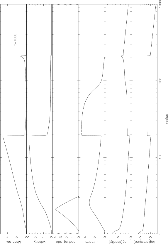
Figure 2: Results of a typical non-relativistic simulation at time $t=1000$ (where units of time are the dynamical time at the innermost radius, $\sqrt{R_{*}^{3}/GM}$). Quantities shown are the Mach number ($v/c_{s}$), velocity, heating rate ($\Lambda$), internal energy per unit mass ($u\equiv u_{\rm therm}$), log(density) and log(pressure).

We observe the effect of the heating propagating outwards in the atmosphere in the form of a shock front. After several hundred dynamical times the wind structure approaches a steady state in that there is only a small change of the overall wind structure due to the shock continuing to propagate outwards into the surrounding medium. The small disturbance propagating well ahead of the main shock is a transient resulting from the response of the atmosphere to the instantaneous switch-on of the heating. The velocity of the gas begins to asymptote to a constant value as the shock propagates outwards. Plotting the mass outflow rate $\dot{M}=4\pi r^{2}\rho v$ and the Bernoulli energy $E=\frac{1}{2}v^{2}+\rho u+P-GM/r$ as a function of radius (Figure 3),

Figure 3: Bernoulli energy $E=\frac{1}{2}v^{2}+\rho u+P-GM/r$ (top) and mass outflow rate $\dot{M}=4\pi r^{2}\rho v$ (bottom) in the time-dependent wind solution at $t=1000$. The profiles are approximately constant over the region between the two circles. The sample point used to match this flow to the appropriate steady state solution is indicated by a cross.

we see that indeed the wind structure is eventually close to that of a steady wind above the heating zone (ie. $\dot{M}$ and $E\sim$ constant). It is thus computationally inefficient and impractical to compute the time-dependent solution for long enough to determine an accurate velocity as $r\rightarrow\infty$ when the wind will continue to have a steady structure. Instead we find the steady wind solution for a given amount of energy input to the wind corresponding to the energy plotted in Figure 3 (top panel).

2.5 Steady wind solution

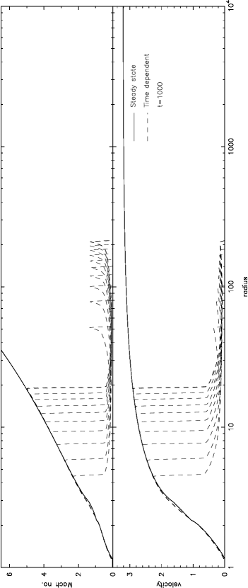
Figure 4: Steady wind Mach number (top panel) and velocity (centre panel) profiles are compared to the time-dependent solution (plotted every 100 dynamical times). There is a small discrepancy between the two solutions where we have taken the limit in approaching the singular point at $M=1$, but an otherwise excellent agreement between the two solutions.

Non-relativistic, steady state ($\partial/\partial t=0$) winds with energy input have been well studied by many authors, and the equations describing them can be found in Lamers & Cassinelli (1999), who credit the original work to Holzer & Axford (1970). The reader is thus referred to Lamers & Cassinelli (1999) for details of the derivation. As in the usual Bondi/Parker (Bondi 1952, Parker 1958) wind solution with no heat input, we set $\partial/\partial t=0$ in (1)-(5) and combine these equations into one equation for the Mach number $M^{2}=v^{2}/c_{s}^{2}$ as a function of radius, given by

$$\frac{dM^{2}}{dr}=-\frac{M^{2}(2+(\gamma-1)M^{2})}{2(M^{2}-1)\left[e(r)+GM/r\right]}\left[(1+M^{2}\gamma)\frac{dQ}{dr}+\frac{GM}{r^{2}}\frac{(5-3\gamma)}{(\gamma-1)}-\frac{4e(r)}{r}\right],$$ (11)

where $dQ/dr$ is the local heating gradient and $e(r)$ is the Bernoulli energy which is specified by integrating the Bernoulli equation

$$\frac{de(r)}{dr}=\frac{d}{dr}\left[\frac{1}{2}v^{2}+\rho u+P-\frac{GM}{r}\right]=\frac{dQ}{dr},$$ (12)

to give

$$e(r) = e(r_{\infty})-Q(r)$$ (13)

$$= e(r_{\infty})-\int^{r_{\infty}}_{r}\frac{dQ}{dr},$$

where $Q(r)$ is the total energy input to the wind. Since we are interested in the terminal velocity of the outflow we choose a point above the heating shell where the energy has reached its steady state value (i.e. where the energy is constant in Figure 3, top panel) and integrate outwards using the energy and Mach number at this point to solve (11) as an initial value problem. Note that in fact the terminal velocity is determined by the (constant) value of the Bernoulli energy above the heating zone since as $r\to\infty$, $e(r)\to\frac{1}{2}v^{2}$. However we compute the steady wind profiles both inwards and outwards to show the consistency between the time-dependent solution and the steady state version.

In order to perform the inward integration, we must determine the energy at every point for our steady solution by subtracting the heat input from the steady state energy as we integrate inwards through the heating shell (13). To determine this however we must also determine the local (steady state) heating gradient $dQ/dr$, which is related to the (time dependent) heating rate $\Lambda$ by setting $\partial/\partial t=0$ in the time dependent version, ie.

$$\Lambda=\frac{dQ}{dt}=\frac{\partial Q}{\partial t}+v\frac{dQ}{dr}=v\frac{dQ}{dr}.$$ (14)

We therefore calculate $dQ/dr$ from the time dependent solution using

$$\frac{dQ}{dr}=\frac{\Lambda(r)}{v(r)},$$ (15)

where $v(r)$ is the wind velocity at each point in the heating shell from the time-dependent solution. The problem with this is that at the inner edge of the heating shell the heating rate is finite while the velocity is very close to zero, resulting in a slight overestimate of the total energy input near the inner edge of the shell in the steady wind solution. Care must also be taken in integrating through the singular point in equation (11) at $M^{2}=1$. Most authors (e.g. Lamers & Cassinelli 1999) solve the steady wind equations starting from this point but for our purposes it is better to start the integration outside of the heating shell where the energy is well determined. We integrate through the critical point by using a first order Taylor expansion and appropriate limit(s), although this introduces a small discrepancy between the steady state and time-dependent results in this region (Figure 4).

Having determined the energy and heating gradient at each point in the wind we integrate (11) both inwards and outwards from the chosen point above the heating shell using a fourth order Runge-Kutta integrator (scaling (11) to the units described in §2.1.1). The velocity profile is then given by $v^{2}=M^{2}c_{s}^{2}$ where

$$c_{s}^{2}(r)=\frac{2(\gamma-1)}{2+M^{2}(r)(\gamma-1)}\left[e(r)+\frac{GM}{r}\right].$$ (16)

The resulting steady wind solution is shown in Figure 4 along with the time-dependent solution. The two profiles are in excellent agreement, proving the validity of our time-dependent numerical solution and the assumption that the wind is in a steady state. The steady solution thus provides an accurate estimate of the velocity at arbitrarily large radii (although as pointed out previously this is set by the value of the steady state Bernoulli energy).

2.6 Terminal wind velocities as a function of heating rate

Using the steady wind extrapolation of the time-dependent solution, we can determine the relationship between the heating rate and the terminal wind velocities. In order to make a useful comparison between the heating rates used in both the Newtonian and the relativistic regimes, we need to define a local canonical heating rate $\Lambda_{c}(r)$ valid in both sets of regimes. In dimensional terms the heating rate $\Lambda(r)$ corresponds to an input energy per unit mass per unit time. Thus we need to define the local canonical heating rate as

$$\Lambda_{c}(r)=\frac{\Delta E}{\Delta t},$$ (17)

for some relevant energy $\Delta E$ and some relevant timescale $\Delta t$.

There are clearly many different ways in which we might define a canonical heating rate. We find, however, that our results are not sensitive to the particular choice we make. We shall make use of a definition which draws on the physical processes we expect to be behind the jet acceleration process. Even though the processes by which this occurs are still obscure, we expect the energy for the jet to be provided fundamentally by liberation of energy in a rotating flow. Thus, with this physical motivation in mind, we take the canonical energy per unit mass, $\Delta E$, to be the energy released locally by bringing to rest a particle of unit mass which is orbiting in a circular orbit at radius $r$. In the Newtonian regime this is simply the kinetic energy of a circular orbit

$$\Delta E=\frac{1}{2}v_{\phi}^{2}=\frac{GM}{2r}.$$ (18)

(An alternative possibility, for example, would be to take $\Delta E$ to be the energy released by dropping a particle from infinity and bringing it to rest at radius $r$, which would correspond to the escape energy from that radius, $GM/r$.) By similar reasoning, we take the canonical timescale on which the energy is released to be the orbital timescale at radius $r$, that is $\Delta t=\Omega_{o}^{-1}$, where

$$\Omega_{o}=(GM/r^{3})^{1/2}.$$ (19)

Using this, we are now in a position to define a local canonical heating rate as

$$\Lambda_{c}(r)=\Delta E\times\Omega_{o}=\frac{(GM)^{3/2}}{2r^{5/2}}.$$ (20)

For intercomparison of our various wind computations both in the Newtonian and in the relativistic regimes, we now use the canonical heating rate derived above to define a dimensionless heating rate for each wind computation. Because heat is added over a range of radii, we need to define the dimensionless heating rate $\langle\Lambda\rangle$ as an appropriate volume average. We shall define

$$\langle\Lambda\rangle=\frac{\int^{r_{2}}_{r_{1}}\Lambda r^{2}dr}{\Lambda_{c}(r_{\rm max})\int^{r_{2}}_{r_{1}}r^{2}dr},$$ (21)

where $r_{\rm max}$ is the radius at which the heating rate $\Lambda(r)$ takes its maximum value and $r_{1}$ and $r_{2}$ are the lower and upper bounds of the heating shell respectively.

The relation between this average dimensionless heating rate and the terminal wind velocity is shown in Figure 5. The wind velocities are plotted in units of the escape velocity $v_{\rm esc}$ at $R_{*}$ and solutions are computed for wind velocities of up to $\sim 3v_{\rm esc}$. The important point in the present analysis is that the heating rate can be meaningfully compared to the relativistic results (see below).

Figure 5: Terminal wind velocities plotted as a function of the average dimensionless heating rate $\langle\Lambda\rangle$. Wind velocities are plotted in units of the escape velocity at the inner radius (ie. $r=R_{*}=1$), $v_{\rm esc}=(2GM/R_{*})^{1/2}$. We compute solutions corresponding to velocities typically observed in YSO jets (with a fairly generous upper limit of $v/v_{\rm esc}\sim 3$).

3 Relativistic jets

Having determined the heating rates required to produce the observed velocities in YSO jets we wish to perform exactly the same calculation within a relativistic framework. We proceed in precisely the same manner as in the non-relativistic case. We adopt the usual convention that Greek indices run over the four dimensions 0,1,2,3 while Latin indices run over the three spatial dimensions 1,2,3. Repeated indices imply a summation and a semicolon refers to the covariant derivative. The density $\rho$ refers to the rest mass density only, that is $\rho=nm_{0}$ where $n$ is the number density of baryons and $m_{0}$ is the mass per baryon.

3.1 Fluid equations

The equations describing a relativistic fluid are derived from the conservation of baryon number,

$$(\rho U^{\mu})_{;\mu}=0,$$ (22)

the conservation of energy-momentum projected along a direction perpendicular to the four velocity $U^{\mu}$ (which gives the equation of motion),

$$h_{\mu\alpha}T^{\alpha\nu}_{\phantom{\alpha\nu};\nu}=(g_{\mu\alpha}+U_{\mu}U_{\alpha})T^{\alpha\nu}_{\phantom{\alpha\nu};\nu}=0,$$ (23)

and projected in the direction of the four-velocity (which gives the energy equation),

$$U_{\alpha}T^{\alpha\nu}_{\phantom{\alpha\nu};\nu}=0.$$ (24)

Here the quantity $T^{\mu\nu}$ is the energy momentum tensor, which for a perfect fluid is given by

$$c^{2}T^{\mu\nu}=\rho hU^{\mu}U^{\nu}+Pg^{\mu\nu},$$ (25)

where $h$ is the specific enthalpy,

$$h=c^{2}+u+\frac{P}{\rho}=c^{2}+\frac{\gamma P}{(\gamma-1)\rho}.$$ (26)

As in the non-relativistic case $u$ is the internal energy per unit mass, $P$ is the gas pressure and we have used the equation of state given by equation (5). The energy equation may also be derived from the first law of thermodynamics using equation (22), which is a more convenient way of deriving an energy equation in terms of the internal energy (rather than the total energy) and in this case ensures that the meaning of the heating term is clear. The metric tensor is given by the Schwarzschild (exterior) solution to Einstein’s equations, that is

$$ds^{2}=-c^{2}d\tau^{2}=-\left(1-\frac{2GM}{c^{2}r}\right)c^{2}dt^{2}+\left(1-\frac{2GM}{c^{2}r}\right)^{-1}dr^{2}+r^{2}(d\theta^{2}+\mathrm{sin}^{2}\theta d\phi^{2}).$$ (27)

We consider radial flow such that $U^{\theta}=U^{\phi}=0$. The four velocity is normalised such that

$$U_{\mu}U^{\mu}=-c^{2},$$ (28)

and we define

$$U^{t}\equiv\frac{dt}{d\tau}=\left(1-\frac{2GM}{c^{2}r}\right)^{-1}\left[\left(1-\frac{2GM}{c^{2}r}\right)+\frac{(U^{r})^{2}}{c^{2}}\right]^{1/2},$$ (29)

which we denote as

$$U^{t}=\frac{\Gamma}{\alpha^{2}}$$ (30)

where we set for convenience

$$\Gamma=\left[\left(1-\frac{2GM}{c^{2}r}\right)+\frac{(U^{r})^{2}}{c^{2}}\right]^{1/2},$$ (31)

and

$$\alpha^{2}=\left(1-\frac{2GM}{c^{2}r}\right).$$ (32)

Note that while $\alpha$ corresponds to the lapse function in the $3+1$ formulation of general relativity, the quantity $\Gamma$ is not the Lorentz factor of the gas (which we denote as $W$) as it is usually defined in numerical relativity (e.g. Banyuls et al. 1997) but is related to it by $W=\Gamma/\alpha$. From (29) we also have the relation

$$\frac{\partial U^{t}}{\partial t}=\frac{U^{r}}{\alpha^{2}\Gamma c^{2}}\frac{\partial U^{r}}{\partial t}$$ (33)

From (22), (23) and (24) using (25), (27), (29) and (33) we thus derive the continuity equation,

$$\frac{\partial\rho}{\partial t}+v^{r}\frac{\partial\rho}{\partial r}+\frac{\alpha^{2}\rho}{\Gamma}\left[\frac{1}{r^{2}}\frac{\partial}{\partial r}(r^{2}U^{r})+\frac{U^{r}}{\alpha^{2}\Gamma c^{2}}\frac{\partial U^{r}}{\partial t}\right]=0,$$ (34)

the equation of motion,

$$\frac{\partial U^{r}}{\partial t}+v^{r}\frac{\partial U^{r}}{\partial r}+\frac{\Gamma\alpha^{2}c^{2}}{\rho h}\frac{\partial P}{\partial r}+\frac{U^{r}}{\rho h}\frac{\partial P}{\partial t}+\frac{\alpha^{2}}{\Gamma}\frac{GM}{r^{2}}=0,$$ (35)

and the internal energy equation,

$$\frac{\partial(\rho u)}{\partial t}+v^{r}\frac{\partial(\rho u)}{\partial r}+\frac{\alpha^{2}}{\Gamma}\left(P+\rho u\right)\left[\frac{1}{r^{2}}\frac{\partial}{\partial r}(r^{2}U^{r})+\frac{U^{r}}{\alpha^{2}\Gamma c^{2}}\frac{\partial U^{r}}{\partial t}\right]=\frac{\alpha^{2}}{\Gamma}\rho\Lambda,$$ (36)

where

$$v^{r}\equiv\frac{U^{r}}{U^{t}}\equiv\frac{dr}{dt}$$ (37)

is the velocity in the co-ordinate basis. We define the heating rate per unit mass as

$$\Lambda\equiv T\frac{ds}{d\tau},$$ (38)

where $T$ is the temperature, $s$ is the specific entropy and $d\tau$ refers to the local proper time interval ($\Lambda$ is therefore a local rate of energy input, caused by local physics). A comparison of (34), (35) and (36) with their non-relativistic counterparts (1), (2) and (3) shows that they reduce to the non-relativistic expressions in the limit as $c\to\infty$, and to special relativity as $M\to 0$.

The ‘source terms’ containing time derivatives of $U^{r}$ and $P$ are then eliminated between the three equations using the equation of state (5) to relate pressure and internal energy. Substituting for pressure in (36) and substituting this into (35) we obtain the equation of motion in terms of known variables,

$$\frac{\partial U^{r}}{\partial t}+\frac{v^{r}}{X}\left(1-\frac{\gamma P}{\rho h}\right)\frac{\partial U^{r}}{\partial r}=-\frac{c^{2}\alpha^{4}}{\rho h\Gamma X}\frac{\partial P}{\partial r}-\frac{\alpha^{2}}{\Gamma X}\frac{GM}{r^{2}}+\frac{v^{r}}{X}\frac{\gamma P}{\rho h}\frac{2U^{r}}{r}-\frac{v^{r}}{hX}(\gamma-1)\Lambda,$$ (39)

where for convenience we define

$$X\equiv 1-\left(\frac{\gamma P}{\rho h}\right)\frac{U^{r}U^{r}}{\Gamma^{2}c^{2}},$$ (40)

and we have expanded the $\frac{1}{r^{2}}\frac{\partial}{\partial r}(r^{2}U^{r})$ terms in order to combine the spatial derivatives of $U^{r}$ into one term. We then substitute (39) into (34) and (36) to obtain equations for the density

$$\frac{\partial\rho}{\partial t}+v^{r}\frac{\partial\rho}{\partial r}=-\frac{\alpha^{2}}{\Gamma}\left[\rho A-\frac{v^{r}}{h\Gamma X}\frac{\partial P}{\partial r}-\frac{U^{r}U^{r}}{\Gamma^{2}c^{2}X}\frac{(\gamma-1)}{h}\rho\Lambda\right],$$ (41)

and internal energy,

$$\frac{\partial(\rho u)}{\partial t}+v^{r}\left(1-\frac{\gamma P}{\rho h}\frac{\alpha^{2}}{\Gamma^{2}X}\right)\frac{\partial(\rho u)}{\partial r}=-\frac{\alpha^{2}}{\Gamma}\left[(P+\rho u)A-\left(1+\frac{U^{r}U^{r}}{\Gamma^{2}c^{2}X}\frac{\gamma P}{\rho h}\right)\rho\Lambda\right].$$ (42)

where for convenience we have defined

$$A\equiv\left[1-\frac{U^{r}U^{r}}{\Gamma^{2}c^{2}X}\left(1-\frac{\gamma P}{\rho h}\right)\right]\frac{\partial U^{r}}{\partial r}+\left[1+\frac{U^{r}U^{r}}{\Gamma^{2}c^{2}X}\left(\frac{\gamma P}{\rho h}\right)\right]\frac{2U^{r}}{r}-\frac{U^{r}}{\Gamma^{2}c^{2}X}\frac{GM}{r^{2}}$$ (43)

From the solution specifying $U^{r}$ we calculate the velocity measured by an observer at rest with respect to the time slice (referred to as Eulerian observers), which is given by

$$\bar{v}^{r}=\frac{U^{r}}{\alpha U^{t}}=\frac{v^{r}}{\alpha},$$ (44)

since there are no off-diagonal terms (ie. zero shift vector) in the Schwarzschild solution. For these observers the Lorentz factor is given by

$$W=\left(1-\frac{\bar{v}^{r}\bar{v}_{r}}{c^{2}}\right)^{-1/2},$$ (45)

where $\bar{v}^{r}\bar{v}_{r}=g_{rr}\bar{v}^{r}\bar{v}^{r}$, such that $U^{r}=W\bar{v}^{r}$.

3.2 Scaling

The usual practice in numerical relativity is to scale in so-called geometric units such that $G=M=c=1$. In these units the length scale would be the geometric radius $GM/c^{2}$ and the velocity would have units of $c$. Instead for the current problem, we adopt a scaling analogous to that of the non-relativistic case, that is we choose the length scale to be the radius of the central object, $R_{*}$, where $R_{*}$ is given as some multiple of the geometric radius, ie.

$$[L]=R_{*}=n\frac{GM_{*}}{c^{2}},$$ (46)

with $n\geq 2.0$. The mass scale is again the central object mass $[M]=M_{*}$ and the timescale is given by

$$[\tau]=\left(\frac{GM_{*}}{R_{*}^{3}}\right)^{-1/2}=n^{3/2}\frac{GM_{*}}{c^{3}}$$ (47)

In these units, velocity is measured in units of $[v]=n^{-1/2}c$ (or equivalently $c^{2}=n$). The scaled equations are thus given simply by setting $G=M=1$ and $c^{2}=n$ everywhere.

This scaling ensures that the relativistic terms tend to zero when $c$ (or $n$) is large and that the numerical values of $\rho$, $\rho u$ and $U^{r}$ are of order unity. We thus specify the degree to which the gravity/gas dynamics is relativistic by specifying the value of $n$ (i.e. the proximity of the innermost radius, and thus the heating, to the Schwarzschild radius, $R_{\rm Sch}=2GM/c^{2}$). We compute solutions corresponding to gas very close to a black hole (highly relativistic, $n=2.0$, or $R_{*}=R_{\rm Sch}$), neutron star (moderately relativistic, $n=5$, or $R_{*}=R_{\rm NS}=5GM/c^{2}$, which is equivalent to heating further out and over a wider region around a black hole) and white dwarf/non-relativistic star (essentially non-relativistic, $n=5000$, or $R_{*}=2500R_{\rm Sch}$). Note that in the highly relativistic case although we scale the solution to $n=2.0$ such that the mass, length and time scales (and therefore the units of heating rate, energy etc.) correspond to those at $r=R_{\rm Sch}$, our numerical grid cannot begin at $R_{*}$ as it does in the other cases. We therefore set the lower bound on the radial grid to slightly below the heating shell (typically $r=1.01R_{*}$ where the heating begins at $1.1R_{*}$). Note that the above scaling is merely to ensure that the numerical solution is of order unity, since we scale in terms of dimensionless variables to compare with the non-relativistic solution.

3.3 Numerical Solution

In order to solve the relativistic fluid equations numerically we use a method analogous to that used in the non-relativistic case (Figure 11). That is, we first compute $U^{r}$ on the staggered (half) grid and use this to solve for $\rho$ and $\rho u$ on the integer grid points. Again the advective terms are discretized using upwind differences (where the ‘upwindedness’ is determined from the sign of the co-ordinate velocity $v^{r}$) and other derivatives are calculated using centred differences. As in the non-relativistic case, where a centred difference is used, the quantities multiplying the derivative are interpolated onto the half grid points if necessary. In equation (41) we evaluate the $\partial P/\partial r$ term using upwind differences.

3.4 Initial Conditions

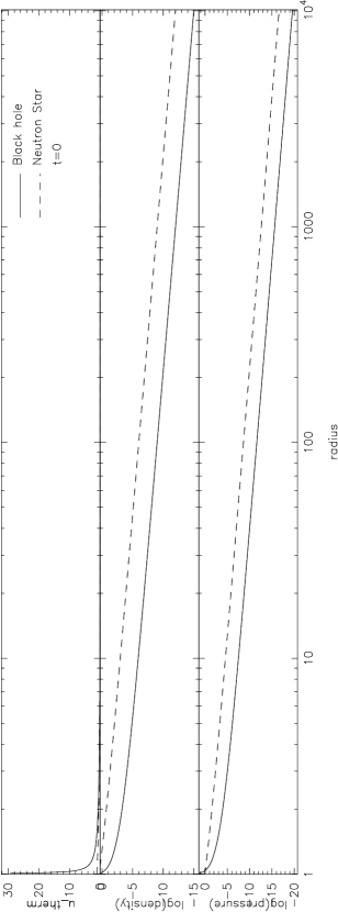
Figure 6: The initial conditions for the gas reservoir for the relativistic cases of a neutron star (dashed line) ($R_{*}/R_{\rm Sch}=2.5$) and black hole (solid line)($R_{*}/R_{\rm Sch}=1.0$). Note, however, that the innermost radius is at $r=1.01R_{*}$ in the latter case. We plot profiles of internal energy per unit mass (or temperature), density and pressure, as functions of radius. These quantities are given in units of $GM/R_{*}$, $M/R_{*}^{3}$ and $M_{*}/(R_{*}t_{*}^{2})$ respectively. Note that steeper gradients are required to hold the gas in hydrostatic equilibrium as the gravitational field becomes more relativistic. The black hole reservoir is of lower density than the neutron star version because of the choice of the polytropic constant (chosen such that the central density is of order unity).

We determine initial conditions for the relativistic case by setting $U^{r}=0$ and $\partial/\partial t=0$ in (39), from which we have

$$\frac{dP}{dr}=-\frac{\rho h}{c^{2}}\frac{GM}{r^{2}}\left(1-\frac{2GM}{c^{2}r}\right)^{-1}.$$ (48)

The pressure is thus calculated as a function of $\rho$, $u$ and $P$ (where $P=(\gamma-1)\rho u$). We solve (48) using the same assumptions as in the non-relativistic case (§2.3), that is an adiabatic atmosphere such that

$$P=K\rho^{\gamma}.$$ (49)

We therefore have

$$\frac{d\rho}{dr}=-\frac{1}{\gamma K\alpha^{2}}\left[\rho^{(2-\gamma)}+\frac{\gamma K\rho}{c^{2}(\gamma-1)}\right]\frac{GM}{r^{2}},$$ (50)

which we solve using a first order (Euler) discretization to obtain a density profile. The pressure may then be calculated using (49), however to ensure that hydrostatic equilibrium is enforced numerically we solve (48) using the same discretization as in the fluid equations, integrating inwards from the outer boundary condition $P(r_{\rm max})=K\rho(r_{\rm max})^{\gamma}$. However in this case the pressure gradient also depends on the pressure, so we use the pressure calculated from (49) to calculate the initial value of the specific enthalpy $h$ and iterate the solution until converged ($[P^{n+1}-P^{n}]/P^{n}<10^{-10}$). In the black hole case the resulting pressure differs from that found using (49) by $\Delta P/P\sim 10^{-2}$. We choose $K$ such that the central density is of order unity – typically we use $K=10\gamma/(\gamma-1)$ in the black hole case. Note that changing $K$ simply changes the amount of matter present in the atmosphere but does not affect the temperature scaling and does not affect the final results (although it significantly affects the integration time since it determines the strength of the shock front and the amount of mass to be accelerated).

Initial conditions calculated in this manner for the black hole ($R_{*}/R_{\rm Sch}=n/2=1.0$) and neutron star ($R_{*}/R_{\rm Sch}=2.5$) atmospheres are shown in Figure 6. The initial setup reduces to that of Figure 1 in the non-relativistic limit when the same value of $K$ is used. We set the outer boundary at $r/R_{*}=10^{4}$, using 1335 radial grid points (again on a logarithmic grid).

3.5 Results

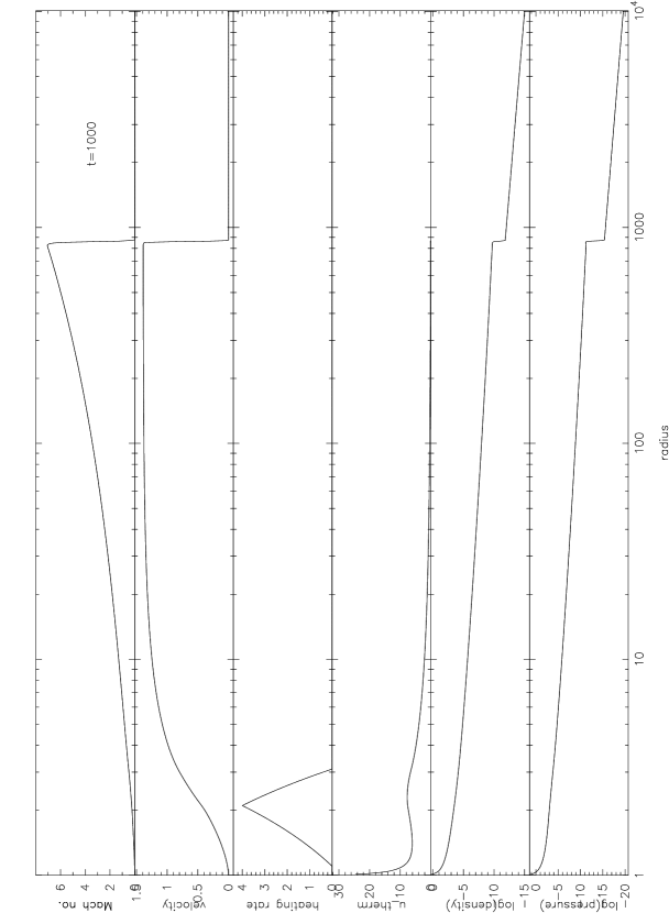
Figure 7: Results of a typical black hole relativistic simulation at t=1000 (where units of time are the dynamical time at the central object). Quantities shown are the Mach number ($v/c_{s}$), velocity for Eulerian observers ($\bar{v}^{r}$), heating rate ($\Lambda$), internal energy per unit mass ($u\equiv u_{\rm therm}$), log(density) and log(pressure). Units of velocity are such that $c=\sqrt{2}$ and as in the non-relativistic case energy has units of $GM/R_{*}$.

Figure 8: The relativistic Bernoulli energy $E_{\rm rel}=\frac{1}{2}\Gamma h/c^{2}-\frac{1}{2}c^{2}$(top) and mass outflow rate $\dot{M}=4\pi r^{2}\rho U^{r}$ (bottom) in the time-dependent relativistic wind solution with a reasonably high heating rate are shown as functions of radius at time $t=1000$. In order to match this solution to a steady outflow solution, the Bernoulli energy is assumed to be constant over the region indicated by the two circles, and the steady wind solution is computed using initial values at the point indicated by a cross.

The results of a typical (n=2.0) relativistic simulation are shown in Figure 7 at $t=1000$. Again we observe that the wind structure reaches a quasi-steady state, with the velocity approaching a steady value at large radii. Note that because the steady state density is higher than that of the surrounding medium no wide shock front is observed.

Plotting the mass outflow rate $\dot{M}=4\pi r^{2}\rho U^{r}$ and the relativistic Bernoulli energy $E_{\rm rel}=\frac{1}{2}\Gamma^{2}h^{2}/c^{2}-\frac{1}{2}c^{2}$ (see e.g. Shapiro & Teukolsky 1983) as a function of radius (Figure 8), we see that indeed the structure approaches that of a steady (relativistic) wind (that is, the energy and $\dot{M}$ profiles are flat above the heating zone). We may thus apply a relativistic steady wind solution with this Bernoulli energy as an initial value to determine the final velocity and Lorentz factor as $r\rightarrow\infty$. Note that we cannot apply a non-relativistic steady wind solution because although the gravity is non-relativistic, the outflow velocities are not. As in the non-relativistic case the final wind velocity is determined by the steady Bernoulli energy, since in this case as $r\rightarrow\infty$, $E_{\rm rel}\rightarrow\frac{1}{2}[(U^{r})^{2}-c^{2}]$.

3.6 Steady wind solution

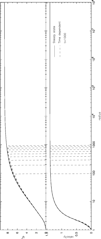
Figure 9: The radial profiles of the steady wind r-component of four velocity $U^{r}$ (top panel) and of the velocity for Eulerian observers $\bar{v}^{r}$ (centre panel) are compared to the time-dependent solution (plotted every 100 dynamical times) for a typical relativistic calculation for the black hole (n=2.0) case. Units are such that $c=\sqrt{2}$ on the velocity plots. Note the excellent agreement between the two solutions.

Relativistic, steady state ($\partial/\partial t=0$) winds were first studied by Michel (1972) and extended to include energy deposition by Flammang (1982). The problem has recently received attention in the context of neutrino-driven winds in gamma-ray burst models by Pruet, Fuller & Cardall (2001) and Thompson, Burrows & Meyer (2001). We proceed in a manner analogous to that of the non-relativistic solution. Setting $\partial/\partial t=0$ the continuity (22) and momentum (23) equations become

$$\frac{1}{\rho}\frac{\partial\rho}{\partial r}+\frac{1}{U^{r}}\frac{\partial U^{r}}{\partial r}+\frac{2}{r} = 0$$ (51)

$$U^{r}\frac{\partial U^{r}}{\partial r}+\frac{\Gamma^{2}c^{2}}{\rho h}\frac{\partial P}{\partial r}+\frac{GM}{r^{2}} = 0$$ (52)

where (51) is equivalent to

$$r^{2}\rho U^{r}=\mathrm{const}.$$ (53)

Combining (52) and (51) we obtain

$$\frac{1}{U^{r}}\left[(U^{r})^{2}-\frac{c^{2}\Gamma^{2}c_{s}^{2}}{h\gamma}\right]\frac{\partial U^{r}}{\partial r}=-\frac{c^{2}\Gamma^{2}}{h\gamma}\frac{dc_{s}^{2}}{dr}+\frac{c^{2}\Gamma^{2}}{h\gamma}\frac{2c_{s}^{2}}{r}-\frac{GM}{r^{2}},$$ (54)

where $c_{s}^{2}=\gamma P/\rho$ and $(U^{r})^{2}\equiv U^{r}U^{r}$. From the first law of thermodynamics and (52) we derive the relativistic Bernoulli equation in the form

$$\frac{d}{dr}\left(\frac{1}{2}\frac{\Gamma^{2}h^{2}}{c^{2}}\right)=\frac{h\Gamma^{2}}{c^{2}}\frac{dQ}{dr},$$ (55)

such that both sides reduce to their non-relativistic expressions as $c\to\infty$. The quantity $dQ/dr$ is the local heating gradient as in the non-relativistic case. Expanding this equation we find

$$\frac{dc_{s}^{2}}{dr}=(\gamma-1)\left[\frac{dQ}{dr}-\frac{h}{c^{2}\Gamma^{2}}\frac{d}{dr}\left(\frac{1}{2}(U^{r})^{2}\right)-\frac{h}{c^{2}\Gamma^{2}}\frac{GM}{r^{2}}\right].$$ (56)

Combining (56) and (54) and manipulating terms, we obtain an equation for $(U^{r})^{2}$,

$$\frac{d}{dr}(U^{r})^{2}=\frac{2(U^{r})^{2}}{\left[(U^{r})^{2}-c^{2}\Gamma^{2}c_{s}^{2}/h\right]}\left[\frac{c^{2}\Gamma^{2}}{h}\frac{2c_{s}^{2}}{r}-(\gamma-1)\frac{c^{2}\Gamma}{h}\left(\Gamma\frac{dQ}{dr}\right)-\frac{GM}{r^{2}}\right],$$ (57)

where $c_{s}^{2}$ and $h=c^{2}+c_{s}^{2}/(\gamma-1)$ are given functions of known variables by integration of the Bernoulli equation (55), in the form

$$\frac{d}{dr}\left(\Gamma h\right)=\Gamma\frac{dQ}{dr},$$ (58)

to ensure that $h$ does not appear in the heating term on the right hand side. The integration is then

$$e(r)=\Gamma h=e(r_{\infty})-\int^{r_{\infty}}_{r}\left\{\Gamma\frac{dQ}{dr}\right\}dr,$$ (59)

and hence

$$h=\frac{e(r)}{\Gamma},\hskip 14.22636ptc_{s}^{2}=(\gamma-1)(h-c^{2}).$$ (60)

The ‘heating gradient’, $\Gamma dQ/dr$, is calculated from the time-dependent solution using

$$\Gamma\frac{dQ}{dr}(r)=\frac{\alpha(r)\Lambda(r)}{\bar{v}^{r}(r)},$$ (61)

since

$$\Lambda\equiv T\frac{ds}{d\tau}\equiv\frac{dQ}{d\tau}=U^{t}\left(\frac{\partial Q}{\partial t}+v^{r}\frac{dQ}{dr}\right),$$ (62)

where $\tau$ is the proper time and $U^{t}=\Gamma/\alpha^{2}$. The velocity profile for an Eulerian observer is then calculated using (44) and the final Lorentz factor $W_{\infty}$ using equation (45). As in the non-relativistic case we choose a starting point for the integration above the heating shell and integrate outwards from this point using a fourth order Runge-Kutta integrator in order to determine the terminal Lorentz factor. The inward integration (and thus the determination of the steady state heating gradient $\Gamma dQ/dr$) is computed only for consistency. We integrate through the singular point in equation (57) by taking a low order integration with larger steps as this point is approached.

The solution calculated using (57) is shown in Figure 9 plotted against the evolving time-dependent solution. The profiles are in excellent agreement, verifying the accuracy of the relativistic calculation and showing that the wind may indeed be described by the steady state solution.

3.7 Terminal wind velocities and Lorentz factors as a function of heating rate

Figure 10: The terminal r-component of four velocity $U^{r}$ (top panel) and Lorentz factor (bottom panel) of the wind in the non-relativistic ($\circ$, solid), white dwarf ($\times$, dot-dashed), neutron star ($+$, dotted) and black hole ($*$, dashed) cases, is plotted as a function of the dimensionless heating rate defined in $\S\ref{sec:nrrates}$. The top panel may be compared with Figure 5 in the non-relativistic case.

In order to compare the relativistic results to those in the Newtonian regime, we define the local canonical heating rate in a similar manner to the non-relativistic case, that is

$$\Lambda_{c}(r)=\frac{\Delta E}{\Delta t},$$ (63)

for some relevant energy $\Delta E$ and some relevant timescale $\Delta t$. As in Section 2.6 we take the canonical energy per unit mass, $\Delta E$, to be the energy released locally by bringing to rest a particle of unit mass which is orbiting in a circular orbit at radius $r$. For a particle orbiting in the Schwarzschild metric this is the difference, $\Delta E$, between the energy constants (defined by the timelike Killing vector) of a circular geodesic at radius $r$, and a radial geodesic with zero velocity at radius $r$. This implies (see, for example, Schutz 1990, Chapter 11)

$$\Delta E/c^{2}=\frac{1-2GM/rc^{2}}{[1-3GM/rc^{2}]^{1/2}}-[1-2GM/rc^{2}]^{1/2}.$$ (64)

In the Newtonian limit, this reduces to the expected value $\Delta E=\frac{1}{2}v_{\phi}^{2}=GM/2r$. We again take the canonical timescale on which the energy is released to be the orbital timescale at radius $r$ as measured by a local stationary observer. For a circular geodesic in the Schwarzschild metric, the azimuthal velocity is given in terms of coordinate time, $t$, by

$$d\phi/dt=\Omega=(GM/r^{3})^{1/2}.$$ (65)

This is the same expression as for the angular velocity of an orbiting particle in the Newtonian limit. But in terms of the proper time, $\tau$, of a local stationary observer we have, from the metric,

$$d\tau/dt=(1-2GM/rc^{2})^{1/2},$$ (66)

and thus $d\phi/d\tau=\Omega_{o}$, where

$$\Omega_{o}^{2}=\frac{GM}{r^{3}}\left[1-\frac{2GM}{rc^{2}}\right]^{-1}.$$ (67)

Using this, the local canonical heating rate is therefore given by

$$\Lambda_{c}=\Delta E\times\Omega_{o}.$$ (68)

In the Newtonian limit, $r\gg 2GM/c^{2}$, this becomes as expected $\Lambda_{c}\simeq(GM)^{3/2}/2r^{5/2}$. As in the non-relativistic case we use the canonical heating rate derived above to define a dimensionless heating rate $\langle\Lambda\rangle$ as an appropriate volume average using equation (21).

The final Lorentz factor of the wind plotted as a function of this dimensionless heating rate is given in the bottom panel of Figure 10 in the highly relativistic (black hole), moderately relativistic (neutron star, equivalent to a broader heating shell further away from a black hole) and non-relativistic (white dwarf) cases.

We would also like to make a meaningful comparison of the final wind velocities in units of the escape velocity from the star. Note that we cannot simply compare the scaled velocities since we are in effect introducing a ‘speed limit’ in the relativistic solution such that the (scaled) relativistic velocity will always be slower than in the equivalent non-relativistic solution. However we can compare the velocity for observers along the worldline of a particle in the wind (ie. observers with proper time interval $d\tau$), $U^{r}=dr/d\tau$ (that is, the $r$ component of the four velocity, which in special relativity is given by $U^{r}=\gamma v^{r}$, where $\gamma$ is the Lorentz factor). Scaling this in units of the (Newtonian) escape velocity from the central object $(2GM/R_{*})^{1/2}$ we can make a useful comparison with the non-relativistic results. This velocity is plotted in the top panel of Figure 10 against the dimensionless heating rate.

4 Discussion and Conclusions

We have considered the input of energy at the base of an initially hydrostatic atmosphere as a simple model for the acceleration of an outflow or jet. The problem is inherently a time-dependent one, because the flow velocity at the base of the atmosphere is zero. Sufficiently large energy input rates give rise to supersonic outflows. We are, of course, unable to compute the outflow for an infinite time, and thus cannot directly measure the terminal outflow speed. However, we make use of the fact that if the mass in the atmosphere is sufficiently large compared to the mass outflow rate, then at large radii the outflow approximates to a steady state (with constant mass flux). We thus match our time-dependent solutions onto steady state outflow solutions at large radii and thus determine the terminal velocities for the outflows. We then compute how the terminal velocity of the outflow varies as a function of (dimensionless) heating rate in both Newtonian and relativistic gravitational potentials. The results are shown in Figures 5 and 10.

In the top half of Figure 10 we note that dimensionless energy (or momentum) imparted to the outflow at a given value of the dimensionless heating rate is larger in the relativistic regime. This comes about simply because a particular element of gas cannot escape from the zone in which the heating is occurring with a velocity which exceeds the speed of light. Thus a gas element which is accelerated to relativistic energies in the heating zone spends longer in the heating zone than one which is not. Indeed from Figure 10, we see that, once the outflows become relativistic, the energy per unit mass in the outflow (proportional to $\gamma$) is proportional to the dimensionless heating rate $\langle\Lambda\rangle$. This comes about because each fluid element spends the same time in the heating zone, because it travels through the zone at a velocity $\sim c$.

From Figure 5 we see that a dimensionless heating rate of $\langle\Lambda\rangle\simeq 17$ gives rise to a terminal outflow velocity of $v_{\rm jet}\simeq 2v_{\rm esc}$ in a Newtonian potential. From Figure 10, we see that for the same heating rate, the ‘neutron star’ wind, for which the heating rate peaks at about 5.2 $R_{\rm Sch}$ becomes mildly relativistic ($\gamma_{\rm jet}\sim 2$), whereas the ‘black hole’ wind, for which the heating rate peaks at about 2.1 $R_{\rm Sch}$, leads to an outflow with $\gamma_{\rm jet}\simeq 11$. Similarly a dimensionless heating rate of $\langle\Lambda\rangle\simeq 55$ gives rise to a terminal velocity of $v_{\rm jet}\simeq 3v_{\rm esc}$ in the Newtonian case, to an outflow with $\gamma_{\rm jet}\sim 4$ in the mildly relativistic case, and to an outflow with $\gamma_{\rm jet}\simeq 31$ in the strongly relativistic case. We have noted above that although the exact numerical values here do depend slightly on the exact definition of the dimensionless heating rate, the basic results remain unchanged. For example, using the Newtonian dimensionless heating rate (§2.6) in the strongly relativistic case gives a Lorentz factor of $\gamma_{\rm jet}\simeq 5$ for the rate which corresponds to $v_{\rm jet}\simeq 2v_{\rm esc}$ in the non-relativistic case.

We caution that the above analysis does not demonstrate that the model we use provides an adequate description of the physics involved in the acceleration process (for example, the jet energy might be initially mainly in electromagnetic form – Poynting flux – and only later converted to kinetic energy of baryons) or that there is no intrinsic difference between the jet outflows caused by the relativistic nature of the AGN jets (for example, the AGN jets might be mainly in the form of a pair plasma and therefore lighter). And we note that it is evident that more detailed physical models need to be developed before further conclusions can be drawn. Nevertheless, we suggest that the generic nature of our analysis might give some insight into the physical processes involved in the acceleration of jets.

Thus we conclude, on the basis of the rather simplified physical model we have employed in our analysis, that it is not unreasonable to argue that the jets in AGN are simply scaled up, relativistic versions of the jets in YSOs, and that the intrinsic jet acceleration mechanism is indeed the same in both the AGN and the YSO contexts. In making this analogy, again on the basis of our simplified model for the acceleration process, we find two further physical conditions must hold. First, we find that the energy input process, which leads to the acceleration of the outflow, takes place deep in the (relativistic) gravitational well for the AGN case ($\sim 2R_{Sch}$). What this means physically is that in this way it is possible to make use of the limiting velocity, $c$, to ensure that relativistic fluid elements remain relatively longer in the energy input zone compared to their non-relativistic counterparts. Second, we find that the required dimensionless heating rate is much larger than unity. The physical implication of this is that the available energy released in the accretion process must be imparted to a small fraction of the available accreting material.

Appendix A Discretization scheme for non-relativistic equations

Figure 11: Schematic diagram of numerical method: density and internal energy are defined on the integer points while velocity is calculated on the half points. The solution requires one inner boundary condition on $v$ and two outer boundary conditions for $\rho$ and $\rho u$. Updated velocities ($v^{n+1}$) are used to calculate $\rho^{n+1}$ and $\rho u^{n+1}$. The scheme allows centred differencing on terms involving staggered quantities (top panel) while upwind differencing is used on the advective terms (bottom panel).

The discretization scheme for the non-relativistic fluid equations is summarised in Figure 11. Fluxes are calculated on the half grid points while the other terms are calculated on the integer points. We solve (1)-(5) in the following manner: The numerical equations are solved first for velocity on the half grid points (dropping the superscript $r$ for convenience),

$$v^{n+1}_{i+1/2} = v^{n+1}_{i+1/2}-\Delta t\left[v^{n}_{i+1/2}\left(\frac{v^{n}_{i+3/2}-v^{n}_{i+1/2}}{r_{i+3/2}-r_{i+1/2}}\right)-\frac{1}{\rho^{n}_{i+1/2}}\left(\frac{P^{n}_{i+1}-P^{n}_{i}}{r_{i+1}-r_{i}}\right)-\frac{1}{r^{2}_{i+1/2}}\right]\hskip 14.22636pt(v<0)$$ (69)

$$= v^{n+1}_{i+1/2}-\Delta t\left[v^{n}_{i+1/2}\left(\frac{v^{n}_{i+1/2}-v^{n}_{i-1/2}}{r_{i+3/2}-r_{i+1/2}}\right)-\frac{1}{\rho^{n}_{i+1/2}}\left(\frac{P^{n}_{i+1}-P^{n}_{i}}{r_{i+1}-r_{i}}\right)-\frac{1}{r^{2}_{i+1/2}}\right]\hskip 14.22636pt(v>0)$$

where the superscript $n$ refers to the $n$th timestep and the subscript $i$ refers to $i$th grid point ($v_{i+1/2}$,$\rho_{i+1/2}$ thus being points on the staggered velocity grid). The quantity $\rho_{i+1/2}$ is calculated using linear interpolation between the grid points, ie. $\rho_{i+1/2}=\frac{1}{2}(\rho_{i}+\rho_{i+1})$. We then solve for the density and internal energy on the integer grid points using the updated velocity,

$$\rho^{n+1}_{i} = \rho^{n}_{i}-\Delta t\left[v^{n+1}_{i}\left(\frac{\rho^{n}_{i+1}-\rho^{n}_{i}}{r_{i+1}-r_{i}}\right)-\frac{\rho_{i}^{n}}{r_{i}^{2}}\left(\frac{r^{2}_{i+1/2}v^{n+1}_{i+1/2}-r^{2}_{i-1/2}v^{n+1}_{i-1/2}}{r_{i+1/2}-r_{i-1/2}}\right)\right]\hskip 14.22636pt(v<0)$$ (70)

$$= \rho^{n}_{i}-\Delta t\left[v^{n+1}_{i}\left(\frac{\rho^{n}_{i}-\rho^{n}_{i-1}}{r_{i}-r_{i-1}}\right)-\frac{\rho_{i}^{n}}{r_{i}^{2}}\left(\frac{r^{2}_{i+1/2}v^{n+1}_{i+1/2}-r^{2}_{i-1/2}v^{n+1}_{i-1/2}}{r_{i+1/2}-r_{i-1/2}}\right)\right]\hskip 14.22636pt(v>0)$$

and similarly,

$$\rho u^{n+1}_{i} = \rho u^{n}_{i}-\Delta t\left[v^{n+1}_{i}\left(\frac{\rho u^{n}_{i+1}-\rho u^{n}_{i}}{r_{i+1}-r_{i}}\right)-\left[\frac{P_{i}^{n}+\rho u^{n}_{i}}{r_{i}^{2}}\right]\left(\frac{r^{2}_{i+1/2}v^{n+1}_{i+1/2}-r^{2}_{i-1/2}v^{n+1}_{i-1/2}}{r_{i+1/2}-r_{i-1/2}}\right)+\rho^{n}_{i}\Lambda_{i}\right]\hskip 14.22636pt(v<0)$$ (71)

$$= \rho u^{n}_{i}-\Delta t\left[v^{n+1}_{i}\left(\frac{\rho u^{n}_{i}-\rho u^{n}_{i-1}}{r_{i}-r_{i-1}}\right)-\left[\frac{P_{i}^{n}+\rho u^{n}_{i}}{r_{i}^{2}}\right]\left(\frac{r^{2}_{i+1/2}v^{n+1}_{i+1/2}-r^{2}_{i-1/2}v^{n+1}_{i-1/2}}{r_{i+1/2}-r_{i-1/2}}\right)+\rho^{n}_{i}\Lambda_{i}\right]\hskip 14.22636pt(v>0)$$

where $\Delta t=t^{n+1}-t^{n}$ and the timestep is regulated according to the Courant condition

$$\Delta t<\frac{\mathrm{min}(\Delta r)}{\mathrm{max}(\left|{v}\right|)+\mathrm{max}(c_{s})}$$ (72)

where $c_{s}$ is the adiabatic sound speed in the gas given by $c_{s}^{2}=\gamma P/\rho$. We typically set $\Delta t$ to half of this value.

References

- Bally et al. (2002) Bally, J., Heathcote, R., Reipurth, B., Morse, J., Hartigan, P., Schwartz, D., 2002, AJ, 123, 2627
- Bally et al. (2001) Bally, J., Johnstone, D., Joncas, G., Reipurth, B.,Mallén-Ornelas, G.,2002, AJ, 122, 1508
- Banyuls et al. (1997) Banyuls, F., Font, J. A., Ibañez, J. Ma., Marti, J.Ma., Miralles, J. A., 1997, ApJ, 476, 221
- Blandford (1993) Blandford, R. D., 1993, in Astrophysical Jets, eds. D. Burgarella, M. Livio, C. P. O’Dea, Cambridge University Press, p 15
- Blandford (2000) Blandford, R. D., 2000, Phil. Trans. Roy. Soc. Lond., 358, 811
- Blandford (2002) Blandford, R. D., 2002, Prog. Theor. Phys. Suppl., in press
- Blandford & Payne (1982) Blandford, R. D., Payne, D. G., 1982, MNRAS, 199, 883
- Blandford & Rees (1974) Blandford, R. D., Rees, M. J., 1974, MNRAS, 169, 395
- Blandford & Znajek (1977) Blandford, R. D., Znajek, Z., 1977, MNRAS, 179, 433
- Biretta, Sparks & Macchetto (1999) Biretta, J. A., Sparks, W. B., Macchetto, F., 1999, ApJ, 520, 621
- Bondi (1952) Bondi, H., 1952, MNRAS 112, 195
- Eislöffel & Mundt (1998) Eislöffel, J., Mundt, R., 1998, AJ, 115, 1554
- Ferrari (1998) Ferrari, A., 1998, ARA&A, 36, 539
- Flammang (1982) Flammang, R.A., 1982, MNRAS, 199, 833-867
- Ghisellini & Celotti (2001) Ghisellini, G., Celotti, A., 2001, MNRAS, 327, 739
- Gotthelf (2001) Gotthelf, E. V., 2001, in The 20th Texas Symposium on Relativistic Astrophysics, ed. H. Martel & J. C. Wheeler (New York: AIP), in press
- Hartigan et al. (2001) Hartigan, P., Morse, J. A., Reipurth, B., Bally, J., 2001, ApJ, 559, L157
- Heinz & Begelman (2000) Heinz, S., Begelman, M. C., 2000, ApJ, 535, 104
- Holzer & Axford (1970) Holzer, T.E., Axford, W.I., 1970, ARA&A 8, 31-60
- Koide et al. (2000) Koide, S., Meier, D. L., Shibata, K., Kudoh, T., 2000, ApJ, 536, 668
- Königl (1982) Königl, A., 1982, ApJ, 261, 155
- Königl (1986) Königl, A., 1986, Can. J. Phys., 64, 362
- Kudoh, Matsumoto & Shibata (1998) Kudoh, T., Matsumoto, R., Shibata, K., 1998, ApJ, 508, 186
- Kudoh, Matsumoto & Shibata (2002) Kudoh, T., Matsumoto, R., Shibata, K., 2002, PASJ, 54, 267
- Kudoh & Shibata (1995) Kudoh, T., Shibata, K., 1995, ApJ, 454, L41
- Lamers & Cassinelli (1999) Lamers, H.J.G.L.M., Cassinelli J.P. 1999, An Introduction to Stellar Winds, Cambridge University Press, Cambridge, UK.
- Lubow, Papaloizou & Pringle (1994) Lubow, S. H., Papaloizou, J. C. B., Pringle, J. E., 1994, MNRAS, 297, 235
- Li (2002) Li, L.-X., 2002, ApJ, 564, 108
- Livio (1997) Livio, M., 1997, in Accretion Phenomena and related Outflows, IAU Coll. 163, ASP Conf. Series 121, 845
- Livio (1999) Livio, M., 1999, Phys. Rep., 311, 225
- Michel (1972) Michel, F.C., 1972, A&SS, 15, 153-160
- Micono et al. (1998) Micono, M., Davis, C. J., Ray, T. P., Eislöffel, J., Shetrone, M. D., 1998, 494, L227
- Ouyed & Pudritz (1997) Ouyed, R., Pudritz, R. E., 1997, ApJ, 482, 782
- Ouyed & Pudritz (1999) Ouyed, R., Pudritz, R. E., 1999, MNRAS, 309, 233
- Ouyed, Pudritz & Stone (1997) Ouyed, R., Pudritz, R. E., Stone, J. M., 1997, Nature, 385, 409
- Parker (1958) Parker, E.N., 1958, ApJ, 128, 664
- Pringle (1993) Pringle, J. E., 1993, in Astrophysical Jets, eds. D. Burgarella, M. Livio, C. P. O’Dea, Cambridge University Press, p 1
- Pruet, Fuller & Cardall (2001) Pruet, J., Fuller, G.M., Cardall, C.Y. 2001, ApJ, 561, 957-963
- Pudritz & Norman (1986) Pudritz, R.E., Norman, C. A., 1986, ApJ, 301, 571
- Pyo et al. (2002) Pyo, T.-S., Hayashi, M., Kobayashi, N., Tereda, H., Goto, M., Yamashita, T., Tokunaga, A., T., Itoh, Y., 2002, ApJ, 570, 724
- Rees (1984) Rees, M. J., 1984, ARA&A, 22, 471
- Reipurth & Bally (2001) Reipurth, B., Bally, J., 2001, ARA&A, 39, 403
- Reipurth et al. (2002) Reipurth, B., Heathcote, S., Morse, J., Hartigan, P., Bally, J., 2002,AJ, 123, 362
- Shapiro & Teukolsky (1983) Shapiro, P., Teukolsky S., 1983, Black Holes, White Dwarfs and Neutron Stars, Wiley, NY.
- Schutz (1990) Schutz, B. F., 1990. A first course in general relativity. Cambridge University Press.
- Tout, Livio & Bonnell (1999) Tout, C. A., Livio, M., Bonnell, I. A., 1999, MNRAS, 310, 360
- Tout & Pringle (1996) Tout, C. A., Pringle, J. E., 1996, MNRAS, 281, 219
- Thompson, Burrows & Meyer (2001) Thompson, T.A., Burrows, A., Meyer, B.S. 2001, ApJ, 562, 887-908
- Turner, Bodenheimer & Rózyczka (1999) Turner, N. J., Bodenheimer, P., Rózyczka, M., 1999, ApJ, 524, 129
- Urry & Padovani (1995) Urry, C. M., Padovani, P., 1995, PASP, 107, 803
- Williams (2002) Williams, P. T., 2002, in Galactic Star Formation across the Stellar mass Spectrum, ASP Conf. Series, in press