Fitting Together the HI Absorption and Emission in the SGPS

Abstract

In this paper we study 21-cm absorption spectra and the corresponding emission spectra toward bright continuum sources in the test region (326°$<l<$ 333°) of the Southern Galactic Plane Survey. This survey combines the high resolution of the Australia Telescope Compact Array with the full brightness temperature information of the Parkes single dish telescope. In particular, we focus on the abundance and temperature of the cool atomic clouds in the inner galaxy. The resulting mean opacity of the HI, $<\kappa>$, is measured as a function of Galactic radius; it increases going in from the solar circle, to a peak in the molecular ring of about four times its local value. This suggests that the cool phase is more abundant there, and colder, than it is locally.

The distribution of cool phase temperatures is derived in three different ways. The naive, “spin temperature” technique overestimates the cloud temperatures, as expected. Using two alternative approaches we get good agreement on a histogram of the cloud temperatures, $T_{cool}$, corrected for blending with warm phase gas. The median temperature is about 65 K, but there is a long tail reaching down to temperatures below 20 K. Clouds with temperatures below 40 K are common, though not as common as warmer clouds (40 to 100 K).

Using these results we discuss two related quantities, the peak brightness temperature seen in emission surveys, and the incidence of clouds seen in HI self-absorption. Both phenomena match what would be expected based on our measurements of $<\kappa>$ and $T_{cool}$.

1 Background

Absorption by the 21 cm line of HI was first detected 48 years ago (Hagen, Lilley, and McClain, 1955), just four years after the line was detected in emission from interstellar hydrogen in the Galactic plane. As spectral line interferometers were developed in the 1960’s (Clark, Radhakrishnan, and Wilson 1963, Radhakrishnan et al. 1972a) it became possible to measure absorption spectra toward many more continuum sources at high and low latitudes. The striking result from these pioneering studies was that the HI absorption spectra look very different from emission spectra in the same directions (Clark 1965, Hughes, Thompson, and Colvin, 1971, Radhakrishnan et al. 1972b). This can be understood as a result of the huge range of temperatures in the interstellar hydrogen (Field 1958, Field, Goldsmith, and Habing 1969). Interstellar atomic hydrogen can exist in stable thermodynamic equilibrium either at warm temperatures, $\sim$5000 to $\sim$10,000 K, or at cool temperatures, $\lesssim$50 to $\sim$150 K; these two phases are reflected in two regimes of excitation temperature for the 21-cm line. Generally this “spin temperature” is close to the kinetic temperature of the gas, but see Liszt (2001) for a detailed discussion of the exceptions to this rule. There is good evidence that interstellar hydrogen is present at temperatures intermediate between those of the classic warm neutral medium (WNM) and cool neutral medium (CNM) (Heiles 2001), but generally the different morphology of the emission and absorption spectra can be explained by a mixture of gas along the line of sight at widely different excitation temperatures (see Kulkarni and Heiles 1988 for a deeper discussion of the phases of the interstellar medium).

This paradigm for understanding the different structures of 21-cm emission and absorption spectra as due entirely to variations in the excitation temperature has been challenged occasionally on the basis of the different physical volumes sampled by the two kinds of spectra. The problem is not so much the necessity of moving the telescope on and off the background continuum source to obtain the absorption and emission spectra, respectively. The real problem is the different solid angles contributing. Emission at 21-cm is so widespread that the emission spectrum always corresponds to the beam area of the telescope, while the absorption spectrum comes only from the gas in front of the continuum source. The solid angles of the two can differ by several orders of magnitude, which raises the question of whether the differences between emission and absorption could be due simply to small scale structure in the interstellar medium (Faison and Goss 2001, Deshpande 2000). To get around this problem requires an emission-absorption study using the smallest possible beam size for the emission and using background sources which are relatively large, if possible the same size as the beam. The new mosaic surveys of the Galactic plane, combining single dish and interferometer data, allow this for the first time. The Southern Galactic Plane Survey (SGPS, McClure-Griffiths et al. 2000) and the Canadian Galactic Plane Survey (CGPS, Taylor et al. 2002, Strasser et al. 2002) provide good quality emission-absorption spectrum pairs using extended continuum sources at low latitudes, with a beam small enough to mitigate the effects of variations in the emission and absorption over small angles.

In this paper we concentrate on a small, test region of the SGPS (McClure-Griffiths et al. 2001) which has been mapped at relatively high resolution (FWHM 90″). Over the next year maps of the rest of the $\sim$210 square degrees of the SGPS with similar resolution will become available, which will provide some 30 times the number of background sources as those considered here. The purpose of this paper is to test methods of analysing the emission-absorption spectrum pairs, and their interpretation. The next section (2) discusses the best way to obtain the spectra from the data. We then consider what the absorption spectra alone tell us about the opacity of the ISM in the inner galaxy (section 3). Then comes the tricky question of how best to combine the information from the emission and absorption spectra to estimate the spin temperatures of the cool clouds (section 4). We consider several fitting techniques that parallel approaches used in past studies at intermediate latitudes. Finally we discuss the implications of the spin temperature distribution for observable quantities like the peak brightness temperature of the HI emission and HI self-absorption (section 5).

2 How to Get the Emission and Absorption Spectra from the Data

The HI 21-cm line is one of the only transitions in the entire electromagnetic spectrum for which emission and absorption are both relatively easy to detect from the same region. The two fundamental spectra are the brightness temperature of the emission, $T_{B}(v)$, and the optical depth, $\tau(v)$. Where there is no background continuum we observe $T_{B}$ directly, and toward an extremely strong background source we observe $\tau$ with negligable contribution from the emission, but toward most continuum sources we see a mixture of emission and absorption. This section deals with the optimum method for obtaining $T_{B}$ and $\tau$ from the survey data.

There are always more weak background sources than strong ones; to get as many absorption spectra as possible in a given area we need to find the most effective way to extract the absorption spectra from the data, since the fainter continuum sources give absorption spectra of marginal quality. For this experiment, as for most studies of Galactic 21-cm emission and absorption, the limiting factor which sets the noise level in the absorption spectrum is not the radiometer noise but the precision with which we can subtract the emission in the directions of the background continuum sources, leaving the absorption only. This is a severe problem at low latitudes; the difficulty of doing accurate emission subtraction has made single dish low latitude emission-absorption studies very difficult, even for Arecibo (Kuchar and Bania, 1991).

Interferometer studies offer such high resolution that the emission can always be eliminated, at least toward the most compact background sources, but lacking the zero-spacing (total power) information, interferometer data alone cannot be used to find the emission spectrum. So for emission-absorption studies we need both single dish and interferometer data. The standard method for many years has been to measure the absorption spectrum with an interferometer and compare with an emission spectrum from a single dish telescope (Radhakrishnan et al. 1972c, Dickey et al. 1983, Mebold et al. 1982). In the SGPS we have carefully combined single dish (Parkes) and interferometer (ATCA) data to achieve complete uv coverage for all angular scales larger than our synthesized beam size (90″). Thus for absorption studies we have the best of both worlds, with sufficient resolution to remove the emission in the direction of the continuum sources to get accurate absorption spectra at low latitudes, while still preserving the total power information which gives us the corresponding emission spectra.

Figure 1: The rms of the emission after high-pass spatial filtering. The abscissa is the high-pass filter cutoff radius on the uv plane, and the ordinate is the rms of the remaining emission. The 21-cm line emission is shown by the circles, the continuum is indicated by the stars. The continuum is made up of a combination of diffuse emission and discrete sources, while the line emission is mostly diffuse. Thus filtering has a stronger effect on the line channels than on the continuum. The pixel size in this case is 1.4 (deg)^-1; the corresponding spatial wavelengths are shown on the top scale.

To obtain the most accurate estimate for the absorption spectrum we still must remove the emission as completely as possible from the spectrum toward the continuum source. This can be done optimally by considering the uv distribution of the continuum flux vs. the emission line flux. Generally the continuum is more compact spatially than the line emission, which translates to higher flux at longer uv spacings. The 21-cm emission follows a power-law distribution of flux vs. $\sqrt{u^{2}+v^{2}}$ so that filtering in uv space allows us to reduce the emission in a predictable way. The filtering is performed by Fourier transforming the cube to uv space, then simply setting to zero all Fourier components within a given radius of the origin, then transforming back. This is illustrated on figure 1, which shows the rms measured in the line channels vs. the uv radius of the filter for a test region 1.42 °square with little continuum emission (region 1 of Dickey et al., 2001). The $uv$ pixel size in this case is 1.4 (degrees)^-1, meaning that a filter radius of one uv pixel (which takes out just the zero-spacing point) leaves spatial structure with sizes smaller than $\sim$0.7$\arcdeg$, while a filter radius of ten pixels leaves only emission in structures smaller than $\sim$4$\arcmin$. Figure 1 shows that the rms level of the emission remaining after filtering is about 10 K for filter width of one pixel, decreasing to 1.7 K for the ten pixel filter. Also shown on figure 1 is the continuum, using a region 1.42 °square centered on (l,b)=(331.43,0.56) that includes both diffuse continuum and a few bright sources. The continuum is only weakly affected by the filtering for filter widths less than about five pixels, but progressively more strongly attenuated for filter widths ten pixels or more. On the basis of figure 1 we choose a ten pixel filter [passing spatial frequencies higher than (8.5 arc min)^-1 which preserves angular sizes smaller than about 4′], since filtering more heavily begins to reduce the continuum as much as the line emission. Already with this filtering the total continuum flux of our background sources is less than it is on the unfiltered map, since they are extended objects, thus we are beginning to lose signal to noise on the absorption spectra. We tabulate below these filtered continuum peak values since they determine the noise level in the absorption spectra, but these should not be used to estimate the flux densities of the continuum sources.

In addition to removing the emission toward the continuum sources to obtain the absorption spectra as described in the last paragraph, we need to interpolate the emission from nearby beam areas in order to estimate the emission spectrum which would be seen in the direction of the continuum source if there were no absorption. This we do by a spatial interpolation on the unfiltered cube, which includes information from all the short uv spacings. The technique is described by McClure-Griffiths et al. (2001); we construct for each spectral channel a bi-linear function fitted to the pixels around the background source for which the continuum brightness is below a threshold set at 20% of its peak value on-source. We use the off-source pixels so defined both for the fitting and to estimate the error of the fitted function; the latter is given by the rms of the data minus the fit averaged over the set of off-source pixels. That rms should be an overestimate of the likely error in the interpolated spectrum in the direction of the background source, since the area covered by the off-source pixels is much larger than that of the source itself. The error envelope defined this way is indicated above and below the emission profiles on figures 2-8. The absorption spectra are constructed by averaging spectra toward the pixels for which the ratio of the continuum brightness to the continuum peak is above 80%, weighting by the square of this ratio. (The continuum map used to determine this weighting has also been spatially filtered in the same way as the spectral line cube.) Note that we do not need to subtract the interpolated emission from the spectrum toward the continuum to obtain the absorption spectrum, since the spatial filtering process has already accomplished that step. This is the difference between the analysis performed here and that of McClure-Griffiths et al. (2001). Comparing the spectra in figure 8 of that paper with the corresponding spectra in figures 2 and 3 below, we see that the effects of emission fluctuations have been attenuated by a factor of two to three by the spatial filtering step described above. The accuracy of both the interpolated emission spectrum and the absorption spectrum is limited by this filtering and/or interpolation step, as neither can be observed directly without some pollution by the other. Thus the matched-filter based on figure 1 is of central importance.

The brightest continuum sources in the SGPS test region are listed on table 1, which gives the source name, rms noise in optical depth ($\sigma_{\tau}$), integrated flux density in Jy, peak brightness temperature in K, and recombination line velocity, in columns 1 - 5. Columns 6 - 10 give the values of various spectral integrals defined below. All of these continuum sources are HII regions except for G328.42+0.22 which is a supernova remnant. The HII regions all have recombination lines detected in the survey of Caswell and Haynes (1987); the measured recombination line center velocity is an indication of the kinematic distance. In a few cases the HI absorption continues to velocities beyond (i.e. more negative than) the recombination line velocity. This may be an indication that the HII region is at the far distance corresponding to its velocity (G328.82-0.08 is an example). In some cases however the HI absorption spectrum shows a single deep component extending 5 to 10 km s^-1 beyond the recombination line velocity, and then no absorption at higher velocities (G326.45+0.90 and G326.65+0.59 are examples). These suggest local departures from the smooth circular rotation described by the rotation curve, perhaps due to the effect of the Sgr-Car arm at about -50 km s^-1. The recombination line velocities themselves may be offset from the HII region velocity due to asymetric expansion.

In practice, peak continuum brightness temperatures of $T_{c}\geq 50$ K or higher are needed to give high quality absorption spectra ($\sigma_{\tau}\leq$0.03), but we include on table 1 all 13 sources with peak brightness above 20 K for the sake of the line integrals discussed in the next section. For the spin temperature discussion in the subsequent section we will restrict the analysis to the five sources with $T_{c}>60$ K. Gaussian fitting is done on the nine with $T_{c}>30K$. Spectra toward all the continuum sources listed on table 1 are shown on figures 2 - 8, with the interpolated emission above and the absorption below. The intrinsic properties of most of these sources are discussed in detail by McClure-Griffiths et al. (2001).

Figure 2: Emission absorption spectrum pairs toward G331.35+1.07 (top) and G326.45+0.90 (bottom). For both, the emission spectrum is at the top and the absorption spectrum is below. Both spectra have error envelopes, which are computed from the errors of the interpolation of the emission in the direction of the continuum source. The numbered boxes in between show the velocity ranges of the different blended lines. The rms noise in the absorption, coming primarily from the emission fluctuations, is indicated as $\sigma_{\tau}$, the peak continuum brightness temperature is indicated as $T_{c,max}$ (in K), and the equivalent width, EW is indicated (in km s^-1). Two values of the emission integral over negative velocities are shown, converted to units of 10²⁰ cm^-2, as discussed in the text. Also shown are Gaussian fits to the absorption (equation 9) and their residuals (data minus fit) for spectra toward continuum sources with $T_{c,max}>30$ K.

Figure 3: Emission-absorption spectrum pairs for G326.65+0.59 and G327.99-0.09, presented as in figure 2. The absorption spectrum toward G326.65+0.59 was observed by Goss et al. (1972) in their pioneering study of Galactic 21-cm absorption. Our spectra are consistent with theirs within the uncertainties caused by emission fluctuations in their data.

Figure 4: Emission-absorption spectrum pairs for G328.31+0.45 and G328.42+0.22, presented as in figure 2.

Figure 5: Emission-absorption spectrum pairs for G328.82-0.08 and G329.35+0.14, presented as in figure 2.

Figure 6: Emission-absorption spectrum pairs for G329.49+0.21 and G331.03-0.19, presented as in figure 2.

Figure 7: Emission-absorption spectrum pairs for G331.26-0.19 and G331.36-0.01, presented as in figure 2.

Figure 8: Emission-absorption spectrum pair for G331.52-0.07, presented as in figure 2. As for G326.65+0.59 on figure 3, this absorption spectrum was first observed by Goss et al. (1972), with similar results to within their errors.

3 Line Integrals and $\kappa(r)$

The absorption spectra toward the weaker continuum sources have so much noise due to emission fluctuations that we cannot compare the emission and absorption spectra channel-for-channel to derive spin temperatures for each cloud or line component, as we do for the spectra toward the stronger sources in section 4 below. But we can work with the velocity integrals even for the noisier absorption spectra, since emission fluctuations produce positive and negative “pseudo-absorption” (Radhakrishnan et al. 1972c) with no bias in the mean. The velocity integral of the optical depth spectrum is the equivalent width, $EW$,

$$EW\ =\ \int_{\Delta V}{\tau(v)\ dv}$$ (1)

where the range of integration, $\Delta V$, is adjusted to cover a specific interval along the line of sight using the rotation curve. Here we use the rotation curve of Fich, Blitz, and Stark, (1989) :

$$R_{gal}\ =\ \frac{1.00746R_{\odot}\Omega_{\odot}}{\Omega\ +\ 0.017112\Omega_{\odot}}$$ (2)

where $\Omega$ is the angular velocity of rotation around the Galactic center, $R_{gal}$ is the Galactocentric radius, and $\Omega_{\odot}$ and $R_{\odot}$ are the corresponding values for the LSR at the solar circle (220 km s^-1 and 8.5 kpc).

Kinematic distances have a near-far ambiguity symmetric about the tangent point, but $R_{gal}$ is unique, so we can assign to each radial interval in the inner galaxy a corresponding velocity interval, $\Delta V$, and compute the corresponding EW. Dividing each EW by the line of sight length, $\Delta s$, through the corresponding annulus gives the mean opacity, $<\kappa>$, by

$$\left<\kappa\right>\ \equiv\ \frac{EW}{\Delta s}\ =\ C_{H}^{-1}\left<\frac{n}{T_{sp}}\right>$$ (3)

where n is the HI density and $T_{sp}$ the excitation temperature of the $\lambda$21-cm line, and the line of sight average denoted by the brackets, $\left<\ \right>$, is taken over $\Delta s$ which corresponds to the range of integration in velocity, $\Delta V$, used to compute $EW$. $C_{H}$ is the familiar conversion constant $1.823\times 10^{18}\frac{cm^{-2}}{K\ km\ s^{-1}}$ which converts to $5.9\times 10^{-4}\frac{cm^{-3}\ kpc}{K\ km\ s^{-1}}$, giving $\kappa$ units of km s^-1 kpc^-1. In these units $\kappa$ typically has values of a few to a few tens in the Milky Way disk. Note that $<\kappa>$ is the frequency integral of the more familiar $\kappa_{\nu}$, (e.g. Spitzer 1977 eq. 3-2 and 3-14), which has units (length)^-1, although the range of integration may be only one spectral line channel.

Figure 9: Measurements of the 21-cm line opacity as a function of Galactic radius. The circles represent individual spectral channels, translated into optical depth per unit path length using the velocity gradient, as described in the text. The histogram shows the averages of many channels on many lines of sight for radial bins, weighting by line of sight length. The upper and lower curves indicate the observational limits due to saturation (top) and noise (bottom).

Results for $\left<\kappa\right>$ obtained by dividing the inner galaxy into radial bins of width $\frac{1}{30}R_{\odot}$ are shown on figure 9. The histogram shows an arithmetic average over the various lines of sight through each annulus. Also shown on figure 9 as small circles are the individual channel values of $\tau$ in the absorption spectra, converted to $\kappa$ by multiplying by the velocity gradient, $\frac{dv}{ds}$, given by the rotation curve (see Burton, 1988, for a review of the significance of the velocity gradient).

The curves on figure 9 indicate observational selection based on our noise level in $\tau$ for the case of G328.42+0.22, one of our brighter sources. The lower curve shows the opacity which would result from optical depth equal to one sigma, as defined by the emission fluctuations discussed above. Weaker absorption than this is not detectable, so multiplying by the velocity gradient gives the corresponding lower limit for detectable opacity. Spectra toward fainter sources that give higher $\sigma_{\tau}$ will have higher lower limits. Points near or below this curve on figure 9 are upper limits on $\kappa$. On the high side, when the absorption lines are very deep, the noise prevents us from distinguishing between optical depths greater than $\tau_{max}=-\ln\left(2\sigma_{\tau}\right)$. The line saturates at this point (typically $\tau\sim 3$), and we set the optical depth to this value if $e^{-\tau}<2\sigma_{\tau}$. Multiplied by the velocity gradient, this maximum detectable $\tau$ gives an upper limit on the measurable $\kappa$, shown for the case of G328.42+0.22 by the upper curve. Again, for spectra with higher noise level the upper limit is lower, as evidenced by chains of points at various levels corresponding to saturated lines. Points near the upper curve on figure 9 are thus lower limits on $\kappa$.

The velocity integrals of the absorption spectra are given on table 1, columns 6 and 7. Column 6 gives the integral over the entire negative velocity range corresponding to the inner galaxy. Column 7 gives the integral over the restricted velocity range corresponding to the points on figure 9, i.e. from zero km s^-1 to the recombination line velocity. Whether the HII region is at the near or far distance, we can be confident that at least over this velocity range only the near-side gas can contribute to the absorption. For the HII regions we stop 3 km s^-1 short of the recombination line velocity, to avoid the deep absorption usually seen just beyond the HII region’s velocity. The SNR G328.42+0.22, is known to be beyond the solar circle on the far side of the Galaxy (Gaensler, Dickel, and Green, 2000); in this case we carry the velocity integration to the terminal velocity at this longitude. (Varying the 3 km s^-1 offset to 10 or even 15 km s^-1 has minimal effect on the opacities on figure 9, although it reduces the number of lines of sight contributing to some of the annuli.)

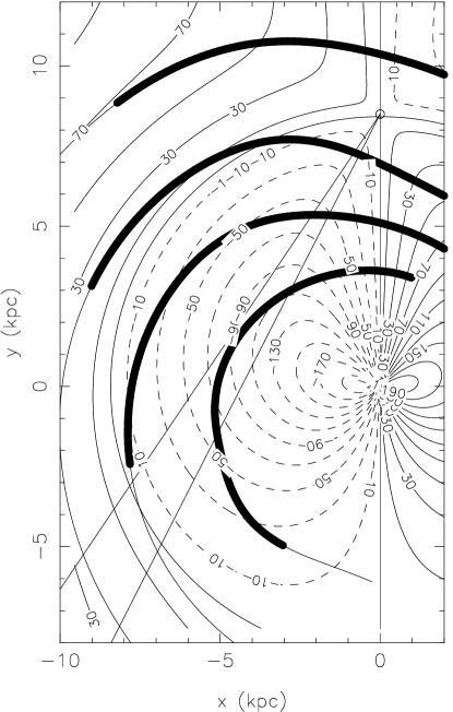
Figure 10: A face-on view of the Galaxy, with the longitude range of the SGPS test region indicated by two lines at longitudes 326°and 333°. The right panel has the radial velocities predicted from the rotation curve drawn as contours; the left panel shows some annular bins which are crossed by the lines of sight at the edges of the region. The annuli used for the averages shown on figure 9 are much narrower than those shown here, and there are many more of them. Both figures have the spiral arm model of Taylor and Cordes (1993) superposed. Common names for the spiral features are Norma (labelled “a”), Scutum-Crux (“b”), Sagitarius-Carina (“c”), and Perseus (“d”).

Figure 10 shows the geometry of the Galactic plane in the fourth quadrant (from McClure-Griffiths et al. 2001). The sun’s location is assumed to be at $(x,y)=(0,8.5)$, and we plot lines of sight at longitude 326°and 333°, the boundaries of the test region studied in this paper. Annuli are plotted with radii from 0.4 to 1.0 $R_{\odot}$, and the major spiral features from the model of Taylor and Cordes (1993) are reproduced. We see that the Norma spiral arm dominates the radial range 0.5 to 0.6 $R_{\odot}$ near the tangent point, the Scutum-Crux arm at the near distance dominates radii 0.6 to 0.7 $R_{\odot}$, and Sagitarius-Carina dominates at about 0.85 $R_{\odot}$. There is a gap in the range 0.7 to 0.85 which is between arms. This appears to be reflected in a dip in $\kappa$ at about 0.8 $R_{\odot}$ on figure 9. Even in this dip, and at all other radii in the inner Galaxy, the opacity is larger than its solar circle value of about 5 km s^-1 kpc^-1.

This narrow longitude range may not be representative of the entire inner galaxy, so we must wait for the full SGPS survey area to be studied before deciding conclusively that the opacity increases as we go to smaller Galactic radii. In the first quadrant, Garwood and Dickey (1989) found about the same result for the solar circle opacity, but smaller values for the inner galaxy. However, recently Kolpak et al. (2002) have made more extensive observations with the VLA in the first quadrant, and they find a trend similar to what we see on figure 9. The difference may be due to the small numbers of lines of sight sampled in the Garwood and Dickey study, which may have preferentially sampled the regions between the spiral arms, which appear here to show opacities of 5 km s^-1 kpc^-1 or less, in contrast to the arm regions which can have $<\kappa>>20$ km s^-1 kpc^-1.

If the increase in $<\kappa>$ by a factor of three to five with decreasing Galactic radius from the solar circle to the molecular ring region at about 0.5 $R_{\odot}$ is typical of the disk overall, we may ask whether it is due simply to an increase in the surface density of gas. The HI surface density as traced by 21-cm emission surveys does not show an increase with decreasing R_gal in this longitude range (Burton 1988, fig. 7.15), but the molecular gas does. The strong variation of $<\kappa>$ tells us that the cool atomic gas, in contrast to the warm neutral medium that dominates the $\lambda$21-cm emissivity, is much more abundant in the inner galaxy than at the solar circle. This underlines the role of the CNM clouds as an intermediate population between structures in the WNM and the much denser and colder molecular clouds.

The integrals of the emission spectra are given on table 1, columns 8 and 9 in units of 10²⁰ cm^-2. Column 8 gives the integral of the emission uncorrected for absorption, i.e.

$$N_{t}\ =\ C_{H}\ \int{T_{B}(v)\ dv}.$$ (4)

where we integrate over the full negative velocity range corresponding to the inner Galaxy. In column 9 we take the emission integral over the restricted velocity range $\Delta V$ corresponding to the absorption integral in column 7 (i.e. from zero to just short of the recombination line velocity). For this velocity range we can correct the values of emission for absorption to get a better estimate of the true column density assuming a one-phase medium (see next section). That correction is given by

$$N_{c}\ =\ C_{H}\ \int_{\Delta V}{T_{B}(v)\ \frac{\tau}{1\ -\ e^{-\tau}}\ dv}.$$ (5)

The effect of this correction is to increase the column density by a factor that is typically between one and two. Values of the ratio $f_{c}\ \equiv\ \frac{N_{c}}{N_{t}}$ for the same range of integration, $\Delta V$ are given on table 1, column 10. These correction factors show typical values of 1.4 to 1.6, which is in agreement with similar correction factors found by Dickey and Benson (1982). Note that the $N_{t}$ values on Table 1, column 8 are typically larger than $N_{c}$ on column 9 because the range of integration is broader for the former than for the latter, the full inner Galaxy range for the former, and only to the recombination line velocity for the latter.

Finally we can combine the velocity integrals of the emission and absorption to get a velocity averaged spin temperature,

$$\left<T_{sp}\right>\ =\ \frac{N_{t}}{EW\ C_{H}}$$ (6)

which is the nominal value of the spin temperature needed to give the emission and absorption integrals if the gas were at a single temperature. This is given on table 1, column 11 for the velocity range corresponding to columns 7 and 9. Comparison of the emission and absorption spectra channel-by-channel shows that this value is far from realistic, even under the “one-phase” assumption.

4 How to Combine the Emission and Absorption Spectra to find the Diffuse Cloud Temperatures

Methods for combining the emission and absorption spectra to find the distribution of spin temperatures in the interstellar HI can get complicated. The complications arise from blending of gas at different temperatures in the same spectral channel. Any line of sight at low Galactic latitudes will contain a mixture of several cool clouds which appear as Gaussian line components in the absorption spectrum, plus warm gas which is hardly visible in the absorption spectrum, but which contributes the bulk of the emission. The challenge is to combine the absorption and emission spectra in a way which separates these two thermal phases, giving an estimate of the temperature of the cool gas without the bias introduced by the warm gas emission. In this section we discuss and compare several mathematical techniques for this.

4.1 Method 1. The One-Phase Model

The simplest way to combine the emission and absorption spectra is to ignore the blending and compute the excitation temperature for each velocity channel naively assuming all the gas at a given velocity is at the same temperature. This gives the simple formula:

$$T_{sp}(v)\ \ =\ \ \frac{T_{B}(v)}{1\ -\ e^{-\tau(v)}}$$ (7)

where $T_{B}$ is the brightness temperature of the emission in velocity channel $v$, and $\tau(v)$ is the optical depth of the absorption in the corresponding velocity channel. This gives the harmonic mean of the temperatures of the various neutral atomic regions which contribute to that velocity channel, i.e.

$$T_{sp}\ \ =\ \ \frac{\sum_{i}{N_{i}}}{\sum_{i}{\left(\frac{N_{i}}{T_{i}}\right)}}$$ (8)

where $i$ is an index for the different regions on the line of sight contributing, each with column density $N_{i}$ and excitation temperature $T_{i}$. The distribution of $T_{sp}$ vs. number of channels for the nine sources with $T_{c}>$30K is given on figure 11. We must assume that the temperatures resulting from equation 7 shown on figure 11 are strongly biased to higher values than the true cool HI temperature due to blending with the warm gas.

Figure 11: Histogram of the temperatures derived from the naive, one phase model ($T_{sp}$, eq. 7). The weighting is simply by number of channels, which roughly corresponds to weighting by volume rather than by mass.

4.2 Gaussian Fitting to the Absorption or to the Optical Depth

Improved estimates of the cool phase temperature are based on the shapes of the features in the emission and absorption spectra. A simple approach is to fit the absorption spectrum with a number of Gaussian components. Low latitude $\lambda$21-cm emission spectra do not generally look like the sum of distinct Gaussian components, but absorption spectra do, so this is a reasonable approach. When the Gaussian components blend together the best fit parameters become ambiguous, and for a complicated, low latitude spectrum even the number of Gaussian components needed is not clear. Thus there is no unique solution to the Gaussian fitting problem.

The fitted parameters are obtained using an interactive program based on the Levenberg-Marquardt method of non-linear chi-squared minization (Press et al., 1992). The numbered boxes above the spectra on figures 2-8 indicate the velocity ranges dominated by the different line components (given on Table 2, columns 6 and 7). Weaker components may be hidden below the stronger ones in these velocity ranges. Our detection limit for absorption features is thus a function of velocity, and is generally higher than that set by the noise. Note that these boxes do not represent velocity ranges over which the fitting is performed. In cases where several line components are blended we perform the fitting of all Gaussian parameters simultaneously over the full velocity range covered by all components, plus some baseline on either side.

For deep absorption lines such as those found at low latitudes, it is preferable on physical grounds to fit the absorption spectrum with a sum of functions which are Gaussian in the optical depth, $\tau$, rather than in the observed absorption, $e^{-\tau}$. We could do this by fitting Gaussians to the log of the observed $e^{-\tau}$ spectrum, but this amplifies the effect of the noise for the deeper lines; for a deep line with noise we can get $(1-e^{-\tau})>1$ which causes the log function to diverge. It is better to do the fitting using for the model a sum of functions of the form

$$(1\ -\ e^{-\tau(v)})_{model}\ =\ 1\ -\ e^{-\sum_{i}{\ \left[\tau_{0,i}\ e^{-\frac{(v-v_{0,i})^{2}}{2\sigma_{i}^{2}}}\right]}}$$ (9)

where the parameters $\tau_{0,i}$, $v_{0,i}$, and $\sigma_{i}$ for each line component $i$ are varied to minimize $\chi^{2}$ in the usual way (see table 2, columns 3-5). In spite of the double exponential this is no more difficult to fit to the data than a sum of ordinary Gaussians, and it provides a better match to the flat tops seen on the deeper lines. More importantly, the values of $\tau_{0,i}$ are significantly larger than the depths of the corresponding Gaussian fits, because of saturation. Thus the derived column densities for the cool gas are larger, often by a factor of two or more, than what would be obtained from simple Gaussian fits. The fitted parameters are obtained using an interactive program based on the Levenberg-Marquardt method of non-linear chi-squared minization (Press et al., 1992). The numbered boxes above the spectra on figures 2-8 indicate the velocity ranges dominated by the different line components (given on Table 2, columns 6 and 7). Weaker components may be hidden below the stronger ones in these velocity ranges. Our detection limit for absorption features is thus a function of velocity, and is generally higher than that set by the noise. Note that these boxes do not represent velocity ranges over which the fitting is performed. In cases where several line components are blended we perform the fitting of all Gaussian parameters simultaneously over the full velocity range covered by all components, plus some baseline on either side.

We cannot estimate the cool phase temperature directly from the widths of the Gaussians, however they are fitted, because turbulence and random motions on all scales have the effect of widening the line significantly beyond the thermal width given by the Maxwellian distribution of atomic velocities. So we need another approach to combine the emission and absorption spectra to get estimates for the temperatures of the cool phase gas and undo the blending of equation 8. The next simplest thing to do after the one-phase assumption of equation 7 is to assume the HI comes in two phases.

4.3 Method 2. Two Phase Linear Least-Squares Fitting

The two phase assumption attributes all the absorption to the cool clouds, while the emission spectrum includes the cloud emission plus emission from a warmer medium which is necessarily more broadly distributed in velocity. No assumption is made here about the spatial distribution of either phase, but the fact that optical depth spectra can be fitted by a sum of Gaussians suggests that the cool gas is confined to discrete structures. The assumption of two phases means that the observed brightness temperature is given by

$$T_{obs}(v)\ \ =\ \ T_{w,f}\ +\ T_{w,b}\ e^{-\tau}\ +\ T_{cool}\ \left(1\ -\ e^{-\tau}\right)\ +\ T_{cont}\ e^{-\tau}$$ (10)

where the absorption comes from a cloud with temperature $T_{cool}$ and optical depth $\tau$, and the warm, optically thin gas is partly in front of the cloud, $T_{w,f}$, and partly behind it, $T_{w,b}$. The last term provides for the presence of continuum emission, $T_{cont}$, which is also behind the cloud, and hence is partially absorbed by it. Note that the contribution to the brightness temperature from the warm gas has nothing to do with its physical temperature; so long as it is optically thin its brightness temperature is proportional only to the column density, $N_{w}$, in the velocity channel width $\delta v$, as $T_{w}=\frac{N_{w}}{\delta v\ C_{H}}$.

When we subtract the continuum from the emission spectrum to obtain the line brightness temperature, $T_{B}(v)$, as a function of Doppler velocity, $v$, then the last two terms in equation 10 combine as

$$T_{B}(v)\ \ =\ \ T_{w,f}\ +\ T_{w,b}\ e^{-\tau}\ +\ \left(T_{cool}\ -\ T_{cont}\right)\ \left(1\ -\ e^{-\tau}\right)$$ (11)

This simplifies further if we consider the observed quantity $\left(1\ -\ e^{-\tau}\right)$ to be an independent variable that we rename $x$, so that

$$T_{B}(v)\ \ =\ \ T_{w,f}\ +\ T_{w,b}\left(1-x\right)\ +\ x\left(T_{cool}\ -\ T_{cont}\right)$$ (12)

Next we make an assumption that is supported by observations at high and intermediate latitudes that the warm gas is broadly distributed in velocity relative to the widths of the cool clouds. So over the velocity range of a single absorption line component we can approximate the warm gas contribution as a linear function of velocity, i.e. $T_{w,f}=a_{0}+a_{1}v$ and $T_{w,b}=b_{0}+b_{1}v$ or for the total

$$T_{w,f}\ +\ T_{w,b}\ =\ c_{0}\ +\ c_{1}v.$$ (13)

with $a_{0}$, $a_{1}$, $b_{0}$, $b_{1}$, $c_{0}$, and $c_{1}$ all constants. Then we have simply

$$T_{B}(v)\ \ =\ \ \left(c_{0}\ +\ c_{1}v\right)\left(1\ -\ \epsilon x\right)\ +\ c_{2}x$$ (14)

where $c_{2}$ is the cool cloud temperature reduced by the background continuum, $c_{2}=(T_{cool}-T_{cont})$ and $\epsilon\equiv\frac{T_{w,b}}{T_{w,f}+T_{w,b}}$ is the fraction of the warm gas which is behind the cloud ($0\leq\epsilon\leq 1$). Here we will assume $\epsilon$ is constant across the velocity width of each absorption line component, though in general it may be a function of velocity. Note that the continuum brightness, $T_{cont}$, is not the brightness temperature $T_{c}$ of the background source towards which we measure the absorption, but the diffuse continuum in the directions of the nearby pointings which give the interpolated emission spectrum.

Given the observed absorption and emission spectra, we can perform a simple linear least-squares fit to the data in order to determine the values of $c_{0}$, $c_{1}$, and $c_{2}$ in equation 14. The independent variables are $v$ and $x$, and the dependent variable, $T_{B}$, we will call $y$ for simplicity. The solution is obtained by minimizing the value of $\chi^{2}$ in the same way as for polynomial fitting, which leads to a matrix inversion problem where the elements of the matrix are moments of various combinations of $v$, $x$, and $y$. For example,

$$\overline{vxy}\ =\ \frac{1}{n}\ \sum_{i}\ v_{i}\cdot x_{i}\cdot y_{i}$$ (15)

where the sum is taken over all spectral channels, $i=$ 1 to $n$, covered by a distinct absorption feature (which presumably corresponds to a single cool phase temperature). The parameter $\epsilon$ is carried through all the calculations explicitly, so that results can be found for any selected value of $\epsilon$. The advantage of this approach, compared with the Gaussian fits discussed above, is that there is no ambiguity in the results; the unique solution is found directly with no iteration and no need for a “first guess” input by hand. The equations needed to find this best fit are given in the appendix.

Figure 12: Detailed analysis of the variation of brightness temperature vs. optical depth. The top left panel shows at the top the emission-absorption spectrum pair toward G326.65+0.59 as in figure 3. The upper portions of the other panels show the same two spectra, but blowing up the velocity ranges indicated by the numbered boxes. The emission spectrum has superposed the least squares fit, and below the residuals (data minus fit). The linear function, $T_{w}$, is also shown with the emission spectrum. The graphs just below the absorption spectra are plots of $T_{B}$ vs. $x\equiv\left(1-e^{-\tau}\right)$. The x’s on these plots show the individual channel values. The solid curve on the $T_{B}$ vs. $x$ plots shows the least squares fitted function of the form of equation 14. The coefficients of this function are indicated for each absorption feature sub-plot by the equation at the bottom.

Figure 13: Plots of the spectral features toward G326.65+0.59, continued from figure 12.

This fitting method is illustrated in figure 12-13, which show plots of the emission brightness temperature, $T_{B}$ against the observed absorption, $1-e^{-\tau}$. Different panels on figures 12-14 show separate line components toward G326.65+0.59, corresponding to the numbered boxes on the upper panel of figure 3. The solid curves show the fit results, and the symbols show the measured values in each velocity channel. In most cases the fits are quite good, considering that there are only three free parameters, and typically 10 to 15 independent pairs of measured quantities.

The approach taken here is very similar to that of Mebold et al. (1997) and Dickey et al. (2000) in their studies of the cool HI in the Magellanic Clouds. In those papers the fitting was done by hand by determining the “ridge-line” of each feature measured on the $T_{em}$ vs. $\tau$ plane like those in figures 12 and 13. That approach works best for simple spectra without blended absorption lines, as seen in the Magellanic Clouds and some high and intermediate latitude Galactic directions. At low latitudes the many overlapping absorption features make it difficult to draw the ridge lines by hand, so the fitting technique described in this section is needed. The results for unblended lines are very similar to those derived using the ridgeline method.

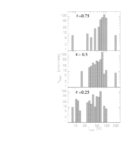
Figure 14: Histogram of $T_{cool}$. The histograms show the number of spectral channels at each temperature, derived using method 2 (linear least squares). Results for three values of $\epsilon$ are shown. The median values of $T_{cool}$ are 79 K, 65 K, and 51 K for $\epsilon$ = 0.75, 0.5, and 0.25, respectively.

The fitted values of $c_{0}$, $c_{1}$, and $c_{2}$ tell us both the temperature of the cool cloud ($T_{cool}=c_{2}+T_{cont}$) and the linear fit to the warm gas emission across the velocity range of the absorption line component (equation 13). These fit results are shown on table 2, columns 8 through 10. For this analysis we use only the five spectra toward continuum sources with T${}_{c,max}>$75 K, for which the rms errors in the absorption are less than 0.025. From these fits we can derive new histograms of cool gas temperatures. These are shown on figure 14, for three values of $\epsilon$=0.25, 0.50, and 0.75, which should bracket the true foreground - background distribution.

Figure 15: Detail of the linear least squares fitting results for G328.31+0.45. The upper spectrum (emission) shows both the data (x’s and the fitted emission profile, which are nearly indistinguishable, as well as the linear fits to the warm phase emission ($c_{0}+c_{1}v$). These piecewise linear fits are not continuous, either with each other or with the emission spectra on either side of the absorption features. This motivates the third method (non-linear least squares) for finding $T_{cool}$, which forces the warm phase models to be continuous.

Figure 14 shows simply the number of spectral channels covered by clouds with a given value of $T_{cool}$. This is not a mass weighted average, nor a volume average, but just the statistics of clouds sampled on the small number of lines of sight toward the five strongest continuum sources. Since the sample is small, and groups of channels come out with the same cloud temperature, the histograms have gaps at the lower temperatures, which are certainly unrealistic. These histograms must be considered merely representative of the distribution of HI cloud temperatures, with the general conclusion that most clouds have cool phase temperatures in the range 30 to 100 K, with occasional cooler values.

The parameter $\epsilon$ is undetermined for any given cloud. In general we may expect roughly half of the warm-phase gas to be in front of the absorbing cloud (at a given velocity) and half behind, which means $\epsilon\simeq 0.5$ is a good guess. The lower panel, which shows the result from setting $\epsilon=0.25$ for all clouds, certainly underestimates the temperatures of many clouds, since if only one quarter of the warm phase emission comes from behind the cloud, the cloud’s optical depth must be much higher, and hence its temperature cooler, then for $\epsilon$=0.5. Similarly, the upper panel, which assumes $\epsilon=0.75$ for all clouds, must overestimate the temperature of most clouds. An exception is the cloud centered on -5 km s^-1 toward G326.45+0.90. Fitting equation 14 to this results in a very cold temperature, 13 K assuming $\epsilon=0.75$, just 2 K if $\epsilon=0.5$, and -9 K for $\epsilon=0.25$. (In the middle and lower panels of figure 14 this cloud drops off the left edge of the plot.) The latter two are clearly unphysical, so in this case we may conclude that $\epsilon$ must be larger than $\sim 0.6$, and the cloud must be quite cold, strictly less than 25K, which is the value resulting from assuming $\epsilon=1$.

4.4 Method 3. Two Phase Non-Linear Least Squares Fitting

The linear least-squares fit technique described by equations 10-15 and in the appendix does a good job of matching the observed values of $T_{B}$ using the measured absorption values as the independent variable, but this technique ignores what we know about the warm gas emission at velocities on either side of the absorption line. Ideally the linear approximation to $T_{w}$ given by $c_{0}+c_{1}v$ should be continuous with the emission spectrum above and below the velocities covered by the absorption line, and in the case of multiple overlapping absorption lines, piecewise linear fits should be continuous between sequential velocity ranges. But this constraint is not incorporated into the fitting algebra, and typically it is not satisfied. An example is shown on figure 15, where the separate least squares fits toward G328.31+0.45 are plotted together. The discontinuities between successive linear approximations to $T_{w}$ show that we are still missing some information that could improve the model of the HI temperatures.

To force continuity in the $T_{w}$ model we have to return to a non-linear least-squares fitting technique, based again on the Levenberg-Marquardt method. This is a more complicated application, however, as we are now fitting a model to $T_{B}(v)$ using two independent variables, $v$ and $x\equiv(1-e^{-\tau(v)})$, and a set of parameters. The parameters are $c_{2}\equiv(T_{cool}-T_{cont})$ for each line component, and now instead of $c_{0}$ and $c_{1}$ to describe the warm gas emission for each velocity range, we have just one parameter for each contiguous box. For distinct velocity ranges (non-blended lines) the warm phase emission is fully determined by its values on either side of the absorption, and there is only one parameter to fit ($c_{2}$). For the case of overlapping lines, we can adjust the warm phase component arbitrarily at the boundary between the boxes, but in each box we stick to a linear interpolation for our estimate of the warm phase emission. Thus for blended absorption lines we are fitting both the cool phase temperature and the value of $T_{w}$ at each velocity edge where individual components overlap. The piecewise linear approximation to $T_{w}(v)$ is now fully specified by the values $T_{w}(v_{i})$, where the set of $v_{i}$’s are the boundaries of the velocity ranges represented by the boxes on figure 15. This forces the piecewise linear model $T_{w}$ to be continuous from one component to the next. If we further require that $T_{w}$ be continuous with $T_{B}$ on the first and last velocity edge, i.e. where the absorption drops below its detection threshold, then for a set of $n$ overlapping line components we have to fit just $n$ values of $c_{2}$ and $(n-1)$ values of $T_{w}(v_{i})$, where $i=2,...,n$ and $T_{w}(v_{1})$ and $T_{w}(v_{n+1})$ are fixed. Figure 16 shows the same spectral pair as in figure 15 (G328.32+0.45), but now fitted using method 3. The estimate of the warm phase contribution is much better behaved. The residuals of the fit to $T_{em}$ are shown at the bottom. Given that there are fewer than two free parameters to fit for each absorption component, the agreement between the data and the fit is impressive.

Figure 17 (lower panel) illustrates the distribution of cool phase temperatures resulting from this fitting for $\epsilon$=0.5, compared with a copy of the histogram for $\epsilon$=0.5 from figure 14. The third method of fitting changes the results slightly, mainly by reducing the higher values of $T_{cool}$ and so narrowing the peak near 70K. There is still a tail reaching to low temperatures, and the median value of $T_{cool}$ is hardly changed (67 K vs. 65 K from method 2).

Figure 16: Detail of the non-linear least squares fitting results for G328.31+0.45, as in figure 15. The piecewise linear fits for the warm phase emission are now much more reasonable. The data and the fitted values for the total emission are also shown, but almost indistinguishable. The residuals (data minus fit) are shown at the bottom.

For a single, isolated absorption component, the warm gas level is determined by a linear interpolation between the values of $T_{B}$ on the edges of the line, so there is only one parameter to fit, i.e. $c_{2}$, that determines the cool gas temperature. This effectively reduces to the method of interpolation used by Kalberla, Schwarz, and Goss (1985) in their study of the emission and absorption in the vicinity of 3C147, and by Mebold et al. (1982) in their study of several high and intermediate latitude regions. If we were to assume that the absorption and warm phase emission components could all be fitted by blended Gaussians then we could derive the cool phase temperature directly. This is the approach taken by Heiles and Troland (2002a,b) in their Arecibo survey of absorption and emission at intermediate latitudes. In appendix 2 we make a detailed comparison of their results with the results of our Method 2, and find that the differences are minor.

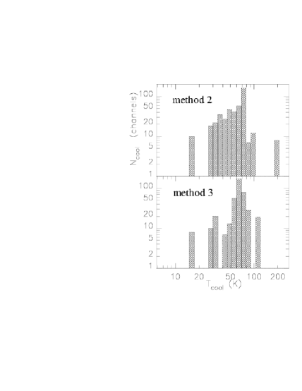
Figure 17: Comparison of the $T_{cool}$ distributions obtained with method 2 and method 3. Both histograms assume $\epsilon$=0.5. The upper histogram gives median $T_{cool}$ = 65 K, the lower histogram gives 67 K. Both are unweighted counts of spectral channels at each temperature, without regard to the total mass of gas in each channel.

5 Discussion

5.1 The Peak Brightness Temperature

The mean opacity, $<\kappa>$, derived in section 3 above plays a fundamental role in determining the radiative transfer of the 21-cm line across the Galactic plane. At low latitudes, cool clouds with optical depths of one or more are common enough that some, but not all, of the velocity range in a typical direction will be covered by optically thick gas. How likely this is depends on a contest between $<\kappa>$ and the velocity gradient, $\frac{dv}{ds}$, along the line of sight. These two quantities have the same units (km s^-1 kpc^-1), so we can make a dimensionless ratio, $\rho$, defined by

$$\rho\ \ \equiv\ \ \frac{\kappa}{\left|\frac{dv}{ds}\right|}$$ (16)

that depends on the local properties of the medium (the abundance of cool clouds) as well as on our particular vantage point (the longitude) and the shape of the rotation curve. In the extremely low velocity gradient case, as near longitudes 0°and 180°where $\frac{dv}{ds}\ \simeq\ 0$, this ratio $\rho$ is much greater than one, and the optical depth is high at all allowed velocities. In contrast, in the outer galaxy at a longitude where the velocity gradient is moderate, e.g. $\pm 90\deg$ for which $\left|\frac{dv}{ds}\right|\sim$ 10 km s^-1 along most of the line of sight, high optical depths are rare, since $\rho$ is less than one ($<\kappa>$ in the outer Galaxy is mostly below 5 km s^-1 kpc^-1). Since the absorbing gas is not smoothly distributed in space but is collected in discrete clouds with small filling factor, the spectra show occasional narrow features of significant optical depth even in regions where the mean optical depth is low. The ratio $\rho$ is useful for predicting optical depths averaged over velocity width $\Delta V$ broader than the linewidth of a single cloud, $\delta v\lesssim 5$ km s^-1.

Using the cool cloud temperature distribution, derived in section 4, together with $<\kappa>$, we can derive an approximate value for the peak brightness temperature of the Galactic 21-cm emission. It was noticed as early as the 1950’s in surveys of the Galactic plane that the 21-cm emission typically peaks at $T_{B}\sim$100 to 125 K, regardless of the direction or the velocity gradient. This is a curious fact, clearly seen in the spectra of the Weaver and Williams (1972) survey, for example. Since we know that the neutral hydrogen is spread fairly smoothly from the inner Galaxy to well outside the solar circle, we might expect the peak brightness temperature to correspond to low values of the velocity gradient, as it naturally would if most lines of sight were optically thin. On the other hand, we know that most of the HI is in the warm medium (roughly 75 %, Kulkarni 1983), so the peak brightness temperature does not simply correspond to the cloud temperature, $T_{cool}$, since the warm phase gas contributes most of the column density at any velocity. It is clear from emission-absorption spectrum pairs at low latitudes, like those in figures 2-8, that the peak brightness in emission does not always correspond to the velocities of high optical depths; on the contrary, deep absorption lines often correspond to dips in the emission brightness (i.e. HI self-absorption). It is a combination of the opacity, $<\kappa>$, the cloud temperature, $T_{cool}$, and the warm phase density, $n_{w}$, that determines the peak brightness temperature.

On a line of sight for which $\rho\gtrsim 1$, the 21-cm line is fairly optically thick, and the typical line of sight distance, $\Delta s$, needed to achieve average optical depth $\tau=1$ over some velocity width $\Delta V$ is

$$\Delta s\ =\ \frac{\Delta V}{<\kappa>}$$ (17)

since

$$<\kappa>\ \ =\ \ \frac{EW}{\Delta s}\ \ =\ \ \frac{\int_{\Delta V}{\tau\ dv}}{\Delta s}$$ (18)

If we assume that the warm phase gas has mean density $n_{w}$, then its column density over this line of sight interval is

$$N_{w}\ \ =\ \ n_{w}\ \Delta s\ \ =\ \ \frac{n_{w}\ \Delta V}{<\kappa>}$$ (19)

which, if there were no absorption, gives a velocity integral for the 21-cm line emission of

$$\int{T_{w,u}\ dv}\ \ =\ \ \frac{N_{w}}{C_{H}}$$ (20)

where the subscript $u$ indicates that this is the unabsorbed value, not what we actually see. Assuming once again that this warm phase emission is spread smoothly in velocity due to its broad natural line width ($\gtrsim 10$ km s^-1), we can take

$$\int_{\Delta V}{T_{w,u}\ dv}\ \ \simeq\ \ T_{w,u}\ \Delta V$$ (21)

which gives

$$T_{w,u}\ \ =\ \ \frac{N_{w}}{C_{H}\ \Delta V}\ =\ \frac{n_{w}}{C_{H}\ <\kappa>}.$$ (22)

As in equation 3, we can use $C_{H}=5.9\times 10^{-4}$ to get $T_{w,u}$ in K for $n_{w}$ in cm^-3 and $<\kappa>$ in km s^-1 kpc^-1. For a typical value of $n_{w}$=0.25 cm^-3 this gives $T_{w,u}\ \simeq\ \frac{400K}{<\kappa>}$, or about 80 K if $<\kappa>\simeq 5$ km s^-1 kpc^-1. Note that we have not had to assume a value of $\Delta V$ for this calculation, it can be anything between the typical absorption linewidth of $\lesssim$5 km s^-1 and the typical warm phase linewidth $\gtrsim$10 km s^-1.

The brightness temperature we expect from regions with $\rho\gtrsim 1$ is different from this, however, since $T_{w,u}$ is partially absorbed by the cool clouds before it gets to us, and the cool clouds themselves contribute some emission, given by $T_{cool}\ (1\ -\ e^{-\tau})$. If the warm phase gas is well mixed around and among the cool clouds, then its attenuated brightness temperature is given by

$$T_{w}\ \ =\ \ T_{w,u}\ \frac{1\ -\ e^{-\tau}}{\tau}$$ (23)

Adding on the emission from the cool cloud(s), $T_{cool}\ (\ 1\ -\ e^{-\tau})$, gives the total brightness temperature seen in emission

$$T_{B}\ \ =\ \ T_{cool}\ \left(1-e^{-\tau}\right)\ +\ \ T_{w,u}\ \frac{(1\ -\ e^{-\tau})}{\tau}.$$ (24)

For our assumed $\tau\simeq 1$ this gives $\sim$0.6 ($T_{cool}+T_{w,u}$), or about 0.6 (65K + 80K) = 87K.

In the alternative geometry assumed in section 4, where the warm phase gas is partly in front of the absorbing cloud and partly behind, we get

$$T_{B}\ \ =\ \ T_{cool}\ \left(1-e^{-\tau}\right)\ +\ \ T_{w,u}\ \left[1-\epsilon\left(1-e^{-\tau}\right)\right]$$ (25)

or, in the notation of equations 10 - 14,

$$T_{B}\ \ =\ \ T_{cool}\ x\ +\ T_{w,u}\ \left(\ 1\ -\ \epsilon\ x\right).$$ (26)

For $\epsilon$=0.5 and $x$=0.63 ($\tau$=1) this gives 102 K. In both cases the contributions from the warm and cool phases are about equal at about 50 K each. Going to higher optical depths does not change these numbers much. For $\tau\rightarrow\infty$ ($x\rightarrow 1$) equation 26 predicts $T_{B}\rightarrow 115$ K and in equation 24 the peak brightness actually decreases to approach $T_{cool}\simeq$ 65K. Of course the actual value of the peak brightness temperature will fluctuate around these values due to the relatively wide distribution of values of $T_{cool}$. The highest values we see presumably correspond to the warmer clouds ($T_{cool}\gtrsim 100$ K) and regions of relatively low $<\kappa>$, i.e. long path lengths between clouds.

In face-on disk galaxies the peak brightness temperature is much less dependent on the warm phase gas, since our lines of sight have path lengths of only a few hundred parsecs through the neutral hydrogen layer before hitting (or missing) a cloud. This explains why the brightness temperatures of the HI emission from nearby galaxies show such strong variation from place to place (Braun 1997). This ”high brightness network” probably traces the structure of the cloud phase of the medium, which may include a significant fraction of the warm gas with it. Payne, Salpeter and Terzian (1983), estimate that only about 30% of the total HI emission is from the widespread, “intercloud” medium, the rest is associated with the clouds, of which about half must be cool and the rest warm. Braun (1997) sees many examples of brightness temperatures above 150 K; the SMC shows a similarly high peak brightness temperature of 179 K (Stanimirovic et al., 1999). The implication of the high ends of the histograms in figures 14 and 17 is that there must be some clouds in the Milky Way with $T_{cool}$ as high as 150 K or more, although they are rare compared with the 50 to 100 K clouds. If we could get outside the Milky Way and look back, we might see those clouds unobscured by the cooler, more common clouds, so that seen from outside the Milky Way also may show brightness temperatures of 150 K or more. Braun (1997) also sees a radial variation in the brightness temperatures of the “high brightness network”, with brightness temperatures increasing with radius. This may be due to a radial variation of $T_{cool}$, but it could also be explained by a radial variation in $<\kappa>$ similar to what we find for the Milky Way in section 3; if $<\kappa>$ decreases with $R_{gal}$ then $T_{w,u}$ increases with $R_{gal}$ in equation 22, which makes the peak brightness temperatures increase.

The recognition that the peak brightness temperature of the 21-cm line at low latitudes results from a trade-off between absorption in the cool phase and emission from both warm and cool was first described by Baker and Burton (1975) in the context of radiative transfer models to fit the low latitude survey data then available. The role of the velocity gradient in the peak brightness temperature problem is discussed further by Burton (1993). The only innovation in the discussion above is to use the measured values of $<\kappa>$ together with the mean HI density to get a rough quantitative estimate for the value of the peak brightness temperature, rather than making a full cloudy medium model of the radiative transfer like that of Liszt (1983). The opacity function, $<\kappa(r)>$, incorporates the optical depth predictions of these models without making specific assumptions about clouds sizes or geometries.

5.2 HI Self-Absorption

Low latitude surveys of the Galactic 21-cm emission like the SGPS and the CGPS have turned up many examples of HI self-absorption (HISA, see Gibson et al., 2000, Minter et al. 2001, and Li and Goldsmith, 2002 for recent reviews). Earlier surveys with large single dish telescopes had shown that HISA is relatively common at low latitudes (Baker and Burton, 1979). It is often, but not always, associated with molecular line emission (Burton et al. 1978, Knapp 1974).

HISA is not true self-absorption, but absorption by cool foreground HI clouds of the background 21-cm line emission from warmer, more distant gas. Although temperature determinations for these HISA clouds are imprecise, typically they must be cooler than 40K, and sometimes as cold as 10 to 15K to fit the observations. Such cold HI may be inside molecular clouds, but this is not always the case. Although we do not yet have a complete catalog of such clouds, there are some large examples (Knee and Brunt 2001) which suggest that they may be common in the ISM. In this analysis there are some four clouds whose apparent temperatures are below 20 K, and several more between 20 and 40 K, depending on $\epsilon$. The most obvious is in box 4 toward G326.65+0.59 (-24 $<$ v $<$ -17 km s^-1 on figure 13). The effect of the cloud is to cause a deep dip in the emission spectrum at these velocities.

In principle, any cloud whose optical depth profile corresponds to a dip in the emission spectrum, rather than a peak, qualifies as HISA. In the notation of equation 14, this criterion amounts to

$$s\ \equiv\ c_{2}\ -\ \epsilon\ \left(c_{0}\ +\ c_{1}\right)\ <\ 0$$ (27)

so that the dependence of $T_{B}$ on $x$ has a negative coefficient. For the $\epsilon$=0.5 case, the median value of $s$ is -2.5; fully 67% of the lines have slope $s<$0. Thus HISA is in fact more common than the alternative, i.e. more than half of all HI clouds, defined as distinguishable features in the optical depth spectrum, correspond to dips rather than peaks in the emission spectrum. The HISA clouds which can be distinguished on the HI emission survey maps must be a relatively small subset of this population, those which are either particularly close or particularly cold, so that they stand out in their obscuring effect on the background emission.

At low latitudes and velocities corresponding to the inner galaxy, the HISA effect is amplified for clouds on the near side of the sub-central point due to unrelated emission from gas at the same velocity on the far side. Depending on the latitude, this should typically increase the expected value of $\epsilon$ from 0.5 to as high as 0.75. Using $\epsilon$=0.75 changes the median value of the slope $s$ above only slightly, from -2.5 to -2.3, but still more than half of the clouds (55%) show negative values of $s$.

6 Conclusions

HI spectra from low latitude surveys of the inner galaxy can only be understood in terms of radiative transfer in a partially absorbing medium. The gas is far from optically thin, and it is far from isothermal, so neither of these simplifications can be used to understand the brightness temperatures we see in emission. In this paper we study emission-absorption spectrum pairs to try to understand the relationship between the optical depth and the brightness temperature through various clouds along several lines of sight.

This paper concentrates on a few spectra in a relatively small area of the Galactic plane in the fourth quadrant. We hope that the techniques described here will be useful to analyze spectra toward many more continuum sources throughout the SGPS, and perhaps in other similar surveys as well. Since the sample is small, the results described here must be considered as only representative; more precise, quantitative measurements of the properties of the cool neutral medium will come from larger samples of spectra.

The three quantities that determine the characteristics of the emission spectra that we see in low latitude surveys are the warm phase HI density, $n_{w}$, the temperature of the cool clouds, $T_{cool}$, and the average density of the cool medium, which sets the value of $<\kappa>$. This paper discusses the last two, the first has been determined from earlier surveys with lower resolution (see reviews by Burton, 1988, Dickey and Lockman, 1990). With these three quantities in hand, we can understand the peak brightness of the HI emission, the fraction of atomic gas in the warm and cool phases, and the significance and abundance of HISA features.

The major findings here are:

• The mean opacity, $<\kappa>$, increases as we go inward through the Galactic disk, from about 5 km s^-1 kpc^-1 at the solar circle to as much as 25 km s^-1 kpc^-1 in the molecular ring. This result is in agreement with the finding of Kolpak et al. (2002) for the first quadrant, but different from the earlier result of Garwood and Dickey (1989).

• The temperature of the HI in the cool clouds, $T_{cool}$, is lower than what we would derive from a simple division of the emission by the absorption, $T_{sp}$. This agrees qualitatively (but not quantitatively) with results of fitting high and intermediate latitude emission-absorption spectrum pairs by Heiles and Troland (2002). The cloud temperatures derived here are similar but slightly higher than temperatures obtained for HI clouds in the SMC (Dickey et al. 2000) and in the LMC (Mebold et al. 1997) using a similar method. Though the median cloud temperature is around 65K, the distribution of $T_{cool}$ has a tail reaching to very cold values (well below 40 K).

• Putting together the values of $<\kappa>$ and $T_{cool}$ we can derive a rough prediction for the peak brightness temperature of the Galactic HI emission, that agrees with the $\sim$125K that is seen, independent of the velocity gradient, in single dish emission surveys.

• The slopes of the fitted curves in the $T_{em}$, (1-e^-τ) plane suggest that HISA is a very widespread phenomenon. The striking examples of HISA clouds that we notice in emission surveys are only the particularly cold or fortuitously placed cases.

Extending these techniques to the full survey area will indicate whether these conclusions apply to the inner galaxy as a whole, and also give a much better determination of the distribution of cool cloud temperatures.

Appendix A Least Squares Solution

The best fit values of $c_{0}$, $c_{1}$, and $c_{2}$ in equation (14) are given by linear combinations of moments of the form shown in equation (15). The derivation of these formulae is very similar to the problem of finding the coefficients of the best fit polynomial. Begin by defining nine combinations of the moments :

$$Y_{1}\ =\ \overline{y}\ -\ \epsilon\ \overline{xy}$$ (A1)

$$Y_{2}\ =\ \overline{vy}\ -\ \epsilon\ \overline{vxy}$$ (A2)

$$Y_{3}\ =\ \overline{xy}$$ (A3)

$$K_{1}\ =\ 1\ -\ 2\epsilon\ \overline{x}\ +\ \epsilon^{2}\ \overline{x^{2}}$$ (A4)

$$K_{2}\ =\ \overline{v}\ -\ 2\epsilon\ \overline{vx}\ +\ \epsilon^{2}\ \overline{v\ x^{2}}$$ (A5)

$$K_{3}\ =\ \overline{x}\ -\ \epsilon\ \overline{x^{2}}$$ (A6)

$$K_{4}\ =\ \overline{v^{2}}\ -\ 2\epsilon\ \overline{v^{2}\ x}\ +\ \epsilon^{2}\ \overline{v^{2}\ x^{2}}$$ (A7)

$$K_{5}\ =\ \overline{vx}\ -\ \epsilon\ \overline{v\ x^{2}}$$ (A8)

$$K_{6}\ =\ \overline{x^{2}}$$ (A9)

then combine these to make four mixed quantities :

$$H_{1}\ =\ \left(Y_{3}\ -\ \frac{Y_{1}\ K_{3}}{K_{1}}\right)\left(K_{4}\ -\ \frac{K_{2}^{2}}{K_{1}}\right)$$ (A10)

$$H_{2}\ =\ \left(Y_{2}\ -\ \frac{Y_{1}\ K_{2}}{K_{1}}\right)\left(K_{5}\ -\ \frac{K_{2}\ K_{3}}{K_{1}}\right)$$ (A11)

$$H_{3}\ =\ \left(K_{6}\ -\ \frac{K_{3}^{2}}{K_{1}}\right)\left(K_{4}\ -\ \frac{K_{2}^{2}}{K_{1}}\right)$$ (A12)

$$H_{4}\ =\ \left(K_{5}\ -\ \frac{K_{2}\ K_{3}}{K_{1}}\right)^{2}$$ (A13)

and finally combining these we get simply

$$c_{2}\ =\ \frac{H_{1}\ -\ H_{2}}{H_{3}\ -H_{4}}$$ (A14)

$$c_{1}\ =\ \frac{Y_{2}-\frac{K_{2}\ Y_{1}}{K_{1}}\ -\ c_{2}\ \left(K_{5}\ -\ \frac{K_{2}\ K_{3}}{K_{1}}\right)}{K_{4}\ -\ \frac{K_{2}^{2}}{K_{1}}}$$ (A15)

and

$$c_{0}\ =\ \frac{Y_{1}\ -\ K_{2}c_{1}\ -\ K_{3}c_{2}}{K_{1}}$$ (A16)

Appendix B Comparison with the Method of Heiles and Troland

Using the Arecibo telescope, Heiles and Troland (2002a, b) have recently carried out a monumental survey of emission and absorption in the 21-cm line toward some 75 bright continuum sources at high and intermediate Galactic latitudes. This survey is complementary to the low latitude surveys because it samples primarily gas within two kpc of the sun, but it samples this nearby gas very well, since the continuum sources are bright and even with the 3′ (FWHM) beam of the Arecibo dish the spatial resolution at the distance of the gas is typically less than one parsec. We have analysed their spectra using the method described in section 4.3 above, to find the distribution of cool phase temperatures shown on figure 18. Counting each cloud (absorption feature) equally gives median temperature 31 K for this distribution. Weighting by the number of velocity channels in each cloud raises this median temperature to 35 K.

Figure 18: Distribution of cool cloud temperatures, $T_{cool}$, for the absorption lines in the survey of Heiles and Troland (2002a). The median cool phase temperature is 31 K.

This result is somewhat cooler than the median temperature found by Heiles and Troland (48K), so it is worth looking in detail at the difference between their analysis and ours in a few pairs of spectra. Table 4 from Heiles and Troland (2002a) gives a comparison between their method and a simpler version of our technique, which they call the “slope method” (Mebold et al. 1997). For two sources they take $\epsilon\simeq 0.5$ on this table, 3C333 and PKS0428+20 (which they correctly identify by this name on their table 2). For 3C333 they measure 29 K for $T_{cool}$ from the slope method, and 25 K by fitting Gaussians, whereas we measure 26 K using method 2 of section 4.3 above. For PKS0428+20 they measure 41 K and 2 K from the slope method for the two dominant features centered at +3 and +10 km s^-1 respectively (figures 19 and 20), while we find 38 K and 27 K. From Gaussian fitting, Heiles and Troland find 29 K for the first and two blended components at 27 K and 34 K for the second. These differences are minor, and they probably result from the apportionment of the warm phase emission between the warm and cool components of Heiles and Troland’s Gaussian analysis.

Figure 19: Details of the fitting of the emission toward the lower velocity absorption component of PKS0428+20. Heiles and Troland find 29 K for the cool phase temperature, while we find 38 K.

Figure 20: Details of the fitting of the emission toward the higher velocity absorption component of PKS0428+20. Heiles and Troland decompose this into two Gaussians with temperatures 27 K and 34 K, while we find 27 K for the combination.

The analysis method used by Heiles and Troland is to first decompose the absorption spectrum into the sum of several Gaussians (three in the case of PKS0428+20), and then to decompose the emission spectrum into the sum of several more Gaussians (five in this case), of which the centers and widths of the first three are set by the values obtained from fitting the absorption. This technique accomplishes the all-important separation of the emission into warm and cool components, where the sum of the emission Gaussians that are not seen in the absorption correspond to $T_{w,f}\ +\ T_{w,b}$ in equation 13.

There is no ”right answer” to the problem of fitting multiple Gaussians, the result depends on the number of components and the first guesses for their parameter values. The linear least squares method has this advantage, that the solution for $T_{cool}$ and $T_{w}$ is unique given only an assumed value of $\epsilon$ and the velocity ranges to use for the fitting. At low latitudes, the approach of Heiles and Troland is not an option, since the emission spectra are so complicated that Gaussian fitting is hopeless. In the higher latitude directions studied in the Arecibo survey it is possible to decompose the emission as well as the absorption into a few Gaussians, and this gives more physical information about the gas than the simple two-phase approximation used in this paper. In general the contribution to the emission by the components that are seen in absorption is less than the contribution from those that are not seen in absorption, i.e. the WNM components; typically more than half of the emission integral (column density) comes from Gaussians that are not visible in absorption, and so must be warmer than 150 to 200 K. There is a good qualitative agreement on this result between this paper and those of Heiles and Troland, in spite of some minor disagreements on specific values of $T_{cool}$ given by the two methods.

All methods of analysis seem to agree on the result that the typical temperatures of absorbing clouds in the high and intermediate latitude sample observed from Arecibo are cooler than the inner galaxy clouds from the SGPS studied in this paper. This may reflect a real gradient in the cool phase temperature, either with Galactic radius, $R$, or with height above the plane, $z$. This may result from the different conditions inside cloud complexes, i.e. the larger environments containing cool atomic and molecular clouds and HII regions. The Arecibo sample contains HI clouds that are mostly not associated with H II region complexes, they are in a typical interstellar radiation field. If more of the HI in the inner galaxy is recent photodissociation product due to the greater abundance of hot stars as suggested by Allen (2001), then the typical cool phase temperature might be elevated, or there might be still more blending of warm, cool, and intermediate temperatures that could bias our results to higher values of $T_{cool}$. If further study of the SGPS data confirms that there is a trend toward lower cool phase temperatures in HI clouds with increasing $R$, then the corresponding decrease in $<\kappa>$ with $R$ suggests that the abundance of cool clouds is decreasing rapidly with increasing $R$.

References

- (1) Allen, R.J., 2001, in Gas and Galaxy Evolution, ASP Conference Proceedings, Vol. 240, eds. J. E. Hibbard, M. Rupen, and J. H. van Gorkom [San Francisco: Astronomical Society of the Pacific] p. 331.
- (2) Baker, P.L. and Burton, W.B. 1975, Ap. J., 198, 281.
- (3) Baker, P.L. and Burton, W.B., 1979, A. and A. Supp., 35, 129.
- (4) Braun, R. 1997, Ap. J. 484, 637.
- (5) Burton, W.B., 1988, in Galactic and Extragalactic Radio Astronomy, 2nd ed., eds. G.L. Verschuur and K. Kellerman, (New York : Springer-Verlag) p. 295.
- (6) Burton, W.B., 1991, in The Galactic Interstellar Medium, Saas-Fe Advanced Course 21, eds. P. Bartholdi and D. Pfenninger [Berlin: Springer-Verlag] section 2.3, pp. 20-22.
- (7) Burton, W.B., Liszt, H.S., and Baker, P.L., 1978, Ap. J. Lett. 219, 67.
- (8) Caswell, J.L., and Haynes, R.F., 1987, A. and A. 171, 261.
- (9) Clark, B.G., Radhakrishnan, V., and Wilson, R.W., 1962, /apj 135, 151.
- (10) Clark, B.G., 1965, Ap. J., 142, 1398.
- (11) Deshpande, A.A., 2000, MNRAS, 317, 199.
- (12) Dickey, J.M., Kulkarni, S.R., Heiles, C.E., and van Gorkom, J.H., 1983, Ap. J. Supp. 53, 591.
- (13) Dickey, J.M. and Lockman, F.J., 1990, Ann. Rev. Astron. Astrophys., 28, 215.
- (14) Dickey, J.M., Mebold, U., Stanimirovic̀, S., and Staveley-Smith, L. 2000 ApJ536, 756
- (15) Dickey, J.M., McClure-Griffiths, N.M., Stanimirovic, S., Gaensler, B.M., Green, A.J., 2001, Ap.J. 561, 264.
- (16) Faison, M.D., Goss, W.M., 2001, A.J. 121, 2706.
- (17) Fich, M., Blitz, L., and Stark, A.A., 1989, ApJ342, 272.
- (18) Field, G.B., 1958, Proceedings of the IRE, 46, 240.
- (19) Field, G.B., Goldsmith, D.W., and Habing, H.J., 1969, Ap. J. Lett. 155, L149.
- (20) Gaensler, B.M., Dickel, J.R., and Green, A.J., 2000, Ap. J. 542, 380.
- (21) Garwood, R.W. and Dickey, J.M., 1989, Ap. J., 338, 841.
- (22) Gibson, S.J., Taylor, A.R., Higgs, L.A., and Dewdney, P.E., 2000 ApJ540, 851
- (23) Goss, W.M., Radhakrishnan, V., Brooks, J.W., and Murray, J.D., 1972, Ap. J. Supp. 24, 123.
- (24) Hagen, J.P., Lilley, A.E., and McClain, E.F., 1955, Ap.J. 122, 361.
- (25) Heiles, C., 2000, Tetons 4: Galactic Structure, Stars, and the Interstellar Medium, ASP Conf. Ser. 231, ed C.E. Woodward, M.D. Bicay, and J.M. Shull (San Francisco: Astonomical Society of the Pacific), p. 294.
- (26) Heiles, C., 2001, ApJ551, 105
- (27) Heiles, C. and Troland, T.H., 2002, Ap. J. in press (astro-ph 0207104).
- (28) Hughes, M.P., Thompson, A.R., and Colvin, R.S., 1971, Ap. J. Supp., 23, 323.
- (29) Kalberla, P.M.W., Schwarz, U.J., and Goss, W.M., 1985, Astron. Astrophys. 144, 27.
- (30) Knapp, G.R. 1974 AJ79, 527
- (31) Knee, L.B.G., and Brunt, C.M., 2001, Nature, 412, 308.
- (32) Kolpak, M. A., Jackson, J.M., Bania, T.M., and Dickey, J.M., 2002, Ap. J. in press.
- (33) Kuchar, T.A. and Bania, T.M., 1990, Ap. J. 352, 192.
- (34) Kulkarni, S.R., 1983, Ph.D. Thesis, U.C. Berkeley.
- (35) Kulkarni, S.R. and Heiles, C., 1988, in Galactic and Extragalactic Radio Astronomy, 2nd ed., eds. G.L. Verschuur and K. Kellerman, (New York : Springer-Verlag) p. 95.
- (36) Li, D. and Goldsmith, P.F., 2002, ApJsubmitted.
- (37) Liszt, H.S., 1983, ApJ275, 163.
- (38) Liszt, H., 2001, A&A 371, 698.
- (39) Minter, A.H., Lockman, F.J., Langston, G.I., and Lockman, J.A., 2001, ApJ555, 868.
- (40) McClure-Griffiths, N.M., Dickey, J.M., Gaensler, B.M., Green, A.J., Haynes, R.F., Wieringa, M.H., 2000, A.J. 119, 2828.
- (41) McClure-Griffiths, N.M., Green, A.J., Dickey, J.M., Gaensler, B.M., Haynes, R.F., Wieringa, M.H., 2001, Ap.J. 551, 394.
- (42) Mebold, U., Winnberg, A., Kalberla, P.M.W., and Goss, W.M., 1982, A&A, 115, 223.
- (43) Mebold, U., Dusterberg, C., Dickey, J.M., Staveley-Smith, L., Kalberla, P., Muller, H., and Osterberg, J., 1997, Ap. J. Lett, 490, 65.
- (44) Payne, H.E., Salpeter, E.E., and Terzian, Y., 1983, Ap. J. 272, 540.
- (45) Press, W.H., Teukolsky, S.A., Vetterling, W.T., and Flannery, B.P., 1992, “Numerical Recipes in Fortran. The art of scientific computing” (Cambridge: University Press) 2nd ed., p.678.
- (46) Radhakrishnan, V., Murray, J.D., Lockhart, P., and Whittle, R.P.J., 1972a, Ap. J. Suppl. 24, 15.
- (47) Radhakrishnan, V., Goss, W.M., Murray, J.D., and Brooks, J.W., 1972b, Ap. J. Supp. 24, 99.
- (48) Radhakrishnan, V., Murray, J.D., Lockhaart, P., and Whittle, R.P.J., 1972c, Ap. J. Supp. 24, 15.
- (49) Spitzer, L. Jr., 1977, Physical Processes in the Interstellar Medium, (New York : John Wiley), chap. 3.
- (50) Stanimirovic, S., Staveley-Smith, L., Dickey, J.M., Sault, R.J., and Snowden, S.L., 1999, MNRAS 302, 417.
- (51) Strasser, S. et al. 2002 in preparation.
- (52) Taylor, A.R., et al. 2002 in preparation.
- (53) Taylor, J.H. and Cordes, J.M., 1993, Ap. J. 411, 674.
- (54) Weaver, H. and Williams, D.R.W., 1973, Astron. Astrophys. Suppl., 8, 1.
- (55)
- (56)