astro-ph/0211258

CERN–TH/2002-207

UMN–TH–2115/02

TPI–MINN–02/44

Updated Nucleosynthesis Constraints on Unstable Relic Particles

Richard H. Cyburt¹, John Ellis², Brian D. Fields³ and Keith A. Olive^4
1Department of Physics, University of Illinois, Urbana, IL 61801
²Theory Division, CERN, CH 1211 Geneva 23, Switzerland
³Department of Astronomy, University of Illinois, Urbana, IL 61801
⁴Theoretical Physics Institute, University of Minnesota, Minneapolis, MN 55455, USA

Abstract

We revisit the upper limits on the abundance of unstable massive relic particles provided by the success of Big-Bang Nucleosynthesis calculations. We use the cosmic microwave background data to constrain the baryon-to-photon ratio, and incorporate an extensively updated compilation of cross sections into a new calculation of the network of reactions induced by electromagnetic showers that create and destroy the light elements deuterium, ³He, ⁴He, ⁶Li and ⁷Li. We derive analytic approximations that complement and check the full numerical calculations. Considerations of the abundances of ⁴He and ⁶Li exclude exceptional regions of parameter space that would otherwise have been permitted by deuterium alone. We illustrate our results by applying them to massive gravitinos. If they weigh $\sim 100$ GeV, their primordial abundance should have been below about $10^{-13}$ of the total entropy. This would imply an upper limit on the reheating temperature of a few times $10^{7}$ GeV, which could be a potential difficulty for some models of inflation. We discuss possible ways of evading this problem.

CERN–TH/2002-207

October 2002

1 Introduction

Some of the most stringent constraints on unstable massive particles are provided by their effects on the abundances of the light nuclei produced primordially in the early Universe via Big-Bang Nucleosynthesis (BBN) [1]-[14]. Astrophysical determinations of the abundances of D, ⁴He and ⁷Li agree with those found in homogeneous BBN calculations, for a suitable range of the baryon-to-photon ratio $\eta$ [15, 16]. The decay products of massive unstable particles such as gravitinos would have produced electromagnetic and/or hadronic showers in the early Universe, which could have either destroyed or created these nuclei, perturbing this concordance. Maintaining the concordance provides important upper limits on the abundances of such massive unstable particles. The power of this argument has recently been increased by observations of the power spectrum of fluctuations in the cosmic microwave background (CMB) [17]. These now provide an independent determination of $\eta$ that is in rather good agreement with the value suggested by BBN calculations [18]-[22], reducing one of the principal uncertainties in the previous BBN limits on massive unstable particles.

This development has triggered us to re-evaluate these BBN constraints. We do so via a new calculation of the network of nuclear reactions induced by electromagnetic showers that create and destroy the light elements deuterium (D), ³He, ⁴He, ⁶Li and ⁷Li. We perform a coupled-channel analysis of the light-element abundances, which enables us to analyze the possible existence of isolated ‘islands’ of parameter space that are not minor perturbations of standard homogeneous BBN calculations. In carrying out this program, we also take the opportunity to improve previous theoretical treatments of some reactions in essential ways. We also derive analytic approximations to our results, which serve as a check of the numerics, and offer additional insight into the essential physics.

Considerations of the D abundance alone would have led to the apparent existence of finely-tuned ‘tails’ of parameter space that extend the region allowed by standard BBN calculations to rather larger abundances of unstable relic particles. In the past, these ‘tails’ were argued to be excluded on the basis of the combined D + ³He abundance. It is now widely considered that the complicated chemical and stellar history of ³He renders such an argument unsafe [23]. However, we show here that these tails are excluded robustly by the astrophysical abundance of ⁴He, and also conflict with the measured ⁶Li abundance. These other abundances also exclude a disconnected ‘channel’ of parameter space that would have been allowed by the D abundance alone. Overall, the most stringent upper limit on the possible abundance of an unstable massive relic particle $X$ with lifetime $\tau_{X}\mathrel{\hbox to0.0pt{\raise 2.15277pt\hbox{$>$}\hss}{\lower 2.15277pt\hbox{$\sim$}}}10^{2}$ s is provided by the ⁶Li abundance. For $\tau_{X}=10^{8}$ s, we find

$$M_{X}{n_{X}^{0}\over n_{\gamma}^{0}}\;<\;{5.0}\!\times\!10^{-12}~{}{\rm GeV},$$ (1)

with the upper limit from the ⁴He abundance being about two orders of magnitude less stringent.

As an illustrative application of this new analysis, we reconsider the allowed abundance of unstable gravitinos ${\tilde{G}}$ with masses up to about 10 TeV, which are expected to have lifetimes $\mathrel{\hbox to0.0pt{\raise 2.15277pt\hbox{$>$}\hss}{\lower 2.15277pt\hbox{$\sim$}}}10^{2}$ s. Using standard calculations of thermal gravitino production in the early Universe [24] - [32] , [8], the constraint (1) suggests a stringent upper limit on the reheating temperature $T_{R}$ of the Universe following inflation:

$$T_{R}\mathrel{\hbox to0.0pt{\raise 2.15277pt\hbox{$<$}\hss}{\lower 2.15277pt\hbox{$\sim$}}}10^{6}~{}{\rm GeV~{}~{}for}~{}M_{\tilde{G}}\sim 100~{}{\rm GeV}.$$ (2)

Such a stringent upper limit can be problematic for standard inflationary models [33], some of which predict higher $T_{R}\sim 10^{12}$ GeV. A low reheating temperature might also be problematic for some models of baryogenesis in which thermal production of baryon-number-violating particles is necessary, though not for others. The simplest leptogenesis scenarios [34] require the production of a right-handed neutrino state whose decays violate lepton number. However, even scenarios which require the thermal production of right-handed neutrinos can in fact accommodate very low reheat temperatures [35, 36], and non-thermal production of particles with masses less than the inflaton mass is possible for very low reheating temperatures [37]. Leptogenesis scenarios [38] of this type as well as those involving preheating [39] have been proposed .

Reheat temperatures higher than (2) would be allowed if $\tau_{\tilde{G}}\mathrel{\hbox to0.0pt{\raise 2.15277pt\hbox{$<$}\hss}{\lower 2.15277pt\hbox{$\sim$}}}10^{4}$ s, as might occur if $M_{\tilde{G}}\mathrel{\raise 1.29167pt\hbox{$>$\kern-7.5pt\lower 4.30554pt\hbox{$\sim$}}}3$ TeV and/or the gravitino has many available decay modes. Alternatively, one may consider the possibility of a very light gravitino that would be stable or metastable. However, in this case the upper limit (1) would apply to the next-to-lightest supersymmetric particle (NLSP). In conventional MSSM scenarios with a very light gravitino, this might be the lightest neutralino $\chi$. However, the relic $\chi$ abundance may also be calculated, and is likely to conflict with the upper limit (1).

This brief discussion serves to emphasize the importance of evaluating the cosmological upper limit on the possible primordial abundance of unstable relic particles, to which the bulk of this paper is devoted. In Section 2, we discuss the most relevant photodissociation and photoproduction processes and describe their implementation in a code to calculate the network of reactions creating and destroying light elements in the early Universe. A brief discussion of the observational constraints used is in Section 3. Analytical and numerical results for light-element abundances are presented in Section 4. Our main constraints on unstable particles are described in Section 5, where we compare and combine the upper limits obtained by considering different light nuclei. Finally, in Section 6 we discuss in more detail the implications of our results for cosmological gravitinos. Section 7 contains some comments on particles with longer (and shorter) lifetimes. In Appendix A, we compile and discuss the cross sections used in this analysis.

2 Photon Injection and Abundance Evolution

As an example of the constraints imposed on the abundance of a heavy metastable particle by observations of light elements, we consider the radiative decay of a massive particle (such as a gravitino) with lifetime $\mathrel{\raise 1.29167pt\hbox{$>$\kern-7.5pt\lower 4.30554pt\hbox{$\sim$}}}10^{4}$ s. The energetic decay photon initiates an electromagnetic shower, which in turn initiates a network of nuclear interactions. The decays of some unstable heavy particles also initiate hadronic showers, which would provide an additional set of constraints. These are typically important for shorter lifetimes, $\tau\mathrel{\hbox to0.0pt{\raise 2.15277pt\hbox{$<$}\hss}{\lower 2.15277pt\hbox{$\sim$}}}10^{2}$ s. However, we restrict our attention in this paper to the network of reactions induced by electromagnetic showers, and comment on very short (and very long) lifetimes in Section 7.

2.1 The Initial Degraded Photon Spectrum

At the epoch of interest to us here, $\tau_{X}\mathrel{\hbox to0.0pt{\raise 2.15277pt\hbox{$>$}\hss}{\lower 2.15277pt\hbox{$\sim$}}}10^{4}$ sec, the massive gravitino is very non-relativistic, and can be treated as if at rest with respect to the background. We assume that a gravitino of mass $M_{X}$ decays into a photon ($\gamma$) and a neutralino ($\chi$), each with their respective energies,

$$\!\!\!\!\!\!\!\!\!\!\!E_{\gamma}=\frac{M_{X}^{2}-m_{\chi}^{2}}{2M_{X}}\ {\rm and}\ E_{\chi}=\frac{M_{X}^{2}+m_{\chi}^{2}}{2M_{X}}.$$ (3)

In the limit $M_{X}\gg m_{\chi}$, the energies become almost equal: $E_{\gamma}\sim E_{\chi}\sim\frac{1}{2}M_{X}$.

The primary photon with injection energy $E_{0}$ interacts with the background plasma and creates an electromagnetic cascade. The most rapid interactions in this cascade are pair production $\gamma\gamma_{\rm bg}\rightarrow e^{+}e^{-}$ off of background photons, and inverse compton scattering. These processes rapidly redistribute the injected energy, and the nonthermal photon spectrum rapidly reaches a quasi-static equilibrium as discussed in [7, 9, 10]. The “zeroth generation” quasi-equilibrium photon energy spectrum is

$$\!\!\!\!\!\!\!\!\!\!\!p_{\gamma}(E_{\gamma})=\left\{\begin{array}[]{lll}K_{0}\left(\frac{E_{X}}{E_{\gamma}}\right)^{1.5}&\mbox{if $E_{\gamma}<E_{X}$}\\ K_{0}\left(\frac{E_{X}}{E_{\gamma}}\right)^{2.0}&\mbox{for $E_{X}<E_{\gamma}<E_{C}$}\\ 0&\mbox{otherwise}\end{array}\right\}$$ (4)

where the normalization constant $K_{0}$ is determined by demanding that the total energy be equal to the injected energy: $K_{0}=E_{0}/[E_{X}^{2}(2+\ln{(E_{C}/E_{X})})]$. This spectrum is the same as that used by Protheroe, Stanev, & Berezinksy [10] and Jedamzik [12], and also agrees with the result of a detailed numerical integration of the full Bolzmann equation by Kawasaki and Moroi [9] . It is a broken power law with a transition at $E_{\gamma}=E_{X}$ and a high-energy cutoff at $E_{\gamma}=E_{C}$. We adopt the same energy limits as Kawasaki and Moroi, namely $E_{X}=m_{e}^{2}/80T$ and $E_{C}=m_{e}^{2}/22T$. Physically, these scales arise due to the competition between photon degradation rates. The scales rise as the temperature drops, in which case there exist more high-energy photons to break up nuclei.

The zeroth-generation nonthermal photons then suffer additional interactions of Compton scattering, ordinary pair production off of nuclei, and $\gamma-\gamma$ scattering. These slower processes further degrade the photon specturm. The evolution of the resulting “first-generation” photons is governed by

$$\!\!\!\!\!\!\!\!\!\!\!\frac{d{\mathcal{N}}_{\gamma}}{dt}(E_{\gamma})=\frac{n_{X}}{\tau_{X}}p_{\gamma}(E_{\gamma})-{\mathcal{N}}_{\gamma}(E_{\gamma})\Gamma_{\gamma}(E_{\gamma}),$$ (5)

where $n_{X}=n_{X}^{0}(1+z)^{3}\exp{(-t/\tau_{X})}$ and $\tau_{X}$ are the decaying particle number density at redshift $z$ and mean lifetime, respectively. Also, ${\mathcal{N}}_{\gamma}$ is the photon energy spectrum, which is simply the product of the density of states ${\mathcal{D}}_{\gamma}$ and the occupation number fraction $f_{\gamma}$. Integrating ${\mathcal{N}}_{\gamma}$ over all energies yields the number density $n_{\gamma}^{\rm inj}$ of the injected photons. Further, $\Gamma_{\gamma}$ is the rate at which the photons are further degraded through further interactions with the background plasma. The key difference between $p_{\gamma}$ and ${\mathcal{N}}_{\gamma}$ is that the rates degrading photons directly after injection are much faster than the rates that further degrade photon energy determining ${\mathcal{N}}_{\gamma}$. We note that the effects due to the expansion of the universe on the photon spectrum are negligible because, during this epoch, electromagnetic interactions are much faster than the expansion rate.

The dominant photon degradation rates are those for double photon scattering, Compton scattering and pair production off nuclei. Because their high rates are fast compared to the cosmic expansion, the photon distribution reaches quasi-static equilibrium (QSE). This distribution is given by setting (5) equal to zero, yielding

$$\!\!\!\!\!\!\!\!\!\!\!{\mathcal{N}}_{\gamma}^{\rm QSE}(E_{\gamma})=\frac{n_{X}p_{\gamma}(E_{\gamma})}{\Gamma_{\gamma}(E_{\gamma})\tau_{X}}.$$ (6)

This QSE solution is the same as that derived in [9], where it is called $f_{\gamma}(\epsilon_{\gamma})$. The photon spectrum $p_{\gamma}$ can be determined easily from this equation, knowing that double-photon scattering dominates the high-energy region, whereas Compton scattering and pair production off nuclei dominate at lower energies. We recall that the redshift dependence of this QSE solution lies entirely in $n_{X}$, $p_{\gamma}$, and $\Gamma_{\gamma}$.

2.2 Photo-Destruction and -Production of Nuclei

The equations governing the production and destruction of nuclei are very similar to those for photons, being given by

$$\!\!\!\!\!\!\!\!\!\!\!\frac{d{\mathcal{N}}_{A}}{dt}(E_{A})=J_{A}(E_{A})-{\mathcal{N}}_{A}(E_{A})\Gamma_{A}(E_{A}),$$ (7)

where $J_{A}$ and $\Gamma_{A}$ are the source and sink rates of primary species $A$. The derivative, $d/dt$ takes into account the redshifting of energies and the dilution of particles due to the expansion of the universe. The source terms for the primary species are due to the photodissociation of background particles, and are defined by:

$$\!\!\!\!\!\!\!\!\!\!\!J_{A}(E_{A})=\sum_{T}n_{T}\int_{0}^{\infty}\!\!\!\!\!dE_{\gamma}{\mathcal{N}}_{\gamma}^{\rm QSE}(E_{\gamma})\,\sigma_{\gamma+T\rightarrow A}(E_{\gamma})\,\delta\left[{\mathcal{E}}_{A}^{T}(E_{\gamma})-E_{A}\right],$$ (8)

where ${\mathcal{E}}_{A}^{T}(E_{\gamma})$ is the energy of the $A^{\rm th}$ species produced by the photodissociation reaction $\gamma+T\rightarrow A$. The sinks are similarly defined by

$$\!\!\!\!\!\!\!\!\!\!\!\Gamma_{A}(E_{A})=\sum_{P}\int_{0}^{\infty}\!\!\!\!\!dE_{\gamma}{\mathcal{N}}_{\gamma}^{\rm QSE}(E_{\gamma})\,\sigma_{\gamma+A\rightarrow P}(E_{\gamma}).$$ (9)

Since we are interested in calculating total abundances of elements, it is necessary to integrate (7) over the energy $E_{A}$. The equation then becomes

$$\!\!\!\!\!\!\!\!\!\!\!\frac{dn_{A}}{dt}=\sum_{T}n_{T}\int_{0}^{\infty}\!\!\!\!\!dE_{\gamma}{\mathcal{N}}_{\gamma}^{\rm QSE}(E_{\gamma})\,\sigma_{\gamma+T\rightarrow A}(E_{\gamma})-n_{A}\sum_{P}\int_{0}^{\infty}\!\!\!\!\!dE_{\gamma}{\mathcal{N}}_{\gamma}^{\rm QSE}(E_{\gamma})\,\sigma_{\gamma+A\rightarrow P}(E_{\gamma}).$$ (10)

This removes the redshifting term, leaving only the dilution term in the derivative, $d/dt$. It is useful to use the mole fraction $Y_{i}\equiv n_{i}/n_{\rm B}$ of baryons in a particular nuclide, rather than the absolute abundance. This allows us to take out the expansion effects, yielding

$$\!\!\!\!\!\!\!\!\!\!\!\frac{dY_{A}}{dt}=\sum_{T}Y_{T}\int_{0}^{\infty}dE_{\gamma}{\mathcal{N}}_{\gamma}^{\rm QSE}(E_{\gamma})\,\sigma_{\gamma+T\rightarrow A}(E_{\gamma})-Y_{A}\sum_{P}\int_{0}^{\infty}\!\!\!\!\!dE_{\gamma}{\mathcal{N}}_{\gamma}^{\rm QSE}(E_{\gamma})\,\sigma_{\gamma+A\rightarrow P}(E_{\gamma}),$$ (11)

where $n_{B}$ is the baryon number density and $d/dt$ is an ordinary time derivative. It is also convenient to change from time differentiation to differentiation with respect to redshift, and also to extract the factor $n_{X}E_{0}/\tau_{X}$ out of ${\mathcal{N}}_{\gamma}^{\rm QSE}$. In this way, we obtain

$$\frac{dY_{A}}{dz} = -\frac{rM_{X}n_{\gamma}^{0}}{H_{r}\tau_{X}}\exp{\left(\frac{-1}{H_{r}\tau_{X}(1+z)^{2}}\right)}$$ (14)

$$\times\left[\sum_{T}Y_{T}\int_{0}^{\infty}\!\!\!\!\!dE_{\gamma}\left(\frac{\tau_{X}}{E_{0}n_{X}}{\mathcal{N}}_{\gamma}^{\rm QSE}(E_{\gamma})\right)\,\sigma_{\gamma+T\rightarrow A}(E_{\gamma})\right.$$

$$\left.-Y_{A}\sum_{P}\int_{0}^{\infty}\!\!\!\!\!dE_{\gamma}\left(\frac{\tau_{X}}{E_{0}n_{X}}{\mathcal{N}}_{\gamma}^{\rm QSE}(E_{\gamma})\right)\,\sigma_{\gamma+A\rightarrow P}(E_{\gamma})\right],$$

where we have used $E_{0}=\frac{1}{2}M_{X}$ (corresponding to two-body decay into a photon and a particle of negligible mass), and have defined $r\equiv n_{X}^{0}/n_{\gamma}^{0}$ and $H_{r}\equiv\sqrt{32\pi G\rho_{rad}^{0}/3}$. We should note that, with these terms pulled out, the integrals become functions only of redshift, and the dependence on the properties of the decaying particle has been removed. This formulation is very useful in making the numerical implementation fast and efficient.

Table 1: The relevant photo-dissociation reactions and their respective threshold energies are listed in the Table below, and their cross sections are listed in Appendix A.

Reaction	Threshold (Eγ,th)
d($\gamma$,n)p	2.2246 MeV
t($\gamma$,n)d	6.2572 MeV
t($\gamma$,np)n	8.4818 MeV
3He($\gamma$,p)d	5.4935 MeV
3He($\gamma$,np)p	7.7181 MeV
4He($\gamma$,p)t	19.8139 MeV
4He($\gamma$,n)3He	20.5776 MeV
4He($\gamma$,d)d	23.8465 MeV
4He($\gamma$,np)d	26.0711 MeV
6Li($\gamma$,np)4He	3.6989 MeV
6Li($\gamma$,X)3A	15.7947 MeV
7Li($\gamma$,t)4He	2.4670 MeV
7Li($\gamma$,n)6Li	7.2400 MeV
7Li($\gamma$,2np)4He	10.9489 MeV
7Be($\gamma$,3He)4He	1.5866 MeV
7Be($\gamma$,p)6Li	5.6058 MeV
7Be($\gamma$,2pn)4He	9.3047 MeV

2.3 Secondary Element Production

In the previous Section we discussed the production of light elements by the photo-dissociation of heavier elements. However, the initial photo-production/destruction of light nuclei is not necessarily the only process that happens before thermalization. The primary interactions produce non-thermal particles, which then interact with the background plasma, degrading their energy. However, they may still have enough energy to initiate further, secondary nuclear interactions.

We now modify the evolution of the primary particles described in the previous section to include energy-degrading interactions:

$$\!\!\!\!\!\!\!\!\!\!\!\frac{d{\mathcal{N}}_{A}}{dt}(E_{A})=J_{A}(E_{A})-{\mathcal{N}}_{A}(E_{A})\Gamma_{A}(E_{A})-\frac{\partial}{\partial E_{A}}\left[b_{A}(E_{A}){\mathcal{N}}_{A}(E_{A})\right],$$ (15)

where we have added the last term to include the energy degradation of the species $A$, where $b_{A}=-dE/dt$ is the rate of energy loss. This term appears as an energy gradient, conserving particle number in the absence of sources and sinks.

In most situations, the energy degradation rate is much faster than any sink, so that the sinks can be ignored. For unstable particles, if the lifetime of the particle is comparable to the stopping time of that species, then the $\Gamma_{A}$ term cannot be ignored. In general the interactions are fast enough to reach a quasi-static equilibrium, but the form of the solution is somewhat more complicated than the photon case:

$$\!\!\!\!\!\!\!\!\!\!\!{\mathcal{N}}_{A}^{\rm QSE}(E_{A})=\frac{1}{b_{A}(E_{A})}\int_{E_{A}}^{\infty}\!\!\!\!\!dE_{A}^{{}^{\prime}}\exp{\left[-\int_{E_{A}}^{E_{A}^{{}^{\prime}}}dE_{A}^{{}^{\prime\prime}}\frac{\Gamma_{A}(E_{A}^{{}^{\prime\prime}})}{b_{A}(E_{A}^{{}^{\prime\prime}})}\right]}J_{A}(E_{A}^{{}^{\prime}}).$$ (16)

Substituting $J_{A}$ into this equation, we get

$$\!\!\!\!\!\!\!\!\!\!\!{\mathcal{N}}_{A}^{\rm QSE}(E_{A})=\frac{1}{b_{A}(E_{A})}\sum_{T}n_{T}\int_{{\mathcal{E}}_{A}^{-1}(E_{A})}^{\infty}\!\!\!\!\!dE_{\gamma}{\mathcal{N}}_{\gamma}(E_{\gamma})\sigma_{\gamma+T\rightarrow A}(E_{\gamma})\exp{\left[-\int_{E_{A}}^{{\mathcal{E}}_{A}(E_{\gamma})}dE_{A}^{{}^{\prime\prime}}\frac{\Gamma_{A}(E_{A}^{{}^{\prime\prime}})}{b_{A}(E_{A}^{{}^{\prime\prime}})}\right]}.$$ (17)

With this QSE solution in hand, we can determine the rate of secondary production of an element $S$:

$$\!\!\!\!\!\!\!\!\!\!\!\left.\frac{d{\mathcal{N}}_{S}}{dt}\right|_{\rm sec}\!\!\!\!\!\!\!(E_{S})=\sum_{T^{{}^{\prime}}}\int_{0}^{\infty}\!\!\!\!\!dE_{A}{\mathcal{N}}_{A}^{\rm QSE}(E_{A})\Gamma_{A+T^{{}^{\prime}}\rightarrow S}(E_{A})\delta\left[{\mathcal{E}}_{S}(E_{A})-E_{S}\right].$$ (18)

Integrating over $E_{S}$ yields:

$$\!\!\!\!\!\!\!\!\!\!\!\left.\frac{dn_{S}}{dt}\right|_{\rm sec}=\sum_{T^{{}^{\prime}}}n_{T^{{}^{\prime}}}\int_{0}^{\infty}\!\!\!\!\!dE_{A}{\mathcal{N}}_{A}^{\rm QSE}(E_{A})\sigma_{A+T^{{}^{\prime}}\rightarrow S}(E_{A})|v_{A}|.$$ (19)

Again, using the mole baryon fraction to remove expansion effects from the differential equation, we obtain

$$\!\!\!\!\!\!\!\!\!\!\!\left.\frac{dY_{S}}{dt}\right|_{\rm sec}=\sum_{T^{{}^{\prime}}}Y_{T^{{}^{\prime}}}\int_{0}^{\infty}\!\!\!\!\!dE_{A}{\mathcal{N}}_{A}^{\rm QSE}(E_{A})\sigma_{A+T^{{}^{\prime}}\rightarrow S}(E_{A})|v_{A}|.$$ (20)

Table 2: Relevant secondary reactions are listed below, in a format similar to Table 1.

Reaction	Threshold (Ep,th)
p(n,$\gamma$)d	0.0000 MeV
4He(t,n)6Li	8.3870 MeV
4He(3He,p)6Li	7.0477 MeV
4He(t,$\gamma$)7Li	0.0000 MeV
4He(3He,$\gamma$)7Be	0.0000 MeV

After some algebraic manipulation, we obtain the following evolution equation for secondary production:

$$\left.\frac{dY_{S}}{dz}\right|_{\rm sec}=-\frac{rM_{X}\eta(n_{\gamma}^{0})^{2}}{H_{r}\tau_{X}}(1+z)^{3}\exp{\left(\frac{-1}{H_{r}\tau_{X}(1+z)^{2}}\right)}\sum_{T,{T^{{}^{\prime}}}}Y_{T}Y_{T^{{}^{\prime}}}\int_{0}^{\infty}\!\!\!\!\!dE_{A}\frac{\sigma_{A+T^{{}^{\prime}}\rightarrow S}(E_{A})|v_{A}|}{b_{A}(E_{A})}$$

$$\times\int_{{\mathcal{E}}_{A}^{-1}(E_{A})}^{\infty}\!\!\!\!\!dE_{\gamma}\left(\frac{\tau_{X}}{E_{0}n_{X}}{\mathcal{N}}_{\gamma}^{\rm QSE}(E_{\gamma})\right)\sigma_{\gamma+T\rightarrow A}(E_{\gamma})\exp{\left[-\int_{E_{A}}^{{\mathcal{E}}_{A}(E_{\gamma})}dE_{A}^{{}^{\prime\prime}}\frac{\Gamma_{A}(E_{A}^{{}^{\prime\prime}})}{b_{A}(E_{A}^{{}^{\prime\prime}})}\right]},$$ (21)

where $\eta$ is the baryon-to-photon ratio: $\eta\equiv n_{\rm B}^{0}/n_{\gamma}^{0}$.

Table 2 lists the secondary reactions considered. Deuterium production does not occur within the lifetime range of interested to us, since the neutron decays before it has a chance to react with a proton to form deuterium, as pointed out in [7]. Also, we have verified that the secondary production of mass-7 elements is not significant, being small compared with that produced during BBN. The only significant secondary production is that of ⁶Li, as first shown in [12] and later in [13]. We show below that ⁶Li actually provides the strongest constraint for the lifetime range we are interested in. Note that the relevant threshold energies (Table 2) are those in which the nuclei are in the cosmic rest frame, and thus are computed in the fixed-target laboratory frame. Consequently, these are about a factor of two higher than the center-of-mass thresholds used in [12] and [13].

3 Observational Constraints

Before we discuss the results of our numerical analysis, we first discuss the current status of the observational determinations of the light-element abundances. The abundances subsequent to any photo-destruction/production must ultimately be related to these observations. Furthermore, our results are dependent on the assumed baryon-to-photon ratio, which may either be determined through the concordance of the BBN-produced abundances or through the analysis of the CMB spectrum of anisotropies. As noted above, there is relatively good agreement between the two.

3.1 Observed Light Element Abundances

Through painstaking observations of very different astronomical environments, primordial abundances can be inferred for D, ⁴He, and ⁷Li. In addition, ³He and ⁶Li have also been measured, and can provide important supplementary constraints. Here we summarize the data and our adopted limits: more detailed reviews appear in [15]. For all nuclides, accurate abundance measurements are challenging to obtain, due to systematic effects which arise from, e.g., an imperfect understanding of the astrophysical settings in which the observations are made, and from the process by which an abundance is inferred from an observed line strength.

Deuterium is measured in high-redshift QSO absorption line systems via its isotopic shift from hydrogen. In several absorbers of moderate column density (Lyman-limit systems), D has been observed in multiple Lyman transitions [42, 43]. Restricting our attention to the three most reliable regions [42], we find a weighted mean of

$$\!\!\!\!\!\!\!\!\!\!\!\left(\frac{\rm D}{\rm H}\right)_{p}=(2.9\pm 0.3)\times 10^{-5}.$$ (22)

We note, however, that the $\chi^{2}$ per degree of freedom is rather poor ( $\sim 3.4$), and that the unweighted dispersion of these data is $\sim 0.6\times 10^{-5}$. This already points to the dominance of systematic effects. Observation of D in systems with higher column density (damped systems) find lower D/H [44], at a level inconsistent with (22), further suggesting that systematic effects dominate the error budget [45]. If we used all five available observations, we would find D/H = $(2.6\pm 0.3)\times 10^{-5}$ with an even worse $\chi^{2}$ per degree of freedom ($\sim 4.3$) and an unweighted dispersion of 0.8. As an upper limit to D/H, we adopt the 2-$\sigma$ upper limit to the highest D/H value reliably observed, which is D/H = $(4.0\pm 0.65)\times 10^{-5}$, since we cannot definitively exclude the possibility that some D/H destruction has occurred in the other systems.

We also require a lower limit on the primordial D abundance. Since Galactic processes only destroy D, its present abundance in the interstellar medium[46], ${\rm D/H}=(1.5\pm 0.1)\times 10^{-5}$ provides an extreme lower limit on the primordial value, which is consistent with (22). Therefore, we adopt the limits

$$\!\!\!\!\!\!\!\!\!\!\!{1.3}\!\times\!10^{-5}<\left(\frac{\rm D}{\rm H}\right)_{p}<{5.3}\!\times\!10^{-5}.$$ (23)

This lower bound is quite conservative, in light of the fact that the existence of heavy elements confirms that stellar processing and thus D destruction has certainly occurred at some level.

Unlike D, ⁴He is made in stars, and thus co-produced with heavy elements. Hence the best sites for determining the primordial ⁴He abundance are in metal-poor regions of hot, ionized gas in nearby external galaxies (extragalactic HII regions). Helium indeed shows a linear correlation with metallicity in these systems, and the extrapolation to zero metallicity gives the primordial abundance (baryonic mass fraction) [47]

$$\!\!\!\!\!\!\!\!\!\!\!Y_{p}=0.238\pm 0.002\pm 0.005.$$ (24)

Here, the first error is statistical and reflects the large sample of systems, whilst the second error is systematic and dominates.

The systematic uncertainties in these observations have not been thoroughly explored to date [48]. In particular, there may be reason to suspect that the above primordial abundance will be increased due to effects such as underlying stellar absorption in the HII regions. We note that other analyses give similar results: $Y_{p}=0.244\pm 0.002\pm 0.005$ [49] and 0.239 $\pm 0.002$ [50]. For concreteness, we use the ⁴He abundance in (24) to obtain the range

$$\!\!\!\!\!\!\!\!\!\!\!0.227<Y_{p}<0.249,$$ (25)

taking the 2-$\sigma$ range with errors added in quadrature.

Helium-3 can be measured through its hyperfine emission in the radio band, and has been observed in HII regions in our Galaxy. These observations find [51] that there are no obvious trends in ³He with metallicity and location in the Galaxy, but rather a ³He ‘plateau’. There is, however, considerable scatter in the data by a factor $\sim 2$, some of which may be real. Unfortunately, the stellar and Galactic evolution of ³He is not yet sufficiently well understood to confirm whether ³He is increasing or decreasing from its primordial value [23]. Consequently, it is unclear whether the observed ³He ‘plateau’ (if it is such) represents an upper or lower limit to the primordial value. Therefore, we do not use ³He abundance as a constraint. If future observations of ³He could firmly establish the nature of its Galactic evolution, then ³He could be restored as a useful constraint on decaying particles, particularly in concert with D.

The primordial ⁷Li abundance comes from measurements in the atmospheres of primitive (Population II) stars in the stellar halo of our Galaxy. The ⁷Li/H abundance is found to be constant for stars with low metallicity, indicating a primordial component, and a recent determination gives

$$\!\!\!\!\!\!\!\!\!\!\!\left(\frac{\mbox{${}^{7}${\rm Li}}}{\rm H}\right)_{p}={(1.23\pm 0.06_{-0.32}^{+0.68})}\!\times\!10^{-10}\ ({\rm 95\%\ CL}),$$ (26)

where the small statistical error is overshadowed by systematic uncertainties [52]. The range (26) may, however, be underestimated, as a recent determination [53] uses a different procedure to determine stellar atmosphere parameters, and gives ${\mbox{${}^{7}${\rm Li}}/{\rm H}}_{p}=(2.19\pm 0.28)\times 10^{-10}$. At this stage, it is not possible to determine which method of analysis is more accurate, indicating the likelihood that the upper systematic uncertainty in (26) has been underestimated. Thus, in order to obtain a conservative bound from ⁷Li, we take the lower bound (once again combining the statistical and systematic errors in quadrature) from (26) and the upper bound from [53], giving

$$\!\!\!\!\!\!\!\!\!\!\!{9.0}\!\times\!10^{-11}<\left(\frac{\mbox{${}^{7}${\rm Li}}}{\rm H}\right)_{p}<{2.8}\!\times\!10^{-10}.$$ (27)

Finally, ⁶Li is also measured in halo stars, in which the ⁶Li/⁷Li ratio is inferred from the (thermally blended) isotopic line splitting. The lowest ⁶Li abudances comes from stars with primordial Li, which yield $\mbox{${}^{6}${\rm Li}}/\mbox{${}^{7}${\rm Li}}=0.05\pm 0.01$ [54]. The ⁶Li in these stars is not primordial, as it is produced by cosmic-ray interactions with the interstellar medium [55], predominantly $\alpha\alpha\rightarrow\mbox{${}^{6}${\rm Li}}+\cdots$. These same processes lead to the production of Be and B, which are observed in halo stars at levels consistent with ⁶Li cosmic-ray production. Since the observed ⁶Li abundances are consistent with being entirely Galactic in origin, we can use these to set an extreme upper limit on the primordial ⁶Li abundance. One complication enters, due to the smaller binding energy of ⁶Li relative to ⁷Li. This means that ⁶Li could in principle suffer depletion in stars due to nuclear burning, without a similar depletion of ⁷Li. However, once nuclear burning becomes effective, ⁶Li depletion factors become extrelemly large making such observations extremely unlikely [56]. It is therefore safe to use the 2-$\sigma$ upper bound on the ⁶Li/⁷Li ratio

$$\!\!\!\!\!\!\!\!\!\!\!\left(\frac{\mbox{${}^{6}${\rm Li}}}{\mbox{${}^{7}${\rm Li}}}\right)\mathrel{\raise 1.29167pt\hbox{$<$\kern-7.5pt\lower 4.30554pt\hbox{$\sim$}}}0.07.$$ (28)

Other depletion processes such as diffusion (included in the estimate of systematic uncertainties in (26)), would affect both ⁶Li and ⁷Li similarly and not their ratio. It is also useful to consider the upper bound on ⁶Li/H alone

$$\!\!\!\!\!\!\!\!\!\!\!\left(\frac{\mbox{${}^{6}${\rm Li}}}{\rm H}\right)_{p}\mathrel{\raise 1.29167pt\hbox{$<$\kern-7.5pt\lower 4.30554pt\hbox{$\sim$}}}2\times 10^{-11}.$$ (29)

3.2 Cosmic Microwave Background Anisotropy Measurements

Cosmic Microwave Background (CMB) anisotropy data are now reaching the precision where they can provide an accurate measure of the cosmic baryon content. Given a CMB measurement of $\eta$, one can use BBN to make definite predictions of the light element abundances, which can then be compared with the observations discussed above. This comparison constrains the effects of decaying particles more powerfully than if only the BBN calculations were available to constrain $\eta$.

Recent results from DASI [18] and CBI [19] indicate that $\Omega_{B}h^{2}=0.022^{+0.004}_{-0.003}$, while BOOMERanG-98 [20] gives $\Omega_{B}h^{2}=0.021^{+0.004}_{-0.003}$. These determinations are somewhat lower than the central values found by MAXIMA-1 [21]: $\Omega_{B}h^{2}=0.026^{+0.010}_{-0.006}$ and VSA [22]: $\Omega_{B}h^{2}=0.029\pm 0.009$. Taking a CMB value of

$$\!\!\!\!\!\!\!\!\!\!\!\Omega_{B}h^{2}=0.022\pm 0.003\qquad{\rm or}\qquad\eta_{\rm 10,cmb}=6.0\pm 0.8$$ (30)

at the 1-$\sigma$ level, we would predict the following light element abundances:

$$\mbox{${}^{4}${\rm He}}: 0.248\pm 0.001\ (68\%\ {\rm CL})$$ (31)

$${\rm D/H}\times 10^{5}: 2.7^{+0.9}_{-0.3}\ (68\%\ {\rm CL})$$ (32)

$${\rm\mbox{${}^{3}${\rm He}}/H}\times 10^{5}: 0.9\pm 0.1\ (68\%\ {\rm CL})$$ (33)

$${\rm\mbox{${}^{7}${\rm Li}}/H}\times 10^{10}: 3.4^{+1.5}_{-0.8}\ (68\%\ {\rm CL})$$ (34)

Note that these numbers are not outputs of BBN calculations corresponding to $\eta_{10}=6.0$, but rather are the peak values of a likelihood function found by convolving the results of the BBN Monte Carlo with an assumed Gaussian for the distribution of CMB $\eta$ values. For further details, see [16, 17]. With MAP data, the accuracy of $\eta_{\rm cmb}$ should be $10\%$ or better, which will give even tighter predictions on the light elements.

4 Model Results

We have implemented numerically the decaying-particle cascades discussed in Section 2. Using BBN light-element abundance predictions [16] as initial conditions, we calculate the final abundances for particular sets of baryon and dark matter parameters. The three free parameters are:

$$\!\!\!\!\!\!\!\!\!\!\!\zeta_{X}\equiv\frac{n_{X}^{0}}{n_{\gamma}^{0}}M_{X}=rM_{X}=2rE_{0},$$ (35)

$\tau_{X}$ and $\eta$.

4.1 Analytic Discussion

Some simple analytic approximations allow us to gain insight into the essential physics in our problem. As we will see, the following analytic treatment reproduces well the behavior of the light element abundance mountains and deserts in our parameter space.

The dependence on $\tau_{X}$ can be understood [11] in terms of the characteristic energy scales in the photon spectrum (4). Both the break $E_{X}$ and the cutoff $E_{C}$ scale as $E_{i}\propto 1/T$. Thus, in the ‘uniform decay’ approximation where all particles decay at $t=\tau_{X}$, the decay occurs at $T\sim 10^{-4}\,{\rm MeV}\,(\tau_{X}/10^{8}\,{\rm s})^{-1/2}$. Consequently, we have $E_{X}\sim 28\,{\rm MeV}\,(\tau_{X}/10^{8}\,{\rm s})^{1/2}$, and $E_{C}\sim 103\,{\rm MeV}\,(\tau_{X}/10^{8}\,{\rm s})^{1/2}$, and cutoffs thus increase with $\tau_{X}$. In other words, higher-energy photo-erosion processes can occur for longer lifetime values. Comparison with Table 1 shows that, as $\tau_{X}$ increases, first $E_{C}$ and then $E_{X}$ pass the threshold energy $E_{\rm th}$ for any given process, at which point the process becomes important. A reaction can turn on when $E_{C}\mathrel{\raise 1.29167pt\hbox{$>$\kern-7.5pt\lower 4.30554pt\hbox{$\sim$}}}E_{\rm th}$, which in the uniform decay approximation occurs when

$$\!\!\!\!\!\!\!\!\!\!\!\tau_{X}\mathrel{\raise 1.29167pt\hbox{$>$\kern-7.5pt\lower 4.30554pt\hbox{$\sim$}}}10^{6}\ {\rm s}\ \left(\frac{E_{\rm th}}{10\ {\rm MeV}}\right)^{2},$$ (36)

while for shorter $\tau_{X}$ the channel is closed. The reaction grows stronger when $E_{X}\mathrel{\raise 1.29167pt\hbox{$>$\kern-7.5pt\lower 4.30554pt\hbox{$\sim$}}}E_{\rm th}$, which occurs when

$$\!\!\!\!\!\!\!\!\!\!\!\tau_{X}\sim 10^{7}\ {\rm s}\ \left(\frac{E_{\rm th}}{10\ {\rm MeV}}\right)^{2}.$$ (37)

We can also understand the $\zeta_{X}$ dependence of photodestruction (and secondary production) analytically, as follows. In the limit of small $\zeta_{X}$, the decaying particle has no influence on the light-element abundances as predicted by primordial nucleosynthesis, predicting a universe made of mostly hydrogen and ⁴He, with small but significant amounts of D, ³He, and ⁷Li. Lithium-6 is not produced in significant quantities. Going beyond this trivial case we use a similar treatment as above, and employ the uniform decay approximation. To begin, as long as a reaction can proceed, a typical shower photon has energy

$$\!\!\!\!\!\!\!\!\!\!\!\langle E\rangle=56\ {\rm MeV}\left(\frac{E_{th}}{10\ {\rm MeV}}\right)^{\frac{1}{2}}\left(\frac{\tau_{X}}{10^{8}\ {\rm s}}\right)^{\frac{1}{4}},$$ (38)

so that the number of such photons per decay is $N_{\gamma}\sim E_{0}/\langle E\rangle$. Had the lower-energy piece of the power law been much steeper (i.e., with a power index $p>2$) we would have $\langle E\rangle\sim E_{th}$, and if it was much shallower (i.e., $p<1$) we would have $\langle E\rangle\sim E_{X}$. However, we lie in an interesting regime where $\langle E\rangle\sim(E_{th}/E_{X})^{P-1}E_{X}$, where $1<p<2$. Thus the nonthermal photon density is

$$\!\!\!\!\!\!\!\!\!\!\!n_{\gamma}^{\rm inj}=N_{\gamma}n_{X}=\frac{\zeta_{X}n_{\gamma}^{BG}}{2\langle E\rangle}.$$ (39)

These photons are thermalized at a rate per photon of $\Gamma_{\rm therm}\sim n_{e}\sigma_{\rm T}\sim n_{\rm B}\sigma_{\rm T}$. The rate per photon for the photodestruction of species $T$ to yield species $P$ is $\Gamma_{T\rightarrow P}\sim n_{T}\sigma_{T\rightarrow P}=f_{T\rightarrow P}Y_{T}\Gamma_{\rm therm}$, where $Y_{T}=n_{T}/n_{\rm B}$, and $f_{T\rightarrow P}=\sigma_{T\rightarrow P}/\sigma_{\rm T}$ is the relative strength of the cross section for photodestruction of $T$ into $P$, compared with the thermalization cross section, which we take as the Thompson cross section for this discussion. Consequently, the change in the number density of $A$ is the net production rate per volume $(\Gamma_{T\rightarrow A}-\Gamma_{A\rightarrow P})n_{\gamma}^{\rm inj}$ times the loss time $\Gamma_{\rm therm}^{-1}$, or

$$\!\!\!\!\!\!\!\!\!\!\!\delta n_{A}=n_{B}\delta Y_{A}\sim n_{\gamma}^{\rm inj}\frac{(\Gamma_{T\rightarrow A}-\Gamma_{A\rightarrow P})}{\Gamma_{\rm therm}}.$$ (40)

We see that the fractional change in an abundance is given by

$$\!\!\!\!\!\!\!\!\!\!\!\frac{\delta Y_{A}}{Y_{A}}\sim\frac{\zeta_{X}}{2\eta\langle E\rangle}\left(\frac{Y_{T}}{Y_{A}}f_{T\rightarrow A}-f_{A\rightarrow P}\right).$$ (41)

If we look at the two extremes when either production or destruction dominates, we can derive the behavior of $\zeta_{X}$, given that the fractional change in the abundance is $\sim 1/2$:

$$\zeta_{X}^{\rm prod} \sim {3.2}\!\times\!10^{-11}\ {\rm GeV}\left(5000\over\frac{Y_{T}}{Y_{A}}\right)\left({5.0}\!\times\!10^{-4}\over f_{T\rightarrow A}\right)\left(\eta_{10}\over 6\right)\left(E_{th}\over 20{\ \rm MeV}\right)^{\frac{1}{2}}\left(\tau_{X}\over 10^{8}{\ \rm s}\right)^{\frac{1}{4}},$$ (42)

$$\zeta_{X}^{\rm dest} \sim {6.3}\!\times\!10^{-8}\ {\rm GeV}\left({5.0}\!\times\!10^{-4}\over f_{A\rightarrow P}\right)\left(\eta_{10}\over 6\right)\left(E_{th}\over 2.224{\ \rm MeV}\right)^{\frac{1}{2}}\left(\tau_{X}\over 10^{8}{\ \rm s}\right)^{\frac{1}{4}},$$ (43)

where the numbers are those appropriate for D.

This same treatment can be extended to secondary production of light elements. Since ⁶Li is the only significant secondary production, this is the only example we consider here. In this case, only a fraction of the primary products have enough energy for this reaction to proceed, because of interactions with the background plasma. We estimate as follows the fraction that can react to form ⁶Li. Each prospective reactant is produced with initial energy ${\mathcal{E}}_{A}(\langle E\rangle)$, and the total amount of energy that can be lost between collisions is ${\mathcal{E}}_{loss}=b_{A}(\langle E\rangle)/n_{\rm B}\sigma_{T}|v_{A}|$. The fraction of reactants left is the ratio of these two energies, $N_{P}\sim{\mathcal{E}}_{A}(\langle E\rangle)/{\mathcal{E}}_{loss}\sim 0.001$. Thus the number density of these remaining non-thermal particles is

$$\!\!\!\!\!\!\!\!\!\!\!n_{P}^{\rm inj}=N_{P}\delta n_{A}\sim N_{P}\frac{\zeta_{X}Y_{T}n_{\rm B}}{2\eta\langle E\rangle}f_{T\rightarrow A}.$$ (44)

The rate per particle can be described in a similar way as before, where $\Gamma_{A\rightarrow S}=f_{A\rightarrow S}Y_{T^{{}^{\prime}}}\Gamma_{\rm therm}\beta$. Since these particles are non-relativistic, there is a factor $\beta=v/c$ in the interaction rate. We can thus determine the change in abundance of the secondary species:

$$\!\!\!\!\!\!\!\!\!\!\!\delta n_{S}\sim n_{\rm B}\delta Y_{S}\sim n_{P}^{\rm inj}\frac{\Gamma_{A\rightarrow S}}{\Gamma_{\rm therm}}.$$ (45)

The fractional change in the abundance is then given by

$$\!\!\!\!\!\!\!\!\!\!\!\frac{\delta Y_{S}}{Y_{S}}\sim N_{P}\frac{\zeta_{X}Y_{T}Y_{T^{{}^{\prime}}}}{2\eta\langle E\rangle Y_{S}}f_{T\rightarrow A}f_{A\rightarrow S}\beta.$$ (46)

Using parameters appropriate for ⁶Li and $\beta\sim 0.01$, we derive the value of $\zeta_{X}$ when secondary production becomes important:

$$\!\!\!\!\!\!\!\!\!\!\!\zeta_{X}^{sec}\sim{2.6}\!\times\!10^{-12}{\ \rm GeV}\left(\frac{{2.5}\!\times\!10^{11}}{\frac{Y_{T}Y_{T^{{}^{\prime}}}}{Y_{S}}}\right)\left(\frac{{5.0}\!\times\!10^{-4}}{f_{T\rightarrow A}}\right)\left(\frac{0.05}{f_{A\rightarrow S}}\right)\left(\frac{\eta_{10}}{6}\right)\left(\frac{E_{th}}{20{\ \rm MeV}}\right)^{\frac{1}{2}}\left(\frac{\tau_{X}}{10^{8}{\ \rm s}}\right)^{\frac{1}{4}}.$$ (47)

One should note that, at the high photon energies required to induce these tertiary reactions, double-photon scattering is comparable to the Compton scattering and nuclear pair-production mechanisms for photon energy-loss. This weakens the dependence of the reaction rates on the baryon density.

We now turn to the full numerical results, using these analytical estimates as a guide to interpretation.

4.2 Numerical Results

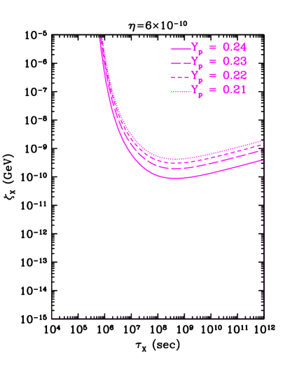
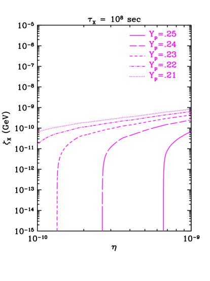
Figure 1: Contours of the ⁴He mass fraction $Y_{p}$ (a) in the $(\zeta_{X},\tau_{X})$ plane, for $\eta_{10}=6$, and (b) in the $(\zeta_{X},\eta)$ plane, for $\tau_{X}=10^{8}$ sec. See the text for discussion.

Our numerical results come from the integration of (14) and (2.3), using the input spectra of (4). We present our results by showing abundance contours in $\zeta_{X}-\tau_{X}$ space at fixed $\eta_{10}=6$, and in $\zeta_{X}-\eta$ space at fixed $\tau_{X}=10^{8}$ s. A key innovation of the present work is a detailed fitting of the energy dependence of the relevant cross sections. These are discussed in Appendix A, which also contains fitting formulae.

We begin our discussion with the most abundant compound nucleus, namely ⁴He. Since the other light elements are predicted by BBN to have abundances that are orders of magnitude smaller than ⁴He, no significant production of ⁴He can take place. Thus electromagnetic showers from decaying particles can only destroy ⁴He. These photodestruction processes have an energy threshold of $E_{\rm th}\sim 20$ MeV and so, from (36), we expect this process to become inefficient for $\tau_{X}\mathrel{\raise 1.29167pt\hbox{$<$\kern-7.5pt\lower 4.30554pt\hbox{$\sim$}}}4\times 10^{6}$ s, and to shut down completely when $\tau_{X}\mathrel{\raise 1.29167pt\hbox{$<$\kern-7.5pt\lower 4.30554pt\hbox{$\sim$}}}4\times 10^{5}$ seconds. Indeed, this is what is seen in Fig. 1(a), where we plot contours of $Y_{p}$ in the $(\zeta_{X},\tau_{X})$ plane for $\eta_{10}=6$, the value preferred by CMB analyses (30). For $\tau_{X}\mathrel{\raise 1.29167pt\hbox{$>$\kern-7.5pt\lower 4.30554pt\hbox{$\sim$}}}4\times 10^{6}$ s, the ⁴He destruction factor goes from a small perturbation to a large one as $\zeta_{X}$ grows from $10^{-10}$ to $10^{-9}$ GeV, until the region $\zeta_{X}\mathrel{\raise 1.29167pt\hbox{$>$\kern-7.5pt\lower 4.30554pt\hbox{$\sim$}}}10^{-8}$ GeV becomes a ⁴He ‘desert’. Over the region $\tau_{X}\sim 4\times 10^{5}\,{\rm s}-4\times 10^{6}\,{\rm s}$, ⁴He destruction becomes important only at increasingly high $\zeta_{X}$. This general behavior has an impact on all of the other light elements, as ⁴He is the only important source for them.

In Fig. 1(b), we again plot contours of Y_p, but now in the $(\zeta_{X},\eta)$ plane for $\tau_{X}=10^{8}$ s. We see the generic features mentioned above, that for low $\zeta_{X}$ ⁴He is at its BBN predicted value and for very large $\zeta_{X}$ it is destroyed. At large $\eta$, the non-thermal photons are more quickly thermalized, thus having less energy on average and making it more difficult to destroy nuclei. This linear rise is as predicted in (42).

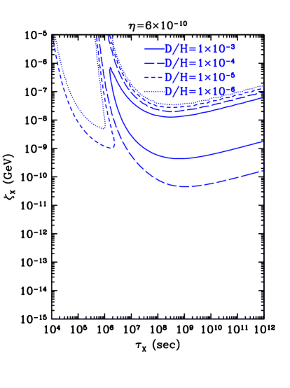
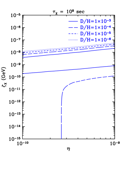
Figure 2: Deuterium abundance contours plotted as in Fig. 1.

Fig. 2 plots the corresponding contours of D/H. Several distinct regions are apparent. For all $\tau_{X}$, in the region $\zeta_{X}\mathrel{\raise 1.29167pt\hbox{$<$\kern-7.5pt\lower 4.30554pt\hbox{$\sim$}}}10^{-11}$ GeV, the decaying particles make only a small perturbation to the primordial value of D/H. For values of $\zeta_{X}\mathrel{\raise 1.29167pt\hbox{$>$\kern-7.5pt\lower 4.30554pt\hbox{$\sim$}}}10^{-11}$ GeV, the decaying particles can lead to significant perturbations to D/H, the sign and magnitude of which depend strongly on $\tau_{X}$. In the case of D, the important production processes are due to $\mbox{${}^{4}${\rm He}}+\gamma$: the other light elements have negligible abundances compared to ⁴He, and thus are unimportant as D sources. The D production channels have thresholds $E_{\rm th}\sim 25$ MeV, so we expect these process to become inefficient for $\tau_{X}\mathrel{\raise 1.29167pt\hbox{$<$\kern-7.5pt\lower 4.30554pt\hbox{$\sim$}}}5\times 10^{6}$ s. Furthermore, production is only efficient when ⁴He destruction is not large, i.e., when $\zeta_{X}\mathrel{\raise 1.29167pt\hbox{$<$\kern-7.5pt\lower 4.30554pt\hbox{$\sim$}}}10^{-9}$ GeV. Of course, D production can only occur when there is sufficient ⁴He destruction, so we expect significant production to occur only up to some maximum $\zeta_{X}$. For higher $\zeta_{X}$, photo-destruction becomes so dominant that any production yields are immediately broken up via further photo-destruction reactions, leaving a universe filled with only protons. Thus, as $\zeta_{X}$ increases, the D/H abundance rapidly declines, dropping to and then below its primordial abundance, to approach zero in a D ‘desert’. Thus, we expect D production only in a region bounded from above and below in $\zeta_{X}$, and to the left by $\tau_{X}\mathrel{\raise 1.29167pt\hbox{$<$\kern-7.5pt\lower 4.30554pt\hbox{$\sim$}}}4\times 10^{6}$ s. These expectations are met by the D/H ‘mountain’ in Fig. 2, which stretches between $\zeta_{X}=10^{-10}$ GeV to $\zeta_{X}=10^{-8}$ GeV.

For $\tau_{X}\mathrel{\raise 1.29167pt\hbox{$<$\kern-7.5pt\lower 4.30554pt\hbox{$\sim$}}}5\times 10^{6}$ s, D production from ⁴He does not occur. Since the photo-destruction processes $d(\gamma,n)p$ has a threshold of $E_{\rm th}=2.224$ MeV (the D binding energy), D destruction drops out at $\tau_{X}\mathrel{\raise 1.29167pt\hbox{$<$\kern-7.5pt\lower 4.30554pt\hbox{$\sim$}}}4\times 10^{3}$ s, as seen in Fig. 2. Finally, note that the competing processes of D production and destruction balance for some regions of parameter space, where D retains its primordial values. These are the ‘channels’ which separate the regions we have already discussed.

In Fig. 2(b), the contours of D/H are shown in the $(\zeta_{X},\eta)$ plane for $\tau_{X}=10^{8}$ s. Just like ⁴He, these D contours show the features sketched out in our analytic discussion. For low $\zeta_{X}$, D is at its BBN value. At intermediate values, we are climbing the photo-production mountain. At even higher values of $\zeta_{X}$, we enter the photo-erosion desert. Again the dependences on $\eta$ are entirely due to the photon energy-loss mechanism being more efficient at higher baryon density.

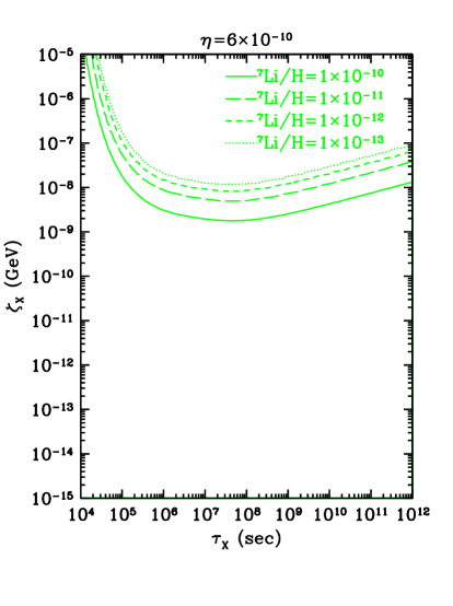
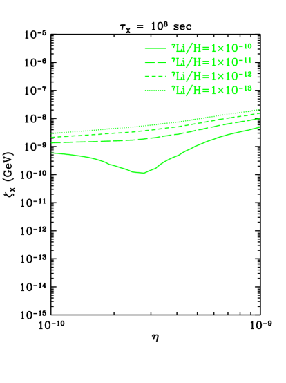
Figure 3: Contours of ⁷Li/H, plotted as in Fig. 1.

Results for ⁷Li/H are shown in Fig. 3. We see that the results are qualitatively similar to those for ⁴He, reflecting the fact that secondary ⁷Li production is negligible. Since ⁷Li is only destroyed, its weak binding compared to ⁴He leads to the wider expanse of the ⁷Li ‘desert’. As mentioned earlier, we considered the secondary production of ⁷Li, through the reactions ⁴He(t,$\gamma$)⁷Li and ⁴He(³He,$\gamma$)⁷Be. These reactions have no energy threshold, only a strong Coulomb barrier, so a priori they would seem important. However, the net production of ⁷Li through these reactions is small compared to its primordial value set by BBN. This is due to the small cross sections for mass-7 production.

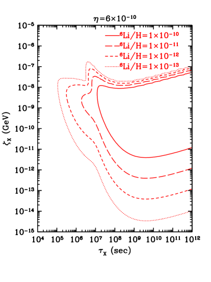
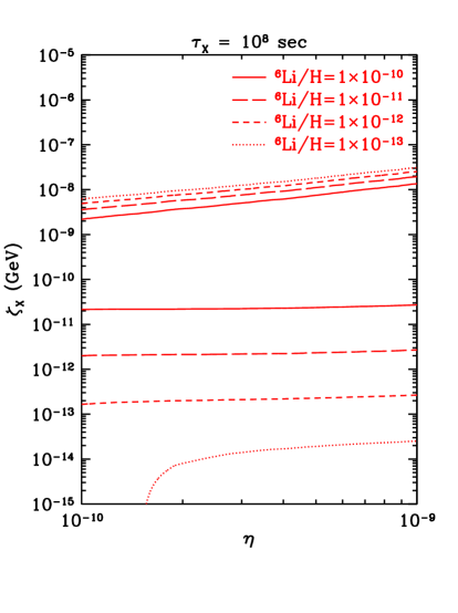
Figure 4: Contours of ⁶Li/H, plotted as in Fig. 1.

Unlike ⁷Li, standard BBN does not produce ⁶Li in any observable quantity, so any other production mechanism is important. The behavior of ⁶Li, seen in Fig. 4a, can be understood in terms of the ⁴He and ⁷Li dynamics, because these are the two ⁶Li sources. As with D, we see a roughly horizontal ‘mountain’ of ⁶Li production, which is bounded on the left by threshold effects. The dominant production channel is from secondary reactions, and thus is tied to the ⁴He destruction threshold. The secondary reactions ⁴He(t,n)⁶Li and ⁴He(³He,p)⁶Li, also have low energy resonances, further increasing their yields. The ⁶Li production from ⁷Li and ⁷Be, however, has lower thresholds, and thus becomes dominant for small lifetimes, $\tau_{X}\mathrel{\raise 1.29167pt\hbox{$<$\kern-7.5pt\lower 4.30554pt\hbox{$\sim$}}}10^{7}$ s. These channels are important where ⁷Li destruction is moderate but still sufficient to make significant amounts of ⁶Li, leading to a break in the slope of the ⁶Li curve at $\zeta_{X}\sim 10^{-11}$. The inclusion of two ⁶Li destruction channels leads to the ‘nose’ at $\zeta_{X}\sim 10^{-7}$ GeV and $\tau_{X}\sim 10^{7}$ s. This feature is absent in the ⁶Li plot in [13], since there only a single destruction channel was considered.

In Fig. 4b we see that the secondary production dominates the evolution of ⁶Li for quite low $\zeta_{X}$. Since the ⁶Li secondary-production cross sections have thresholds, the average initiating photon energy must be higher than in the standard photo-destruction process. In this higher-energy regime, double-photon scattering is comparable to the other photon energy-loss mechanisms. This reduces the dependence on the baryon density, effectively flattening out the contours in the $(\zeta_{X},\eta)$ plane where secondary production is important. At higher $\zeta_{X}$, photo-destruction of ⁶Li takes over, taking us to the ⁶Li desert.

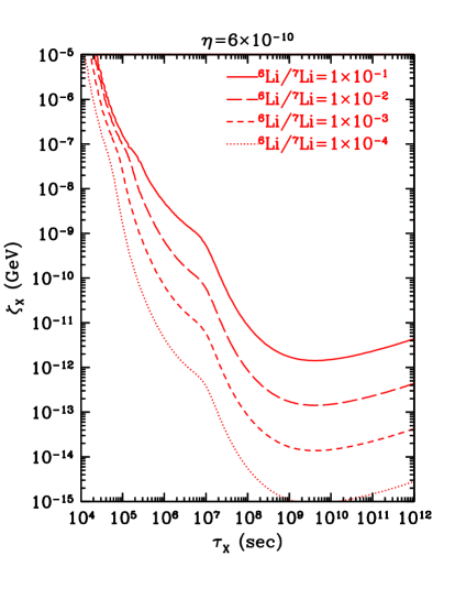
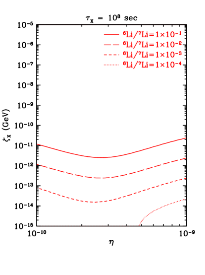
Figure 5: Contours of ⁶Li/⁷Li, plotted as in Fig. 1.

As noted in [11], the ⁶Li/⁷Li ratio offers additional constraints besides those provided by each nuclide separately. We plot ⁶Li/⁷Li contours in Fig. 5, where we see that these are smoother than the contours for ⁶Li alone. Because ⁶Li dissociation has a higher threshold than ⁷Li - see Table 1 - ⁶Li/⁷Li is large in the ‘desert’ region of high $\zeta_{X}$, though each individual abundance is quite small. For smaller $\zeta_{X}$, ⁶Li increases with $\zeta_{X}$, while ⁷Li either remains constant or decreases. The upshot is that ⁶Li/⁷Li grows with $\zeta_{X}$, as seen in Fig. 5.

Having described the physics that leads to the abundance patterns we have computed, we can now discuss how this physics allows the observed abundances to place constraints on decaying particles. To obtain these constraints, we combine this analysis with the observational data discussed previously.

5 Limits on Unstable Relic Particles

We now impose the observed light-element abundance constraints of Section 3.1 with the results of the previous section. We do this for each element individually, then combine the results to obtain the strongest constraints.

We remind the reader that light element constraints on decaying particles depend on $\eta$, but of course one cannot use the standard BBN limits on $\eta$ as part of ones limits. In the past, this difficulty has only been overcome by adopting limits on $\eta$ derived from non-nucleosynthetic arguments. These limits have, until recently, been rather weak, which has weakened the power of the light element constraints. This situation has now changed drastically. We recall that the CMB now imposes $\eta_{10}\simeq 6$ with rather small uncertainty. Thus, if we adopt the CMB results, we no longer must treat $\eta$ as weakly constrained by non-BBN arguments, strengthening the results we derive.

We quote limits for $\eta_{10}=6$, and emphasize results for $\tau_{X}=10^{8}$ s, which is roughly the lifetime for which the constraints are the strongest, and is also within the range of current interest for gravitino decays. Results at lower $\tau_{X}$ weaken rapidly, while the constraints at higher $\tau_{X}$ scale roughly as $\tau_{X}^{1/4}$, as in (42), (43) and (47).

Also, the current observational status of standard BBN comes into play. Namely, the present observational data on ⁴He and ⁷Li are in tension with those for D, the former preferring $\eta_{10}\sim 3$ and the latter $\eta_{10}\sim 6$. On the one hand, if standard BBN is correct and the tension is due to systematic errors, the result is that these errors weaken the constraints that one can place on decaying particles. On the other hand, if the observations were to improve to the point that the light-element disagreement can no longer be accommodated, this could herald new physics. In this case, decaying particles offer a way [11] of reconciling the abundances of the light elements, in which case one also derives estimates of the required $\zeta_{X}$ and $\tau_{X}$.

We turn first to the elements which are only destroyed, namely ⁴He and ⁷Li. The observed constraints on ⁴He (25) give

$$\!\!\!\!\!\!\!\!\!\!\!\zeta_{X}(\mbox{${}^{4}${\rm He}})<{2.5}\!\times\!10^{-10}\ {\rm GeV},$$ (48)

which is driven by the lower limit $Y_{p}>0.227$ that we adopted. The sharp drop of ⁴He with increasing $\zeta_{X}$ (i.e., the descent into the desert of Fig. 1) ensures that the constraint on $\zeta_{X}$ is insensitive to the precise $Y_{p}$ limit chosen. The situation is similar for ⁷Li, for which (27) give the weaker constraint

$$\!\!\!\!\!\!\!\!\!\!\!\zeta_{X}(\mbox{${}^{7}${\rm Li}})<{2}\!\times\!10^{-9}\ {\rm GeV}.$$ (49)

For deuterium, net production and net destruction are both possible. In terms of Fig. 2, this means that limits on D exclude the ridge in the D mountain, while allowing regions at higher and lower $\zeta_{X}$. In particular, the observed D abundances (22) allow the range ${2}\!\times\!10^{-8}\ {\rm GeV}\mathrel{\raise 1.29167pt\hbox{$<$\kern-7.5pt\lower 4.30554pt\hbox{$\sim$}}}\zeta_{X}\mathrel{\raise 1.29167pt\hbox{$<$\kern-7.5pt\lower 4.30554pt\hbox{$\sim$}}}{3}\!\times\!10^{-8}\ {\rm GeV}$, but the ⁴He and ⁷Li constraints are each able to exclude this regime. Consequently, the only remaining region is the low-$\zeta$ side of the mountain,

$$\!\!\!\!\!\!\!\!\!\!\!\zeta_{X}({\rm D})<{3}\!\times\!10^{-11}\ {\rm GeV}.$$ (50)

The since ⁶Li is not produced significantly in standard BBN, only production is important for low $\zeta_{X}$, while for higher $\zeta_{X}$ destruction dominates. Thus, the situation is similar to that of D: there is a ⁶Li mountain, with the observations allowing a narrow high-$\zeta_{X}$ region and a large low-$\zeta_{X}$ region. The ⁶Li/H abundance of (29) gives

$$\!\!\!\!\!\!\!\!\!\!\!\zeta_{X}(\mbox{${}^{6}${\rm Li}})<{5}\!\times\!10^{-12}\ {\rm GeV}$$ (51)

in addition to a higher region that is discordant with ⁴He and ⁷Li. The ⁶Li/⁷Li ratio (28) gives

$$\!\!\!\!\!\!\!\!\!\!\!\zeta_{X}(\mbox{${}^{6}${\rm Li}}/\mbox{${}^{7}${\rm Li}})<{7.0}\!\times\!10^{-12}\ {\rm GeV}.$$ (52)

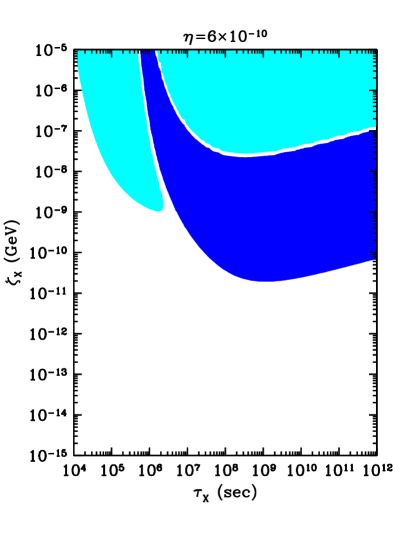
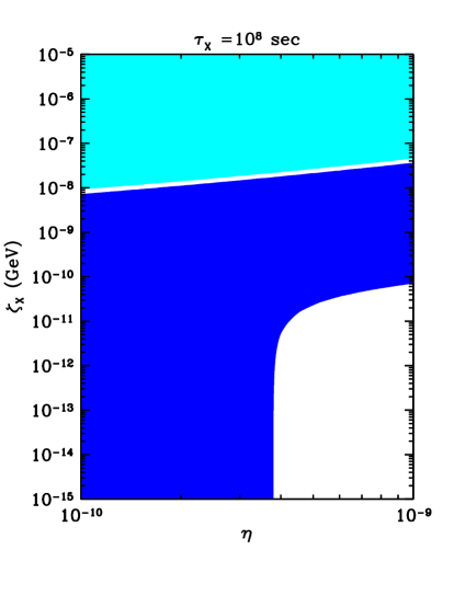
Figure 6: Exclusion limits based on deuterium are shown in (a) the $(\zeta_{X},\tau_{X})$ plane for $\eta_{10}=6$ (b) the $(\zeta_{X},\eta)$ plane for $\tau_{X}=10^{8}$ s. The dark (blue) shaded region corresponds to an overabundance of D/H, while the light (blue) shaded region corresponds to an underabundance of D/H.

Figure 6 summarizes our results for the constraints based on D/H in both the $(\zeta_{X},\tau_{X})$ plane (for $\eta_{10}=6$) and the $(\zeta_{X},\eta)$ plane for $\tau_{X}=10^{8}$ s. The dark (blue) shaded regions correspond to an overabundance of D/H, i.e. regions where there is net production of deuterium. The lighter (blue) shaded regions represent an underabundance of D/H or regions where there is net destruction of deuterium. Notice that the thin strips which are unshaded for which the D/H abundance is acceptable. These will be excluded when the constraints from the other light elements are included.

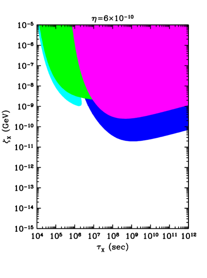
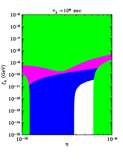
Figure 7: As in Figure 6, including the constraints from ⁴He - medium (pink) shading and ⁷Li - medium-light (green) shading.

In Figure 7, we include the constraints from ⁴He and ⁷Li. Here we superimpose the ⁴He constraint, shown as the medium shaded (pink) region. and the ⁷Li constraint, shown as the medium-light (green) shaded region, on the D/H constraints. We see that D, ⁴He, and ⁷Li alone, i.e., primordial species, impose a limit of

$$\!\!\!\!\!\!\!\!\!\!\!\zeta_{X}\mathrel{\raise 1.29167pt\hbox{$<$\kern-7.5pt\lower 4.30554pt\hbox{$\sim$}}}\zeta_{\rm max}={3.5}\!\times\!10^{-11}\ {\rm GeV},$$ (53)

which is dominated by the limits from D. We can do better if we include ⁶Li. Our limit ${\rm\mbox{${}^{6}${\rm Li}}/H}\mathrel{\raise 1.29167pt\hbox{$<$\kern-7.5pt\lower 4.30554pt\hbox{$\sim$}}}2\times 10^{-12}$ pushes the above constraint down to

$$\!\!\!\!\!\!\!\!\!\!\!\zeta_{X}\mathrel{\raise 1.29167pt\hbox{$<$\kern-7.5pt\lower 4.30554pt\hbox{$\sim$}}}\zeta_{\rm max}={5}\!\times\!10^{-12}\ {\rm GeV}$$ (54)

for $\tau_{X}=10^{8}$ s as seen in Figure 8 by the dark (red) shaded region. The constraint from the ⁶Li/⁷Li ratio is shown as the light (yellow) shaded region. Notice that it becomes the stronger constraint at $\eta<5.0$.

These constraints are subject to uncertainties in the ⁶Li limit, due both to the possible stellar depletion of ⁶Li and the known Galactic production of ⁶Li by cosmic rays. Our limit is intended conservatively to allow for both effects. Even so, we see the power of ⁶Li. We thus urge further observations of the Li isotopic ratio, as a firmer understanding of this nuclide could further strengthen the constraint we have derived.

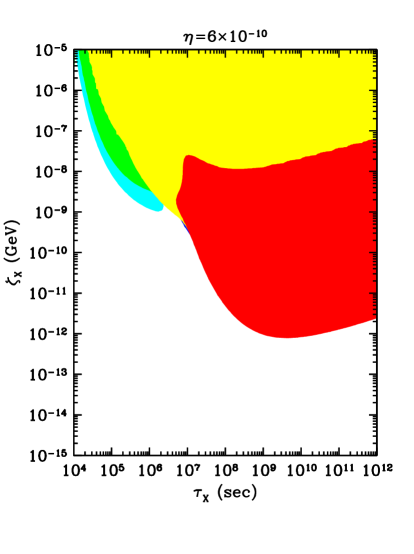
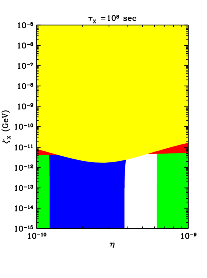
Figure 8: As in Figures 6 and 7 including the constraints from ⁶Li (dark red).

As already noted, if the observed light-element abundances retain their current central values, but the error budget shrinks, then the light-element data will be in discord with standard BBN. Decaying particles might provide one possible means of reconciling such light-element observations and theory. As an illustrative example, consider the case in which the CMB fixes $\eta_{10}=6$, and the observed light element abundances remain as above, but with the total error budget equal to that of the current statistical errors. Then ⁷Li and D would be in significant disagreement. One could, however, bring these nuclides and ⁴He into agreement by appealing to the decaying-particle scenario we have laid out here, the allowed region of parameter space still open being one in which a non-zero $\zeta_{X}$ is preferred. The new ⁷Li upper limit would eliminate low values of $\zeta_{X}$, allowing only a narrow band with $\zeta\approx 10^{-9}$. The observations would force us to live in the narrow channel where D production and destruction are nearly balanced, with a decaying particle lifetime $\tau_{X}\approx{3}\!\times\!10^{6}$ sec. In this regime, ⁴He is at its BBN value, because of its high photoerosion threshold, shown in Table 1. However, the more weakly bound ⁷Li is destroyed, at just the right level to bring the observations in accord with the D observations. This rather fine-tuned scenario is testable with ⁶Li observations. In this region of parameter space, we predict a ⁶Li abundance of ${\rm\mbox{${}^{6}${\rm Li}}/H}\approx 10^{-11}$ and $\mbox{${}^{6}${\rm Li}}/\mbox{${}^{7}${\rm Li}}\approx 0.03$. This ⁶Li abundance would appear as a pre-Galactic plateau in halo stars. Indeed, the ⁶Li level would be large enough to dominate the cosmic-ray component of ⁶Li over most of the Population II metallicity range.

6 Application to Cosmological Gravitinos

We now illustrate the impact of our calculations by discussing their implications for cosmological gravitinos. In conventional supergravity scenarios, the gravitino is expected to have a mass comparable to that of supersymmetric partners of standard Model particles, which should weigh less than about 1 TeV if they are to stabilize the gauge hierarchy [57]. Therefore, the gravitino is usually thought to weigh between about 100 GeV to 10 TeV, though both larger and smaller masses have sometimes been considered. The lightest supersymmetric particle (LSP) is generally thought to be the lightest neutralino $\chi$, a model-dependent mixture of the photino ${\tilde{\gamma}}$, the zino ${\tilde{Z}}$ and the neutral Higgsinos ${\tilde{H}}_{1,2}$ [58]. The LSP would be stable in models in which $R$ parity is conserved, as we assume here. On the other hand, the gravitino would be unstable, with a partial ${\tilde{G}}\to\chi+\gamma$ decay rate calculated to be

$$\Gamma(\tilde{G}\to\chi\gamma)\;=\;{1\over 4}\left({M_{\tilde{G}}^{3}\over M_{\rm P}^{2}}\right)O_{\chi\gamma}^{2},$$ (55)

where $O_{\chi\gamma}$ is the fraction of ${\tilde{\gamma}}$ in the wave function of the LSP $\chi$, and $M_{\rm P}$ is the Planck mass. In many models, the LSP is essentially a pure $U(1)$ gaugino (Bino) ${\tilde{B}}$, in which case $O_{\chi\gamma}=\cos^{2}\theta_{W}$ and the neutralino mixing does not suppress the gravitino decay rate (55). We assume for now that $\chi={\tilde{B}}$ and that no other gravitino decay modes are significant, in which case the gravitino lifetime is

$$\tau_{\tilde{G}}\;=\;2.9\times 10^{8}\left({100~{}{\rm GeV}\over M_{\tilde{G}}}\right)^{3}~{}{\rm s}.$$ (56)

We discuss later the modifications to our analysis needed if the LSP is essentially a pure Higgsino, another possibility sometimes considered, or if other decay modes are open to the gravitino.

The production of gravitinos in the early Universe has been the subject of heated discussion. An unavoidable contribution is thermal production [59, 8, 60, 61]. Here, we will apply our results in combination with the recent calculation in [61], which gives

$$Y_{\tilde{G}}\equiv{n_{\tilde{G}}\over n_{\gamma}}\;=\;1.2\times 10^{-11}\left(1+{m_{\widetilde{g}}^{2}\over 12m_{\tilde{G}}^{2}}\right)\times\left({T_{R}\over 10^{10}~{}{\rm GeV}}\right)$$ (57)

where $T_{R}$ is the maximum temperature reached in the early Universe. In conventional inflationary cosmology, $T_{R}$ is the reheating temperature achieved at the end of the inflationary epoch. In some inflationary scenarios, there may be additional gravitino production, either during the inflationary epoch or later, before thermalization is achieved. Either of these effects would only accentuate the potential problem we discuss below, and we do not consider such possibilities here.

In (57), $m_{\widetilde{g}}$ is the low-energy gluino mass. In supersymmetric models with gaugino mass unification, there is a definite relation between the gluino mass and the bino mass, which, at the one-loop order sufficient for our purposes, is $m_{\widetilde{g}}/m_{\widetilde{B}}\simeq\alpha_{3}(m_{\widetilde{g}})/\alpha_{1}$. Typically, this ratio is between 5 and 6. If the bino is the LSP, as we are presently considering, then $m_{\tilde{G}}\geq m_{\widetilde{B}}$. The middle term in (57) is therefore never larger than 4, and tends to unity for large gravitino masses. Thus we estimate

$$Y_{\tilde{G}}\;\simeq\;(0.7-2.7)\times 10^{-11}\times\left({T_{R}\over 10^{10}~{}{\rm GeV}}\right)$$ (58)

in this case.

The upper limit (1) can be expressed as a limit on $Y_{\tilde{G}}$:

$$Y_{\tilde{G}}<5\times 10^{-14}\times\left({100~{}{\rm GeV}\over m_{\tilde{G}}}\right)$$ (59)

Comparing the calculated abundance (58) with the upper limit (59), we infer the following upper limit on the reheating temperature $T_{R}$, for $M_{\tilde{G}}\sim 100~{}{\rm GeV}$:

$$T_{R}\;<\;(1.9-7.5)\times 10^{7}~{}{\rm GeV}$$ (60)

This upper limit is far smaller than the reheating temperature $T_{R}\sim 10^{12}$ GeV expected in conventional inflationary scenarios. As noted in the introduction, this bound places important constraints on models of baryo/leptogenesis.

We recall that the upper limit (60) comes from a combination of data and calculations of different light-element abundances. It could not be obtained by considering the deuterium abundance alone, as this would allow a ‘tail’ of the parameter space extending to large gravitino abundances $Y_{\tilde{G}}$, as well as an isolated ‘channel’ at large $Y_{\tilde{G}}$. The ‘tail’ cannot be excluded just by considering also the abundance of ⁴He, though the ‘channel’ probably can. However, as discussed earlier, the ‘tail’ can be excluded by also considering the ⁶Li abundance. We have already discussed why we think that measurements of the relevant photoreaction cross sections and the astrophysical data are now sufficiently reliable for the ⁶Li data to be regarded as a serious constraint.

As we commented at the end of the previous Section, if the observed light-element abundances were to retain their current central values while the error budget shrank, the light-element data would become inconsistent with standard BBN, and decaying particles might be able to reconcile such light-element observations with theory. This scenario would predict a lifetime $\tau_{\tilde{G}}\approx{3}\!\times\!10^{6}$ sec and an abundance $\zeta_{\tilde{G}}\approx 10^{-9}$ GeV. These constraints would place the gravitino mass at $M_{\tilde{G}}\approx 460$ GeV, with a relic abundance of $Y_{\tilde{G}}\approx{2}\!\times\!10^{-12}$, corresponding in turn to a reheating temperature $T_{R}\simeq{(0.8-3.1)}\!\times\!10^{9}$ GeV.

How might the potentially embarrassing conclusion (60) be avoided or evaded?

The first option one might consider is diluting the density of gravitinos by several orders of magnitude some time between their production at a temperature close to $T_{R}$ and the period when they decay. This large entropy release should certainly occur before BBN, i.e., when the age $t\mathrel{\hbox to0.0pt{\raise 2.15277pt\hbox{$<$}\hss}{\lower 2.15277pt\hbox{$\sim$}}}1$ s, in order to avoid destroying its predictions completely. Very likely, such a large entropy release would also have had to occur before baryogenesis, in order to avoid an unacceptable dilution of the primordially-generated baryon asymmetry. The latest epoch at which baryogenesis is seems likely to have occurred is the electroweak phase transition, which occurred when the age $t\sim 10^{-10}$ s. Afleck-Dine baryogenesis [40] offers one such possibility. In these models the Universe becomes dominated by the oscillation of a scalar field along a supersymmetric flat direction. In general, the net baryon asymmetry produced in these models can be quite large, actually necessitating late entropy production [62]. The dilution of the gravitino abundance would be an immediate consequence. The issue of gravitino production and dilution in connection with baryogenesis was recently considered [63] in the context of the pre-big bang scenario [64].

It is possible that the mass and decay modes of the gravitino are such that the bounds discussed here, which cover lifetimes from $10^{4}$ – $10^{12}$ s, become inapplicable. We see from (55) that the rate for ${\tilde{G}}\to\chi+\gamma$ decay would increase by three orders of magnitude if $M_{\tilde{G}}$ were one order of magnitude larger. In fact, a heavier gravitino might have additional decay modes open kinematically, possibly decreasing its lifetime by another two orders of magnitude if all the MSSM particle weighed less than $M_{\tilde{G}}$. If $\tau_{\tilde{G}}\sim 10^{4}$ s, as might occur if $M_{\tilde{G}}\sim 1$ TeV and it could decay into ${\tilde{X}_{EW}}+X_{EW}$ as well as $\chi+\gamma$, where $X_{EW}$ is any Standard Model particle with only electroweak interactions, our limits are significantly weakened. However, we remind the reader that outside the range $10^{4}$ – $10^{12}$ s other bounds come into play. At smaller lifetimes, hadronic decay products will upset the prediction of BBN [5, 6, 14]. From the recent results of [14], one finds that for lifetimes in the range 1 – $10^{4}$ s, the upper limit to $Y_{\tilde{G}}$ is of order $10^{-13}$, and this bound weakens at lower lifetimes. For $\tau<{\rm few}\times 10^{-2}$ s, the BBN limit disappears. Similarly, at longer lifetimes $>10^{12}$ s, there are non-negligible constraints from the observed gamma-ray background [65, 7, 66]. These are strongest for decay lifetimes of order the age of the Universe $\sim 10^{18}$ s, where the bound on $m_{\tilde{G}}Y_{\tilde{G}}$ is of order $10^{-16}$. At still longer lifetimes, the bound weaks quickly and becomes ineffective at lifetimes longer than about $10^{24}$ s.

Could the cosmological embarrassment be avoided if $M_{\tilde{G}}\ll 100$ GeV? In such a case, the gravitino would presumably be the LSP, and absolutely stable if $R$ parity is conserved, as we have been assuming. In fact, as argued in [61], a reheating temperature of order $10^{10}$ GeV would result in an acceptably large relic density of gravitinos. Converting the gravitino abundance in (58) to its contribution to closure density, one finds,

$$\Omega_{\tilde{G}}h^{2}=(0.026-0.1)\times\left({m_{\tilde{G}}\over 100{\rm\,Ge\kern-1.25ptV}}\right)\left({T_{R}\over 10^{10}{\rm\,Ge\kern-1.25ptV}}\right)$$ (61)

In this case, the lightest MSSM sparticle (presumably the lightest neutralino $\chi$) would be the next-to-lightest supersymmetric particle (NLSP), and would itself be unstable: the decay NLSP $\to\gamma+{\tilde{G}}$ would have a lifetime similar to (56), and the bound (57) could be applied to the NLSP abundance $Y_{NLSP}$, which in terms of $\Omega_{\chi}h^{2}$ is

$$\Omega_{\chi}h^{2}<2\times 10^{-4}.$$ (62)

However, suppressing $\Omega_{\chi}h^{2}$ to such a low value seems very difficult. Characteristic values of $\Omega_{\chi}h^{2}$ in the MSSM are ${\cal O}(0.01-10.0)$ [67], corresponding to $Y_{\chi}\sim 10^{-10}$, which is far above the bound (57). Indeed, in much of the phenomenologically allowed supersymmetric parameter space, the relic density is too large. Relic neutralino densities as low as (62) would require special parameter choices for which the neutralino is either primarily a massive Higgsino, in which case important coannihilation effects might suppress the abundance, or the neutralino mass happens to be very close to half the mass of the Heavy Higgs scalar and pseudo scalar, so that rapid $s$-channel annihilation reduces the neutralino density. In the former case, it is in fact unlikely that coannihilations are sufficiently strong to satisfy the bound (62), despite reducing the relic density to a level well below critical. In the latter case, however, very low relic densities are possible.

Could the cosmological embarrassment be avoided by altering the composition of the LSP into which the gravitino is supposed to decay? The gravitino decay amplitude could be suppressed, and the lifetime estimate (56) correspondingly increased, if the LSP did not have photino component, for example if it were essentially a pure Higgsino. However, in view of the discussion above, in realistic models it seems difficult to suppress the ${\tilde{G}}-\chi-\gamma$ coupling enough to increase the gravitino lifetime sufficiently to relax the bound (57) adequately, bearing in mind the bounds applicable for longer lifetimes.

Finally, we consider briefly the situation if $R$ parity is violated. First we consider $R$-violating decays of the lightest MSSM particle, assumed to be the lightest neutralino $\chi$. As discussed earlier, its abundance is likely to be $Y_{\chi}\mathrel{\hbox to0.0pt{\raise 2.15277pt\hbox{$>$}\hss}{\lower 2.15277pt\hbox{$\sim$}}}10^{-10}$, which conflicts with our bounds unless $\tau_{\chi}\mathrel{\hbox to0.0pt{\raise 2.15277pt\hbox{$<$}\hss}{\lower 2.15277pt\hbox{$\sim$}}}10^{4}$ s . Considering now the decays of the gravitino, assuming it to be heavier than $\chi$, there are two options to consider. The simplest possibility is that it decays in the same way as in the $R$-conserving case: ${\tilde{G}}\to\chi+\gamma$, etc., in which case the previous $R$-conserving gravitino analysis applies, and we again conclude that $\tau_{\tilde{G}}\mathrel{\hbox to0.0pt{\raise 2.15277pt\hbox{$<$}\hss}{\lower 2.15277pt\hbox{$\sim$}}}10^{4}$ s. Alternatively, the dominant ${\tilde{G}}$ decays might violate $R$ parity. In this case, the bound $\tau_{\chi}\mathrel{\hbox to0.0pt{\raise 2.15277pt\hbox{$<$}\hss}{\lower 2.15277pt\hbox{$\sim$}}}10^{4}$ s again applies, and, as discussed above, the same bound applies to the decays of the lightest MSSM sparticle.

7 Discussion and Conclusions

We have re-examined in this paper the upper limits on the possible abundance of any unstable massive relic particle that are provided by the success of Big-Bang Nucleosynthesis calculations. A new aspect of this work has been the use of cosmic microwave background data to constrain independently the baryon-to-photon ratio, which was not possible in previous studies of this problem. We have also incorporated in our analysis the an updated suite of photonuclear and nuclear cross sections, and calculated both analytically and numerically the network of reactions induced by electromagnetic showers that create and destroy the light elements deuterium, ³He, ⁴He, ⁶Li and ⁷Li.

It was pointed out in previous work that considerations of the deuterium abundance alone would allow certain exceptional regions of parameter space with relatively large abundances of unstable particles. However, as shown in this paper, considerations of the abundances of ⁴He and ⁶Li exclude these particular regions.

We have illustrated our results by applying them to massive gravitinos. If they weigh $\sim 100$ GeV, their primordial abundance $Y_{\tilde{G}}$ should have been $\mathrel{\hbox to0.0pt{\raise 2.15277pt\hbox{$<$}\hss}{\lower 2.15277pt\hbox{$\sim$}}}5\times 10^{-14}\times\left({100~{}{\rm GeV}/m_{\tilde{G}}}\right)$, corresponding to a reheating temperature $T_{R}\;<\;(1.9-7.5)\times 10^{7}$ GeV. This could present a potential difficulty for some models of inflation and leptogenesis. We have discussed various scenarios for evading this potential embarrassment, for example by varying the gravitino mass, or by postulating an alternative scenario for baryogenesis, such as non-thermal leptogenesis or the Affleck-Dine mechanism.

This example of the gravitino illustrates the power and importance of the cosmological upper limits on the abundances of unstable massive particles. Extensions of this analysis are clearly desirable. For example, it would be valuable to combine our analysis of electromagnetic decay cascades with a similar analysis of hadronic showers, a topic that lies beyond the scope of this paper.

Acknowledgments

We would like to thank Wilfried Buchmüller for helpful communications. The work of K.A.O. was partially supported by DOE grant DE–FG02–94ER–40823 at the Universoty of Minnesota. This work of BDF and RHC was supported by NSF grant AST 00-92939 at the University of Illinois.

Appendix A Cross Sections

Kawasaki, Kohri and Moroi [13] have provided a useful table of reactions and references to nuclear data. We have supplemented the data by using tabulations made by the National Nuclear Data Center (NNDC) [68] and the NACRE collaboration [69]. The relevant cross sections are listed here for convenience, and we refer the interested reader to the NNDC and NACRE websites for further references on the data.

We have computed thresholds and $|Q|$ values using the mass data of Audi and Wapstra[70], available on the US Nuclear Data Program website [71]. Reverse reaction data were sometimes available, in which cases we used detailed balance to transform the data into forward data. The equations of detailed balance for the reactions $\gamma+T\rightarrow A+B$ and $P+T\rightarrow A+B$ are:

$$\sigma_{\gamma+T\rightarrow A+B} = \frac{g_{A}g_{B}}{(1+\delta_{AB})g_{T}}\left(\frac{\mu E_{cm}(A,B)}{E_{\gamma}^{2}}\right)\sigma_{A+B\rightarrow T+\gamma}$$ (63)

$$\sigma_{P+T\rightarrow A+B} = \frac{(1+\delta_{PT})g_{A}g_{B}m_{A}m_{B}E_{cm}(A,B)}{(1+\delta_{AB})g_{P}g_{T}m_{P}m_{T}E_{cm}(P,T)}\sigma_{A+B\rightarrow P+T},$$ (64)

where the $g_{i}$ are the statistical weights of each species, $\mu$ is the reduced mass of the system $A+B$, and $E_{cm}(x,y)$ is the center-of-mass energy of the system $x+y$. See Blatt and Weisskopf [72] and Fowler, Caughlan, and Zimmerman [73] for discussions on these relations.

In the numerical fits, all energies are in MeV. In a few cases, which we have noted, the fits are those previously published. Otherwise, we have adopted a specific empirical form for the nonresonant parts of the cross sections. This form is the product of a power law in photon energy $E_{\gamma}$, and a power law in photon energy above threshold, $E_{\gamma}-|Q|$. We have found that expressions of this type provide a simple but accurate representation of the data.

1. d($\gamma$,n)p      $E_{\gamma,th}=|Q|=2.224573$ MeV [74].

   $$\!\!\!\!\!\!\!\!\!\!\!\!\!\!\!\!\!\sigma(E_{\gamma})=18.75{\rm mb}\!\!\left[\left(\frac{\sqrt{|Q|(E_{\gamma}-|Q|)}}{E}\right)^{\!\!3}\!\!+0.007947\left(\frac{\sqrt{|Q|(E_{\gamma}-|Q|)}}{E}\right)^{\!\!2}\!\!\frac{\left(\sqrt{|Q|}-\sqrt{0.037}\right)^{2}}{E_{\gamma}-(|Q|-0.037)}\right]$$

2. t($\gamma$,n)d      $E_{\gamma,th}=|Q|=6.257248$ MeV [75, 76].

   $$\!\!\!\!\!\!\!\!\!\!\!\!\!\!\!\!\!\sigma(E_{\gamma})=9.8{\rm mb}\frac{|Q|^{1.95}(E_{\gamma}-|Q|)^{1.65}}{E_{\gamma}^{3.6}}$$

3. t($\gamma$,np)n      $E_{\gamma,th}=|Q|=8.481821$ MeV [76].

   $$\!\!\!\!\!\!\!\!\!\!\!\!\!\!\!\!\!\sigma(E_{\gamma})=26.0{\rm mb}\frac{|Q|^{2.6}(E_{\gamma}-|Q|)^{2.3}}{E_{\gamma}^{4.9}}$$

4. ³He($\gamma$,p)d      $E_{\gamma,th}=|Q|=5.493485$ MeV [77, 78]. We use reverse reaction data from NACRE [69, 79].

   $$\!\!\!\!\!\!\!\!\!\!\!\!\!\!\!\!\!\sigma(E_{\gamma})=8.88{\rm mb}\frac{|Q|^{1.75}(E_{\gamma}-|Q|)^{1.65}}{E_{\gamma}^{3.4}}$$

5. ³He($\gamma$,np)p      $E_{\gamma,th}=|Q|=7.718058$ MeV [78, 80].

   $$\!\!\!\!\!\!\!\!\!\!\!\!\!\!\!\!\!\sigma(E_{\gamma})=16.7{\rm mb}\frac{|Q|^{1.95}(E_{\gamma}-|Q|)^{2.3}}{E_{\gamma}^{4.25}}$$

6. ⁴He($\gamma$,p)t      $E_{\gamma,th}=|Q|=19.813852$ MeV [81, 82, 83].

   $$\!\!\!\!\!\!\!\!\!\!\!\!\!\!\!\!\!\sigma(E_{\gamma})=19.5{\rm mb}\frac{|Q|^{3.5}(E_{\gamma}-|Q|)^{1.0}}{E_{\gamma}^{4.5}}$$

7. ⁴He($\gamma$,n)³He      $E_{\gamma,th}=|Q|=20.577615$ MeV [82, 84, 85, 86, 87].

   $$\!\!\!\!\!\!\!\!\!\!\!\!\!\!\!\!\!\sigma(E_{\gamma})=17.1{\rm mb}\frac{|Q|^{3.5}(E_{\gamma}-|Q|)^{1.0}}{E_{\gamma}^{4.5}}$$

8. ⁴He($\gamma$,d)d      $E_{\gamma,th}=|Q|=23.846527$ MeV [88, 89]. We use reverse reaction data from NACRE [69, 90].

   $$\!\!\!\!\!\!\!\!\!\!\!\!\!\!\!\!\!\sigma(E_{\gamma})=10.7{\rm mb}\frac{|Q|^{10.2}(E_{\gamma}-|Q|)^{3.4}}{E_{\gamma}^{13.6}}$$

9. ⁴He($\gamma$,np)d      $E_{\gamma,th}=|Q|=26.0711$ MeV [84].

   $$\!\!\!\!\!\!\!\!\!\!\!\!\!\!\!\!\!\sigma(E_{\gamma})=21.7{\rm mb}\frac{|Q|^{4.0}(E_{\gamma}-|Q|)^{3.0}}{E_{\gamma}^{7.0}}$$

10. ⁶Li($\gamma$,np)⁴He      $E_{\gamma,th}=|Q|=3.698892$ MeV [91, 92].

    $$\!\!\!\!\!\!\!\!\!\!\!\!\!\!\!\!\!\sigma(E_{\gamma})=104.{\rm mb}\frac{|Q|^{2.3}(E_{\gamma}-|Q|)^{4.7}}{E_{\gamma}^{7.0}}$$

11. ⁶Li($\gamma$,X)³A      $E_{\gamma,th}=|Q|=15.794685$ MeV [93].

    $$\!\!\!\!\!\!\!\!\!\!\!\!\!\!\!\!\!\sigma(E_{\gamma})=38.1{\rm mb}\frac{|Q|^{3.0}(E_{\gamma}-|Q|)^{2.0}}{E_{\gamma}^{5.0}}\times$$

    $$\!\!\!\!\!\!\!\!\!\!\!\!\!\!\!\!\!\left(3.7\exp{\left[-\frac{1}{2}\left(\frac{E_{\gamma}-19.0}{3.5}\right)^{2}\right]}+2.75\exp{\left[-\frac{1}{2}\left(\frac{E_{\gamma}-30.0}{3.0}\right)^{2}\right]}+2.2\exp{\left[-\frac{1}{2}\left(\frac{E_{\gamma}-43.0}{5.0}\right)^{2}\right]}\right)$$

12. ⁷Li($\gamma$,t)⁴He      $E_{\gamma,th}=|Q|=2.467032$ MeV      $E_{cm}=E_{\gamma}-|Q|$ [92]. We use reverse reaction data from NACRE [69], with modifications from Cyburt, Fields, and Olive [16, 94].

    $$\!\!\!\!\!\!\!\!\!\!\!\!\!\!\!\!\!\sigma(E_{\gamma})=0.105{\rm mb}\left(\frac{2371{\rm MeV^{2}}}{E_{\gamma}^{2}}\right)\exp{\left(\frac{-2.5954}{\sqrt{E_{cm}}}\right)}\times$$

    $$\!\!\!\!\!\!\!\!\!\!\!\exp{(-2.056E_{cm})}\left(1.+2.2875E_{cm}^{2}-1.1798E_{cm}^{3}+2.5279E_{cm}^{4}\right)$$

13. ⁷Li($\gamma$,n)⁶Li      $E_{\gamma,th}=|Q|=7.249962$ MeV [95, 96, 97].

    $$\!\!\!\!\!\!\!\!\!\!\!\!\!\!\!\!\!\sigma(E_{\gamma})=0.176{\rm mb}\frac{|Q|^{1.51}(E_{\gamma}-|Q|)^{0.49}}{E_{\gamma}^{2.0}}+1205{\rm mb}\frac{|Q|^{5.5}(E_{\gamma}-|Q|)^{5.0}}{E_{\gamma}^{10.5}}+\frac{0.06{\rm mb}}{1+\left(\frac{E_{cm}-7.46}{0.188}\right)^{2}}$$

14. ⁷Li($\gamma$,2np)⁴He      $E_{\gamma,th}=|Q|=10.948850$ MeV [92].

    $$\!\!\!\!\!\!\!\!\!\!\!\!\!\!\!\!\!\sigma(E_{\gamma})=122.{\rm mb}\frac{|Q|^{4.0}(E_{\gamma}-|Q|)^{3.0}}{E_{\gamma}^{7.0}}$$

15. ⁷Be($\gamma$,³He)⁴He      $E_{\gamma,th}=|Q|=1.586627$ MeV      $E_{cm}=E_{\gamma}-|Q|$. We use reverse reaction data from NACRE [69], with modifications from Cyburt, Fields, and Olive [16, 98].

    $$\!\!\!\!\!\!\!\!\!\!\!\!\!\!\!\!\!\sigma(E_{\gamma})=0.504{\rm mb}\left(\frac{2371{\rm MeV^{2}}}{E_{\gamma}^{2}}\right)\exp{\left(\frac{-5.1909}{\sqrt{E_{cm}}}\right)}\times$$

    $$\!\!\!\!\!\!\!\!\!\!\!\exp{(-0.548E_{cm})}\left(1.-0.428E_{cm}^{2}+0.534E_{cm}^{3}-0.115E_{cm}^{4}\right)$$

16. ⁷Be($\gamma$,p)⁶Li      $E_{\gamma,th}=|Q|=5.605794$ MeV. We use reverse reaction data from NACRE [69, 99].

    $$\!\!\!\!\!\!\!\!\!\!\!\!\!\!\!\!\!\sigma(E_{\gamma})=32.6{\rm mb}\frac{|Q|^{10.0}(E_{\gamma}-|Q|)^{2.0}}{E_{\gamma}^{12.0}}+{2.27}\!\times\!10^{6}{\rm mb}\frac{|Q|^{8.8335}(E_{\gamma}-|Q|)^{13.0}}{E_{\gamma}^{21.8335}}$$

17. ⁷Be($\gamma$,2pn)⁴He      $E_{\gamma,th}=|Q|=9.30468$ MeV. No data exist. We assume isospin symmetry and use the data for the reaction $\mbox{${}^{7}${\rm Li}}(\gamma,2np)\mbox{${}^{4}${\rm He}}$ [92].

    $$\!\!\!\!\!\!\!\!\!\!\!\!\!\!\!\!\!\sigma(E_{\gamma})=133.{\rm mb}\frac{|Q|^{4.0}(E_{\gamma}-|Q|)^{3.0}}{E_{\gamma}^{7.0}}$$

18. ⁴He(t,n)⁶Li      $E_{p,th}=8.386972$ MeV   $|Q|=4.78293$ MeV   $E_{cm}=\frac{m_{4}}{m_{4}+m_{t}}E_{p}$. We use reverse reaction data [100].

    $$\!\!\!\!\!\!\!\!\!\!\!\!\!\!\!\!\!\sigma(E_{\gamma})=1940.{\rm mb}\frac{[(E_{cm}-|Q|)/|Q|]^{.75}}{1+\left(\frac{E_{cm}-5.03043}{.09}\right)^{2}}+46.2{\rm mb}\frac{[(E_{cm}-|Q|)/|Q|]^{.25}}{1+\left(\frac{E_{cm}-7.1329}{3.0}\right)^{2}}\\ +32.8{\rm mb}\frac{[(E_{cm}-|Q|)/|Q|]^{.5}}{1+\left(\frac{E_{cm}-7.5239}{25.0}\right)^{2}}$$

    

    Figure 9: Cross-section data for the reaction ⁴He(t,n)⁶Li are plotted versus the center-of-mass energy. The solid curve is the parameterization we use, whilst the dashed curve is that adopted in previous studies [12, 13].

19. ⁴He(³He,p)⁶Li      $E_{p,th}=7.047667$ MeV   $|Q|=4.019167$ MeV   $E_{cm}=\frac{m_{4}}{m_{4}+m_{3}}E_{p}$. We use reverse reaction data [101].

    $$\!\!\!\!\!\!\!\!\!\!\!\!\!\!\!\!\!\sigma(E_{\gamma})=170.{\rm mb}\frac{[(E_{cm}-|Q|)/|Q|]^{.75}}{1+\left(\frac{E_{cm}-5.8192}{.6}\right)^{2}}+75.0{\rm mb}\frac{[(E_{cm}-|Q|)/|Q|]^{.25}}{1+\left(\frac{E_{cm}-7.5192}{3.0}\right)^{2}}\\ +32.1{\rm mb}\frac{[(E_{cm}-|Q|)/|Q|]^{.5}}{1+\left(\frac{E_{cm}-12.019}{11.5}\right)^{2}}$$

    

    Figure 10: Cross-section data for the reaction ⁴He(³He,p)⁶Li are plotted versus the center-of-mass energy. The solid curve is the parametrization we use, whilst the dashed curve is that adopted in previous studies [12, 13].

References

- [1] D. Lindley, Astrophys. J. 294 (1985) 1.
- [2] J. R. Ellis, D. V. Nanopoulos and S. Sarkar, Nucl. Phys. B 259 (1985) 175.
- [3] D. Lindley, Phys. Lett. B 171 (1986) 235.
- [4] R. J. Scherrer and M. S. Turner, Astrophys. J. 331 (1988) 19.
- [5] M. H. Reno and D. Seckel, Phys. Rev. D 37 (1988) 3441.
- [6] S. Dimopoulos, R. Esmailzadeh, L. J. Hall and G. D. Starkman, Nucl. Phys. B 311 (1989) 699.
- [7] J. Ellis et al., Nucl. Phys. B 337, 399 (1992).
- [8] M. Kawasaki and T. Moroi, Prog. Theor. Phys. 93 (1995) 879 [arXiv:hep-ph/9403364].
- [9] M. Kawasaki and T. Moroi, Astrophys. J. 452, 506 (1995) [arXiv:astro-ph/9412055].
- [10] R. J. Protheroe, T. Stanev and V. S. Berezinsky, Phys. Rev. D 51, 4134 (1995) [arXiv:astro-ph/9409004].
- [11] E. Holtmann, M. Kawasaki, K. Kohri and T. Moroi, Phys. Rev. D 60, 023506 (1999) [arXiv:hep-ph/9805405].
- [12] K. Jedamzik, Phys. Rev. Lett. 84, 3248 (2000).
- [13] M. Kawasaki, K. Kohri and T. Moroi, Phys. Rev. D 63 (2001) 103502 [arXiv:hep-ph/0012279].
- [14] K. Kohri, Phys. Rev. D 64 (2001) 043515 [arXiv:astro-ph/0103411].
- [15] T. P. Walker, G. Steigman, D. N. Schramm, K. A. Olive and H. S. Kang, Astrophys. J. 376 (1991) 51; D. N. Schramm and M. S. Turner, Rev. Mod. Phys. 70 (1998) 303 [arXiv:astro-ph/9706069]; K. A. Olive, G. Steigman and T. P. Walker, Phys. Rept. 333, 389 (2000) [arXiv:astro-ph/9905320]; K. M. Nollett and S. Burles, Phys. Rev. D 61 (2000) 123505 [arXiv:astro-ph/0001440]; A. Coc, E. Vangioni-Flam, M. Casse and M. Rabiet, Phys. Rev. D 65, 043510 (2002); B.D. Fields and S. Sarkar in: K. Hagiwara et al. [Particle Data Group Collaboration], Phys. Rev. D 66 (2002) 010001.
- [16] R. H. Cyburt, B. D. Fields and K. A. Olive, New Astron. 6 (1996) 215 [arXiv:astro-ph/0102179].
- [17] R. H. Cyburt, B. D. Fields and K. A. Olive, Astropart. Phys. 17 (2002) 87 [arXiv:astro-ph/0105397].
- [18] C. Pryke, N. W. Halverson, E. M. Leitch, J. Kovac, J. E. Carlstrom, W. L. Holzapfel and M. Dragovan, Astrophys. J. 568 (2002) 46 [arXiv:astro-ph/0104490].
- [19] J. L. Sievers et al., arXiv:astro-ph/0205387.
- [20] C. B. Netterfield et al. [Boomerang Collaboration], Astrophys. J. 571 (2002) 604 [arXiv:astro-ph/0104460].
- [21] M. E. Abroe et al., Mon. Not. Roy. Astron. Soc. 334 (2002) 11 [arXiv:astro-ph/0111010].
- [22] J. A. Rubino-Martin et al., arXiv:astro-ph/0205367.
- [23] E. Vangioni-Flam, K. A. Olive, B. D. Fields and M. Casse, arXiv:astro-ph/0207583.
- [24] D. V. Nanopoulos, K. A. Olive and M. Srednicki, Phys. Lett. B 127 (1983) 30.
- [25] J. R. Ellis, J. S. Hagelin, D. V. Nanopoulos, K. A. Olive and M. Srednicki, Nucl. Phys. B 238 (1984) 453.
- [26] J. R. Ellis, J. E. Kim and D. V. Nanopoulos, Phys. Lett. B 145 (1984) 181.
- [27] R. Juszkiewicz, J. Silk and A. Stebbins, Phys. Lett. B 158 (1985) 463.
- [28] M. Kawasaki and K. Sato, Phys. Lett. B 189 (1987) 23.
- [29] T. Moroi, H. Murayama and M. Yamaguchi, Phys. Lett. B 303 (1993) 289.
- [30] T. Moroi, arXiv:hep-ph/9503210.
- [31] J. R. Ellis, D. V. Nanopoulos, K. A. Olive and S. J. Rey, Astropart. Phys. 4 (1996) 371 [arXiv:hep-ph/9505438].
- [32] M. Bolz, A. Brandenburg and W. Buchmuller, Nucl. Phys. B 606 (2001) 518 [arXiv:hep-ph/0012052].
- [33] A.D. Linde, Particle Physics And Inflationary Cosmology, Harwood (1990); K. A. Olive, Phys. Rept. 190 (1990) 307; D. H. Lyth and A. Riotto, Phys. Rept. 314 (1999) 1 [arXiv:hep-ph/9807278].
- [34] M. Fukugita and T. Yanagida, Phys. Lett. B 174, 45 (1986).
- [35] M. A. Luty, Phys. Rev. D 45, 455 (1992).
- [36] B. A. Campbell, S. Davidson and K. A. Olive, Nucl. Phys. B 399, 111 (1993) [arXiv:hep-ph/9302223].
- [37] A. D. Dolgov and A. D. Linde, Phys. Lett. B 116 (1982) 329; D. V. Nanopoulos, K. A. Olive and M. Srednicki, Phys. Lett. B 127 (1983) 30; S. Dodelson, Phys. Rev. D 37 (1988) 2059; J. Yokoyama, H. Kodama, K. Sato and N. Sato, Int. J. Mod. Phys. A 2 (1987) 1809.
- [38] T. Asaka, K. Hamaguchi, M. Kawasaki and T. Yanagida, Phys. Lett. B 464 (1999) 12 [arXiv:hep-ph/9906366]; Phys. Rev. D 61 (2000) 083512 [arXiv:hep-ph/9907559].
- [39] G. F. Giudice, M. Peloso, A. Riotto and I. Tkachev, JHEP 9908 (1999) 014 [arXiv:hep-ph/9905242].
- [40] I. Affleck and M. Dine, Nucl. Phys. B 249 (1985) 361.
- [41] H. Murayama and T. Yanagida, Phys. Lett. B 322 (1994) 349 [arXiv:hep-ph/9310297]; M. Fujii, K. Hamaguchi and T. Yanagida, Phys. Rev. D 63 (2001) 123513 [arXiv:hep-ph/0102187].
- [42] J. M. O’Meara, D. Tytler, D. Kirkman, N. Suzuki, J. X. Prochaska, D. Lubin and A. M. Wolfe, Astrophys. J. 552, 718 (2001) [arXiv:astro-ph/0011179].
- [43] D. Tytler, J. M. O’Meara, N. Suzuki, and D. Lubin, Phys. Rept., 333, 409 (2000)
- [44] M. Pettini and D. V. Bowen, Astrophys. J. 560, 41 (2001) [arXiv:astro-ph/0104474]; S. D’Odorico, M. Dessauges-Zavadsky, and P. Molaro, A.A., 368, L21 (2001).
- [45] B. D. Fields, K. A. Olive, J. Silk, M. Cassé and E. Vangioni-Flam, Astrophys. J., 563, 653 (2001).
- [46] J. L. Linsky, Space Science Reviews, 84, 285 (1998).
- [47] B. D. Fields and K. A. Olive, Astrophys. J. 506, 177 (1998) [arXiv:astro-ph/9803297].
- [48] K.A. Olive, and E. Skillman, New Astronomy, 6, 119 (2001).
- [49] Y. I. Izotov and T. X. Thuan, Astrophys. J. 500, 188 (1998); Y. I. Izotov, T. X. Thuan, and V. A. Lipovetsky, Astrophys. J. 108, 1 (1997); Y. I. Izotov, T. X. Thuan, and V. A. Lipovetsky, Astrophys. J. 435, 647 (1994).
- [50] M. Peimbert, A. Peimbert and M.T. Ruiz, Astrophys. J. 541, 688 (2000); A. Peimbert, M. Peimbert and V. Luridiana, Astrophys. J. 565, 668 (2002).
- [51] T. M. Bania, R. T. Rood and D. S. Balser, Nature, 415, 54 (2002).
- [52] S.G. Ryan et al., Astrophys. J., 523, L57 (2000).
- [53] P. Bonifacio, et al., Astron. Astrophys., 390, 91 (2002).
- [54] V.V. Smith, D.L. Lambert, and P.E. Nissen, Astrophys. J. 408, 262 (1993); Astrophys. J. 506, 405 (1998); L.M. Hobbs and J.A. Thorburn, Astrophys. J. Lett., 428, L25 (1994); Astrophys. J. 491, 772 (1997); R. Cayrel, M. Spite, F. Spite, E. Vangioni-Flam, M. Cassé, and J. Audouze, Astron. Astrophys. 343, 923 (1999).
- [55] B. D. Fields and K. A. Olive, New Astronomy, 4, 255 (1999); E. Vangioni-Flam, M. Casse, R. Cayrel, J. Audouze, M. Spite, F. Spite, New Astronomy, 4, 245 (1999).
- [56] L. Brown and D.N. Schramm, Astrophys. J. 329, L103 (1988).
- [57] L. Maiani, Proceedings of the 1979 Gif-sur-Yvette Summer School On Particle Physics, 1; G. ’t Hooft, in Recent Developments in Gauge Theories, Proceedings of the Nato Advanced Study Institute, Cargese, 1979, eds. G. ’t Hooft et al., (Plenum Press, NY, 1980); E. Witten, Phys. Lett. B105, 267 (1981).
- [58] J. Ellis, J.S. Hagelin, D.V. Nanopoulos, K.A. Olive and M. Srednicki, Nucl. Phys. B238, 453 (1984).
- [59] J. R. Ellis, J. E. Kim and D. V. Nanopoulos, Phys. Lett. B 145 (1984) 181.
- [60] J. R. Ellis, D. V. Nanopoulos, K. A. Olive and S. J. Rey, Astropart. Phys. 4 (1996) 371 [arXiv:hep-ph/9505438].
- [61] M. Bolz, A. Brandenburg and W. Buchmuller, Nucl. Phys. B 606 (2001) 518 [arXiv:hep-ph/0012052].
- [62] J. R. Ellis, D. V. Nanopoulos and K. A. Olive, Phys. Lett. B 184 (1987) 37; J. R. Ellis, K. Enqvist, D. V. Nanopoulos and K. A. Olive, Phys. Lett. B 191 (1987) 343; B. A. Campbell, M. K. Gaillard, H. Murayama and K. A. Olive, Nucl. Phys. B 538 (1999) 351 [arXiv:hep-ph/9805300].
- [63] A. Buonanno, M. Lemoine and K. A. Olive, Phys. Rev. D 62 (2000) 083513 [arXiv:hep-th/0006054].
- [64] G. Veneziano, Phys. Lett. B 265 (1991) 287; M. Gasperini and G. Veneziano, Astropart. Phys. 1 (1993) 317 [arXiv:hep-th/9211021].
- [65] J. E. Gunn, B. W. Lee, I. Lerche, D. N. Schramm and G. Steigman, Astrophys. J. 223 (1978) 1015.
- [66] G. D. Kribs and I. Z. Rothstein, Phys. Rev. D 55 (1997) 4435 [Erratum-ibid. D 56 (1997) 1822] [arXiv:hep-ph/9610468].
- [67] J. R. Ellis, K. A. Olive and Y. Santoso, New J. Phys. 4 (2002) 32 [arXiv:hep-ph/0202110]; Phys. Lett. B 539 (2002) 107 [arXiv:hep-ph/0204192]; J. Ellis, T. Falk, K. A. Olive and Y. Santoso, arXiv:hep-ph/0210205.
- [68] Nuclear Data Centers Network, EXFOR Systems Manual: Nuclear Reaction Data Exchange Format, Report BNL-NCS-63330 (1996), compiled and edited by V. McLane, National Nuclear Data Center, Brookhaven National Laboratory, USA; see also the website: http://www.nndc.bnl.gov/nndc/exfor/.
- [69] C. Angulo et al., Nucl. Phys. A 656, 3 (1999); see also the website http://pntpm.ulb.ac.be/nacre.htm.
- [70] G. Audi and A.H. Wapstra, Nucl. Phys A 595, 409 (1995).
- [71] US Nuclear Data Program, http://www.nndc.bnl.gov/usndp/.
- [72] J.M. Blatt and V.F. Weisskopf, Theoretical Nuclear Physics, Springer-Verlag, New York (1979).
- [73] W.A. Fowler, G.R. Caughlan and B.A. Zimmerman, Annual Rev. of Astron. and Astrophys. 5, 525 (1967).
- [74] R.D. Evans, The Atomic Nucleus, McGraw-Hill, New York (1955).
- [75] R. Pfeiffer, Z. Phys. 208, 129 (1968).
- [76] D.D. Faul et al., Phys. Rev. Lett. 44, 129 (1980).
- [77] N.M. O’Fallon, L.J. Koester and J.H. Smith, Phys. Rev. C 5, 1926 (1972).
- [78] A.N. Gorbunov and A.T. Varfolomeev, Phys. Lett. 11, 137 (1964).
- [79] G.M. Griffiths, E.A. Larson and L.P. Robertson, Can. J. Phys. 40, 402 (1962); G.M. Griffiths, M. Lal and C.D. Scarfe, Can. J. Phys. 41, 724 (1963); J.B. Warren et al., Phys. Rev. 132, 1691 (1963); B.L. Berman, L.J. Koester Jr. and J.H. Smith, Phys. Rev.133, B117 (1964); V.N. Fetisov, A.N. Gorbunov and A.T. Varflomeev, Nucl. Phys. 71, 305 (1965); J.R. Stewart, R.C. Morrison and J.S. O’Connell, Phys. Rev.138, B372 (1965); W. Wolfli et al., Helv. Phys. Acta 40, 946 (1967); K.N. Geller, E.G. Muirhead and L.D. Cohen, Nucl. Phys. A 96, 397 (1967); G.J. Schmid et al., Phys. Rev. C 52, R1732 (1995).
- [80] H.M. Gertenberg and J.S. O’Connell, Phys. Rev. 144, 834 (1966).
- [81] Y.M. Arkatov et al., Ukrainskii Fizichnii Zhurnal 23, 1818 (1978).
- [82] A.N. Gorbunov, Phys. Lett. B 27, 436 (1968).
- [83] R. Bernabei et al., Phys. Rev. C 38, 1990 (1988).
- [84] B.L. Berman et al., Phys. Rev. C 22, 2273 (1980).
- [85] Y.M. Arkatov et al., Zhurnal Eksper. i Teoret. Fiz., Pisma v Redakt. 28, 710 (1978).
- [86] J.D. Irish et al., Can. Jour. Phys. 53, 802 (1975).
- [87] C.K. Malcom et al., Phys. Lett. B 322, 47 (1973).
- [88] Y.M. Arkatov et al., UFZ 23, 919 (1978).
- [89] Y.M. Arkatov et al., Sov. Jour. Nucl. Phys. 31, 157 (1980).
- [90] R.W. Zurmuhle, W.E. Stephens, and H.H. Staub, Phys. Rev. 132, 751 (1963); W.E. Meyerhof et al., Nucl. Phys. A 131, 489 (1969); F.J. Wilkinson III and F.E. Cecil, Phys. Rev. C 31, 2036 (1985); H.R. Weller et al., Phys. Rev. C 34, 32 (1986); C.A. Barnes et al., Phys. Lett. B 197, 315 (1987).
- [91] B.L. Berman et al., Phys. Rev. Lett. 15, 727 (1965).
- [92] V.V. Varlamov et al., Fotojad. Dannye - Photodisintegration of Lithium, Suppl., Moscow (1986).
- [93] V.P. Denisov et al., Yadernaya Fizika 5, 498 (1967).
- [94] G. M. Griffiths et al., Can. J. Phys. 39, 1397 (1961); S. Burzynski et al., Nucl. Phys. A 473, 179 (1987); U. Schröder et al., Phys. Lett. B 192, 55 (1987); C. R. Brune, R. W. Kavanagh and C. Rolfs, Phys. Rev. C 50, 2205 (1994).
- [95] S. Karataglidis et al., Nucl. Phys. A 501, 108 (1989).
- [96] R.L. Bramblett et al., Int. Conf. on Photonuclear Reactions, Pacific Grove (1973).
- [97] L. Green and D.J. Donahue, Phys. Rev. 135, 701 (1964).
- [98] H. D. Holmgren and R. L. Johnston, Phys. Rev. 113 (1959) 2556; P.D. Parker and R.W. Kavanagh, Phys. Rev. 131 (1963) 2578; K. Nagatani, M.R. Dwarakanath and D. Ashery, Nucl. Phys. A 128 (1969) 325; H. Kraewinkel et al., Z. Phys. A 304 (1982) 307; J. L. Osborne et al., Phys. Rev. Lett. 48 (1982) 1664; R. G. H. Robertson et al., Phys. Rev. C 27 (1983) 11; T. K. Alexander et al., Nucl. Phys. A427 (1984) 526; M. Hilgemeier et al., Z. Phys. A 329 (1988) 243.
- [99] Z.E. Switkowski et al., Nucl. Phys. A 331, 50 (1979); F.C. Barker, Aust. J. Phys. 33, 159 (1980); F.E. Cecil et al., Nucl. Phys. A 539, 75 (1992).
- [100] W.P. Poenitz, Z. Phys. 268, 359 (1974); J.C. Overley, R.M. Sealock and D.H. Ehlers, Nucl. Phys. A 221, 573 (1974); C.M. Bartle, Nucl. Instr. Meth. 121, 119 (1974); G.P. Lamaze, Nuclear Science and Engineering 68, 183 (1978); C. Renner et al., Bulletin of the American Physical Society 23, 526 (1978); J.B. Weddell and J.H. Roberts, Phys. Rev. 95, 117 (1954); F.L. Ribe, Phys. Rev. 103, 741 (1956); F. Gabbard, R.H. Davis and T.W. Bonner, Phys. Rev. 114, 210 (1959); S.J. Bame and R.L. Cubitt, Phys. Rev 114, 1580 (1959); R.B. Murray and H.W. Schmidt, Phys. Rev. 115, 1707 (1959); B.D. Kern and W.E. Kreger, Phys. Rev. 112, 926 (1958); H. Conde, S. Schwarz and N. Starfelt, Arkiv foer Fysik 29, 45 (1965); S. Schwarz, L.G. Stroemberg and A. Bergstroem, Nucl. Phys. 63, 593 (1965).
- [101] S.N. Abramovich et al., YK 4, 17 (1984); W. Gemeinhardt, D. Kamke and C. Von Rhoneck, Z. Phys. 197, 58 (1966); J.M.F. Jeronymo, G.S. Mani and A. Sadeghi, Nucl. Phys. 43, 424 (1963); O. Fiedler and P. Kunze, Nucl. Phys. A 96, 513 (1967); U. Fasoli, D. Toniolo and G. Zago, Phys. Lett. 8, 127 (1964); J.B Marion, G. Weber and F.S. Mozer, Phys. Rev. 104, 1402 (1956); C.R. Gould et al., Nuclear Science and Engineering 55, 267 (1974); H. Spinka, T. Tombrello and H. Winkler, Nucl. Phys. A 164, 1 (1971); C.S. Lin et al., Nucl. Phys. A 275, 93 (1976); T. Shinozuka, Y. Tanaka and K. Sugiyama, Nucl. Phys. A 326, 47 (1979); G.M. Temmer, Nucl. Reaction Mechanisms Conf., Padua (1962); A.J. Elwyn et al., Phys. Rev. C 20, 1984 (1979); M. Varnagy et al., Nucl. Inst. Meth. 119, 451 (1974); J. Szabo et al., Conf. on Nucl.Data for Sci.and Technol.,Antwerp (1982); J.U. Kwon, J.C. Kim and B.N. Sung, Nucl. Phys. A 493, 112 (1989).