Stationary models of relativistic magnetohydrodynamic jets

Abstract

Highly relativistic jets are most probably driven by strong magnetic fields and are launched from the accretion disk surrounding a central black hole.

In this paper we review some of our recent results considering the two-dimensional magnetic field structure and the dynamics of collimating relativistic jets. Applying the stationarity assumption enables us to calculate global solutions of the relevant MHD equations. The structure of the jet magnetosphere follows from the so called Grad-Shafranov equation for the force-balance between axisymmetric magnetic surfaces. The plasma dynamics along the magnetic field lines is given by the solution of the MHD wind equation. In the force-free assumption, which is appropriate for relativistic jets, both equations de-couple.

We discuss solutions of the Grad-Shafranov equation obtained in a general relativistic context applying the 3+1 formalism for Kerr geometry. These solutions extend from the inner light surface around the Kerr black hole to the asymptotic regime of a cylindrically collimated jet with a finite radius.

In a further step, we include differential rotation of the foot points of the field lines. In this case, the shape of the light surface is not known a priori and must be calculated in an iterative way. The solutions show that differentially rotating jets are collimated to smaller radii compared to jets with rigid rotation.

Considering the general relativistic MHD wind equation, we investigate the dynamics of the collimating jet, in particular the effects of Kerr metric on the acceleration. Temperature and density follow a power law versus radius. The jet magnetic (velocity) field is dominated by the toroidal (poloidal) component.

Having at hand a relativistic MHD jet solution, we calculate the thermal optically thin X-ray spectrum for the innermost hot part of the jet. Doppler shift and boosting is taken into account. For microquasars we obtain a jet X-ray luminosity $\approx 10^{33}\,{\rm erg\,s}^{-1}$. Iron emission lines are clearly visible.

1 Relativistic astrophysical jets

Relativistic jets originating in the close environment of a rotating black hole are observationally indicated for two categories of sources concerning mass and energy output. In active galactic nuclei (AGN), the jets are launched in the magnetized environment around a rotating, super massive black hole (Blandford & Payne 1982, Sanders et al. 1989). The discovery of Galactic microquasars has proven superluminal motion on a much smaller energy scale (Mirabel & Rodriguez 1994), the central engine, however, is believed to work similarly to the AGN.

From the observations we know that astrophysical jets are collimated to almost cylindrical shape. Relativistic jets are generally detected in non-thermal radio emission, clearly indicating the magnetic character of jet formation – magnetic acceleration and collimation. There is clear evidence that jet formation is always connected to the existence of an accretion disk. As the central object in AGN and microquasars is a black hole, the surrounding accretion disk is the only possible location for a magnetic field field generation. Considering the before mentioned observational constraints, it is clear that a theoretical, quantitative analysis of the jet structure in these sources must take into account both magnetohydrodynamic (MHD) effects and (general) relativity. Relativistic MHD implies that electric fields, which are unimportant in Newtonian MHD, cannot be neglected.

Due to the complexity of the MHD equations, all stationary, relativistic models of magnetic jets so far, rely on simplifying assumptions such as self-similarity (Contopoulos 1994), some other prescription of the field structure (Li 1993, Beskin 1997) or the restriction to asymptotic regimes (e.g. Appl & Camenzind 1993; Nitta 1997; Beskin & Malyshkin 2000). As relativistic jets must be highly magnetized, the force-free limit of MHD may be applied. This allows for a truly two-dimensional (2D) calculation of the field structure (Camenzind 1987; Fendt et al. 1995; Fendt 1997; Fendt & Memola 2001), in contrast to the self-similar treatment.

The stationarity assumption itself is essential in order to obtain a global solution of the equations. Yet, time-dependent MHD simulations of relativistic jet formation are limited in spatial scale and to a short time evolution (Koide et al. 2000). On the other hand, we do not really know whether a stationary MHD solution obtained is actually stable.

2 Stationary relativistic MHD

The axisymmetric, stationary electromagnetic equations in the context of Kerr metric were first derived by Znajek (1977). The more comprehensible formalism of a “3+1 split” has been introduced by Thorne et al. (see Thorne et al. 1986). Camenzind (1986, 1987) formulated a fully relativistic stationary description of axisymmetric MHD flows presenting solutions of the Grad-Shafranov and the wind equation. An essential step to obtain the global magnetic field structure is to take into account properly the regularity condition along the light surface. This matching problem of relativistic magnetospheres has been solved by Fendt et al. (1995). The general relativistic version of the Grad-Shafranov equation including inertial terms and entropy has been presented by Beskin & Pariev (1993). Solutions of the wind equation in Kerr geometry considering the stationary plasma motion along the magnetic field were obtained by Takahashi et al. (1990), however, mainly discussing the accretion flow onto the black hole.

2.1 Space-time around rotating black holes

In the 3+1 split the space-time around rotating black holes (mass $M$, angular momentum per unit mass $a=J/Mc$) can be described using the Boyer-Lindquist line element

$$ds^{2}=\alpha^{2}c^{2}dt^{2}-\tilde{\omega}^{2}\,(d\phi-\omega dt)^{2}-(\rho^{2}/\Delta)\,dr^{2}-\rho^{2}\,d\theta^{2}\,.$$ (1)

$t$ denotes a global time in which the system is stationary, $\phi$ is the angle around the symmetry axis, and $r,\theta$ are similar to the flat space spherical coordinates. The electromagnetic field $\vec{B},\vec{E}$, the current density $\vec{j}$, and the electric charge density $\rho_{\rm c}$ are measured by the ZAMO according to the locally flat Minkowski space. These local experiments are put together by a global observer at a certain global time using the lapse and shift function to transform from local to global frames. In spite of this transformation, Maxwell’s equations in the 3+1 split look similar to those in Minkowski space.

2.2 The cross–field force–balance

The axisymmetric field structure follows from the force-balance across magnetic flux surfaces. The magnetic flux function $\Psi(r,\theta)=\frac{1}{2\pi}\int{\vec{B}}_{\rm P}\cdot d{\vec{A}}$ measures the magnetic flux through a loop of the Killing vector $\vec{m}=\tilde{\omega}^{2}\nabla\phi$. Similarly, the total poloidal current is defined by integrating the poloidal current density over the same loop $I=-\int\alpha{\vec{j}}_{\rm P}\cdot d{\vec{A}}=-\frac{c}{2}\alpha\tilde{\omega}B_{\rm T}\,.$ The indices P and T denote the poloidal and toroidal components of a vector. In the force-free limit, $\rho_{\rm c}\vec{E}+\frac{1}{c}\vec{j}\times\vec{B}=0\,,$ we have $\vec{j}_{\rm P}\parallel\vec{B}_{\rm P}$ and, thus, $I=I(\Psi)$. For a degenerated magnetosphere, $|B^{2}-E^{2}|>>|\vec{E}\cdot\vec{B}|\simeq 0$ another conserved quantity can be derived. The derivative of the time component of the vector potential defines the iso-rotation parameter $\Omega_{\rm F}=\Omega_{\rm F}(\Psi)=-c(dA_{0}/d\Psi),$ which is sometimes interpreted as angular velocity of the magnetic field lines.

The force-balance across the field can be derived from the toroidal component of the stationary Ampère’s law and is commonly known as Grad-Shafranov equation (GSE) for the flux function $\Psi(r,\theta)$,

$$\tilde{\omega}\nabla\cdot\left({\alpha\,\frac{D}{\tilde{\omega}^{2}}}\nabla\Psi\right)=\tilde{\omega}\,\frac{\omega-\Omega_{\rm F}(\Psi)}{\alpha c^{2}}\Omega_{\rm F}^{\prime}(\Psi)\,|\nabla\Psi|^{2}-\frac{1}{\alpha\tilde{\omega}}\frac{2}{c^{2}}\;I(\Psi)\,I^{\prime}(\Psi)$$ (2)

(see Okamoto 1992). Here, $D\equiv 1-\left({\tilde{\omega}}/{\tilde{\omega}_{\rm L}}\right)^{2}$ The ’ denotes derivatives $d/d\Psi$, and $\tilde{\omega}_{\rm L}(\Psi)$ the position of the two light surfaces , $\tilde{\omega}_{\rm L}^{2}=\left(\pm{\alpha\,c}/({\Omega_{\rm F}-\omega})\right)^{2}\,.$

2.3 Jet acceleration – the force–balance along the field

The stationary, polytropic, general relativistic MHD flow along axisymmetric flux surfaces $\Psi$ can be described by the wind equation

$$u_{\rm p}^{2}+1=\left(\frac{E}{\mu}\right)^{2}\frac{k_{0}k_{2}-2k_{2}M^{2}-k_{4}M^{4}}{(k_{0}-M^{2})^{2}}$$ (3)

for the poloidal velocity $u_{\rm p}\equiv\gamma v_{\rm p}/c$ (Camenzind 1986, Takahashi et al. 1990). The Alfvén Mach number $M$ is defined via $M^{2}=4\mu nu_{\rm p}^{2}/\tilde{B}_{\rm p}^{2}$, with the proper particle density $n$, the specific enthalpy $\mu$, and the poloidal magnetic field $\tilde{B}_{\rm p}=B_{\rm P}/(g_{00)}+g_{03}\Omega_{\rm F})$, rescaled for mathematical convenience. The specific total energy density $E(\Psi)$ and total angular momentum density $L(\Psi)$ are conserved along the flux surfaces. For a polytropic gas law ($\Gamma\equiv n/m$), the wind equation can be converted into a polynomial equation $\sum_{i=0}^{2n+2m}A_{i}\,u_{\rm P}^{i/m}=0$ (Camenzind 1986), where the coefficients $A_{i}$ depend on the radius along $\Psi$, the field strength and the parameters $\Omega_{\rm F},E,L,\sigma_{\star}$. The magnetization $\sigma_{\star}(\Psi)$ measures the Poynting flux in terms of mass flux.

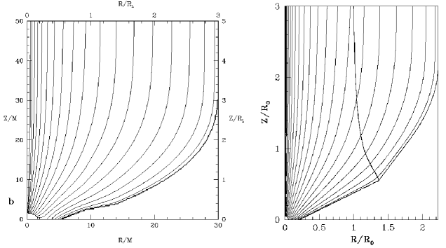
Figure 1: Axisymmetric magnetic field structure of relativistic jets $\Psi(R,Z)$. General relativistic jet magnetosphere around a rotating black hole with $a=0.8$, $\Omega_{\rm F}=$const. (left). Special relativistic magnetosphere with differential rotation $\Omega_{\rm F}(\Psi)$ (right).

3 The 2D structure of relativistic jet magnetospheres

We now discuss the GSE solution for a force-free, collimating jet in the general relativistic context (see Fendt 1997), assuming $\Omega_{F}(\Psi)=$const. As asymptotic boundary condition we apply the analytical, special relativistic 1D GSE solution of Appl & Camenzind (1993). Since $I=I(\Psi)$, this asymptotic solution provides the GSE source term also for the collimation region. The disk magnetic field distribution is parameterized as $\Psi\sim(x/b)^{m}/(1+(x/b)^{m})+\Psi_{H}$, Here, the magnetic flux anchored in the black hole is $\Psi_{H}=0.5$ with $m=3$ and a core radius $b$. The asymptotic jet radius can be parameterized in terms of the light cylinder radius $R_{L}$ or the gravitational radius $M$. For $a=0.8$, $(\Omega_{\rm F}/\Omega_{\rm H})=0.4$, the jet radius is $3\,R_{\rm L}$ corresponding to $30\,M$.

The main features of the calculated jet magnetosphere are the following (Fig. 1, left). The field lines originate near the inner light surface close to the rotating black hole and collimate to an asymptotic jet of finite radius of several (asymptotic) light cylinder radii. The solution is defined on a global scale, satisfying the regularity condition along the light surfaces. We find a rapid field collimation within $20\,M$ distance from the source. The near-disk solution has three different regimes. Here, the magnetic flux is either outgoing towards the asymptotic jet or in-going towards the black hole. But there exist also flux surfaces near the axis which not connected to the disk. Thus, if we imagine a mass flow associated with the field lines, we expect three different flow regimes – accretion, outflow, and a region empty of a plasma flow.

Extending our work on relativistic magnetospheres, we have investigated jets with non-constant $\Omega_{\rm F}(\Psi)$ (see Fendt & Memola 2001). Here, general relativity is not taken into account. Since astrophysical jets seem to be always connected to an accretion disk, differential rotation of the field lines should be a natural ingredient for any jet model. However, as a difficulty, then the position and shape of the light surface singularity is not known a priori, but have to be calculated iteratively with the field distribution. Similar to $I(\Psi)$, also the rotation law $\Omega_{\rm F}(\Psi)$ can be taken from the asymptotic GSE solution.

The calculated magnetic field structure is shown in Fig. 1 (right). The differentially rotating magnetosphere is collimated into a narrower jet. This, however, can be balanced by an increase of electric current. Comparison to high-resolution radio observations of the M87 jet (Junor et al. 1999) shows good agreement in the collimation distance. For M87 we derive a light cylinder (jet) radius of 50 (120) Schwarzschild radii.

The field structure is governed by $I(\Psi)$ and $\Omega_{\rm F}(\Psi)$. In combination with the disk magnetic flux distribution this allows to determine the magnetic angular momentum loss from the disk in the jet and the toroidal magnetic field along the disk. The angular momentum flux per unit time per unit radius is $d\dot{J}/dx=-xB_{\rm z}I(x)$ along the disk. In our solutions, most of the magnetic angular momentum is lost in the outer part of the disk (Fendt & Memola 2001).

3.1 The MHD wind solution in Kerr metric

Here, we discuss solutions of the stationary, general relativistic, MHD wind equation (3) along collimating magnetic flux surfaces. The solutions are calculated on a global scale up to several 1000 gravitational radii. Different magnetic field geometries were investigated, parameterized by the shape of the magnetic flux surface and the flux distribution (Fendt & Greiner 2001, FG01).

Figure 2: MHD wind solution in Kerr metric ($a=0.8$). Shown is the normalized poloidal velocity $u_{\rm p}$ in the global frame (left) and the density (thick line) and temperature versus radius $x=r/M$ (right). The intersections of the physical wind branch with the secondary solution indicate the magnetosonic points. Dynamical parameters are (see FG01): $\sigma_{\star}=980$, $\Omega_{\rm F}=0.035$, injection sound speed $c_{\rm s\star}=0.05$, Alfvén radius $x_{\rm A}=22.9$, asymptotic velocity $u_{{\rm p}\infty}=2.53$, total energy $E/m_{p}c^{2}=2.79$, field distribution $z\sim x^{6/5}$ and $\tilde{B}_{\rm p}\sim x^{-2}$.

Applying microquasar parameters, we obtain the following results (Fig. 2). The solution passes all three critical points (slow, Alfvén and fast magnetosonic point). Substantial acceleration is achieved also beyond the Alfvén point due to the magnetic nozzle effect (Camenzind 1986, Li 1993). The temperature in the inner jet is up to $10^{11}$K. The jet injection radius is at $8.3\,M$. Comparison to solutions with smaller injection radius ($3.3\,M$) allows to clarify the role of general relativity for the jet acceleration. In this case, the asymptotic velocity is much higher due to the faster rotation $\Omega_{\rm F}$ at smaller radii. With $\Omega_{\rm F}=0.14$ the asymptotic velocity increases to $u_{\rm p}=8.48$ (FG01).

In the limit of Minkowski metric the jet magnetization can be low, although the asymptotic speed is the same as for Schwarzschild metric (FG01). The jet flow is not affected by gravity and, thus, needs less magnetic energy to gain the same asymptotic speed by magnetic acceleration. Solutions for different Kerr parameter $a$ show that the jet is faster for smaller $a$ (see FG01). The reason for this seems to be the fact that the effective potential of a black hole weakens for increasing values of $a$.

These results might not be surprising as just demonstrating the fact of a magnetically driven jet. MHD theory tells us that magnetic acceleration takes place mainly around the Alfvén point. If that is far out, the influence of general relativity must be marginal.

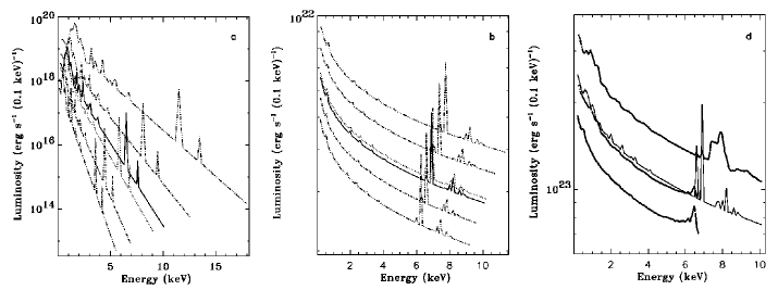
Figure 3: X-ray spectrum of a relativistic MHD wind solution for a microquasar. Shown is the luminosity of two volume elements along the jet with different temperature, $T=10^{7}$ K (left) and $T=10^{9}$ K (middle), and velocity for different inclination, $i=40^{o},20^{o},0^{o},-20^{o},-40^{o}$ (dashed curves from top to bottom), and in the rest-frame (thick curve). The right panel shows the overall spectrum of the red (blue) shifted side of the jet, $i=-20^{o}$ (top) and $i=-20^{o}$ (bottom), the combined spectrum (thick line middle) and the rest-frame spectrum (thin line middle).

3.2 X-rays as tracer for jet motion in microquasars?

The MHD wind solutions discussed above provide the flow dynamics along a prescribed poloidal magnetic field line with maximum temperatures up to $10^{11}$ K in the innermost part of the jet. Here, we calculate the thermal optically thin X-ray spectrum of such a jet. Prescribing the jet mass flow rate $\dot{M}_{\rm j}$ together with the shape of the field line, the wind solution gives a unique set of parameters of the flow. For each volume element of the expanding jet flow with decreasing temperature and density and increasing velocity we compute the continuum spectrum and the emission lines of an optically thin plasma (see Memola et al. 2002). The spectra of the single volumes are then put together to an overall spectrum taking into account the Doppler factor $D=(\gamma(1-\beta\cos\theta))^{-1},$ for shifting ($E_{o}=D\,E_{e}$) and boosting ($L_{o}(E_{o})=D^{3}\,L_{e}(E_{e})$) the emitted energy $E_{e}$ and luminosity $L_{e}$. These factors vary due to the different velocity $\beta$ of the matter in these volumes and the different inclination $\theta$ of the velocity vectors to the line of sight.

Figure 3 shows the spectra of two example volume elements of different temperature (and velocity) for different jet inclinations. The combined total spectrum of all volume elements within the collimating jet cone is shown in Fig. 3 (right). We find a X-ray luminosity $\sim 10^{33}$ ($\dot{M}_{\rm j}/10^{-8}\,{\rm M}_{\odot}{\rm yr}^{-1}){\rm erg\,s^{-1}}$ for a microquasar. The 6.6 and 6.9 keV emission lines can be identified as $K\alpha$ iron lines, while the one at 8.2 keV could be the $K\beta$. We emphasize that our approach is not a fit to certain observed spectra. In contrary, for the first time, for a jet flow with characteristics defined by the solution of the MHD wind equation, we derive its X-ray spectrum.

- [1] Appl, S., Camenzind, M., 1993, A&A, 274, 699
- [2] Beskin, V.S., Pariev, V.I., 1993, Physics Uspekhi, 36, 529
- [3] Beskin, V.S., 1997, Phys. Uspekhi, 40, 659
- [4] Beskin, V.S., Malyshkin, L. M., 2000, Astr. Lett., 26, 208
- [5] Blandford, R.D., Payne, D.G., 1982, MNRAS, 199, 883
- [6] Camenzind, M., 1986, A&A, 162, 32
- [7] Camenzind, M., 1987, A&A, 184, 341
- [8] Contopoulos, J., 1994, ApJ, 432, 508
- [9] Fendt, Ch., 1997, A&A, 319, 1025
- [10] Fendt, Ch., Camenzind, M., Appl, S., 1995, A&A, 300, 791
- [11] Fendt, Ch., Memola, E., 2001, A&A, 365, 631
- [12] Fendt, Ch., Greiner, J., 2001, A&A, 369, 308 (FG01)
- [13] Junor, W., Biretta J.A., Livio M., 1999, Nature, 401, 891
- [14] Koide, S., Meier D.L., Shibata K., Kudoh T., 2000, ApJ, 536, 668
- [15] Li, Z.-Y., 1993, ApJ, 415, 118
- [16] Memola, E., Fendt, Ch., Brinkmann, W., 2002, A&A, 385, 1089
- [17] Mirabel, I.F., Rodriguez, L.F., 1994, Nature, 371, L46
- [18] Nitta, S.-Y., 1997, MNRAS, 284, 899
- [19] Okamoto, I., 1992, MNRAS, 254, 192
- [20] Sanders, D.B., Phinney, E.S., Neugebauer, G., Soifer, B.T., Matthews, K., 1989, ApJ, 347, 29
- [21] Thorne, K.S., Price, R.H., Macdonald, D. (Eds), 1986, Black Holes: The membrane paradigm, Yale University Press, New Haven
- [22] Takahashi, M., Nitta, S., Tatematsu, Y., Tomimatsu, A., 1990, ApJ, 363, 206
- [23] Znajek, R.L., 1977, MNRAS, 179, 457