The Evolution of a Mass-Selected Sample of Early-Type Field Galaxies

Abstract

We investigate the evolution of mass-selected early-type field galaxies using a sample of 28 gravitational lenses spanning the redshift range $0\lesssim z\lesssim 1$. Based on the redshift-dependent intercept of the fundamental plane in the rest frame $B$ band, we measure an evolution rate of $d\log(M/L)_{B}/dz=-0.56\pm 0.04$ (all errors are $1\sigma$ unless noted) if we directly compare to the local intercept measured from the Coma cluster. Re-fitting the local intercept helps minimize potential systematic errors, and yields an evolution rate of $d\log(M/L)_{B}/dz=-0.54\pm 0.09$. An evolution analysis of properly-corrected aperture mass-to-light ratios (defined by the lensed image separations) is closely related to the Faber-Jackson relation. In rest frame $B$ band we find an evolution rate of $d\log(M/L)_{B}/dz=-0.41\pm 0.21$, a present-day characteristic magnitude of $M_{*0}=-19.70+5\log h\pm 0.29$ (assuming a characteristic velocity dispersion of $\sigma_{DM*}=225\,{\rm km\,s^{-1}}$), and a Faber-Jackson slope of $\gamma_{FJ}=3.29\pm 0.58$. The measured evolution rates favor old stellar populations (mean formation redshift $\langle z_{f}\rangle>1.8$ at $2\sigma$ confidence for a Salpeter initial mass function and a flat $\Omega_{m}=0.3$ cosmology) among early-type field galaxies, and argue against significant episodes of star formation at $z<1$.

1 Introduction

In recent years, enormous progress has been made in tracing the evolution of the formation rate of massive stars with cosmic epoch (e.g., Madau, Pozzetti & Dickinson 1998 and references therein). Although these massive stars initially dominate the luminosity of stellar systems, particularly the ionizing luminosity, they represent a negligible fraction of the overall stellar mass in galaxies. Tracing the formation history of the lower mass stars is more difficult, but it is necessary if we are to have a complete picture of the star-formation history of the universe. One means for tracing the formation history of these stars is to follow the evolution of the mass-to-light ratios of galaxies with redshift. Because studying evolution using mass-to-light ratios requires a determination of the galaxy mass or a surrogate for the mass, this approach has developed slowly due to the difficulty in measuring the rotation curves (e.g., Vogt et al. 1996; Ziegler et al. 2002) or velocity dispersions (e.g., van Dokkum & Franx 1996) of galaxies at intermediate redshift.

Most of the progress has been made in studies of early-type galaxies. It has long been known that the remarkable homogeneity of these galaxies is a powerful constraint on formation models. First, the population exhibits very uniform colors both locally (e.g., Bower, Lucey & Ellis 1992) and at $z\sim 1$ (e.g., Ellis et al. 1997; Stanford, Eisenhardt & Dickinson 1998). Second, the early-type galaxies follow a tight correlation among central velocity dispersion, effective (half-light) radius, and surface brightness known as the fundamental plane (FP; Djorgovski & Davis 1987; Dressler et al. 1987). The scatter in the FP, which is closely related to the scatter in mass-to-light ratio, is locally small (e.g., Jorgensen, Franx & Kjaergaard 1996; Pahre, Djorgovski & de Carvalho 1998a; Bernardi et al. 2001), does not evolve significantly with redshift (e.g., van Dokkum & Franx 1996; Kelson et al. 1997; Pahre, Djorgovski & de Carvalho 2001), and shows little dependence on the environment (e.g., van Dokkum et al. 1998, 2001; Kochanek et al. 2000; Treu et al. 2001).

In modern theoretical models of galaxy formation, (e.g., White & Rees 1978; Davis et al. 1985; Kauffmann, White & Guiderdoni 1993; Cole et al. 1994; Kauffmann 1996), early-type galaxies are assembled via the mergers of late-type galaxies. Support for the hierarchical clustering model is provided by the observation that high-redshift clusters exhibit both increased merger rates (e.g., Lavery & Henry 1988; Dressler et al. 1994; Couch et al. 1998; van Dokkum et al. 1999, 2000) and decreased fractions of elliptical galaxies (e.g., Dressler et al. 1997; Couch et al. 1998; van Dokkum et al. 2000; see Fabricant, Franx & van Dokkum 2000 for insightful criticism) compared to their present-day counterparts. Semi-analytic CDM models (Baugh, Cole & Frenk 1996; Kauffmann 1996; Kauffman & Charlot 1998) further predict that early-type galaxies in the field should contain recently-formed ($z_{f}<1$) stellar populations, while those in clusters should have significantly older stellar populations. Local observational studies have difficulty separating the effects of age and metallicity (e.g., Faber 1973; Worthey 1994; Trager et al. 2000), but such degeneracies can be broken by measuring the evolution of mass-to-light ratios with redshift.

Morphological evolution can complicate attempts to study the stellar evolution if the number density of massive early-type galaxies evolves rapidly to redshift unity (e.g., Kauffmann 1996; van Dokkum & Franx 2001). For example, a paucity of E/S0 galaxies with young blue stars out to $z\sim 1$ may be produced by several different star-formation and merger histories. First, all early-type galaxies could have been assembled at very high redshift (e.g., $z\sim 3$). Here the stars of $z<1$ E/S0 galaxies look old because the galaxies themselves are old. Second, some early-type galaxies could have been assembled more recently (e.g., $z<1$) from galaxies that had old stars and no ongoing star-formation prior to the merger (e.g., van Dokkum et al. 1999, 2000). The assembly age of the E/S0 galaxies would be much lower than the stellar age in this scenario, but the stellar age derived from early-types out to $z\sim 1$ would accurately represent the stellar age among all progenitors of present-day early-type galaxies. Finally, some E/S0s could be assembled at $z<1$ through the mergers of star-forming late-type galaxies. In this case, a range of assembly times leads to an evolving distribution of stellar formation times for the early-type population. As one moves to higher redshifts, the younger present-day early-type galaxies have yet to be assembled from their smaller, star-forming progenitor galaxies and do not appear in the higher redshift E/S0 samples. Consequently, by considering only early-type galaxies out to $z\sim 1$, the sample will be biased toward the oldest progenitors of the present-day population, leading to an under-estimate of the luminosity evolution rate and an over-estimate of the mean stellar age. The possible magnitude of the progenitor bias in clusters is investigated in detail by van Dokkum & Franx (2001), who demonstrate that the observed evolution may be under-estimated by as much as $\Delta\log(M/L)_{B}\sim 0.1z$ in cluster environments. The true effect of progenitor bias may be much smaller, however, if E/S0s are being formed from the mergers of old galaxies without ongoing star-formation, a scenario suggested by the “red mergers” observed in MS1054–03 (van Dokkum et al. 1999). In addition, it would not be unreasonable to suggest that progenitor bias effects may be smaller in the field than in high-density environments such as clusters. Recent evidence against a strong evolution in the number density of luminous early-type field galaxies out to $z\sim 1$ (e.g., Schade et al. 1999; Im et al. 2002) supports this scenario, and implies that high-redshift early-type galaxies are indeed the progenitors of the local population. Clearly both photometric and morphological studies are necessary to obtain a complete picture of early-type galaxy evolution. For now, we will focus on the former.

Empirical relations such as the FP (Djorgovski & Davis 1987; Dressler et al. 1987; §3) and to a lesser extent, the Faber-Jackson rule (FJ; 1976; §4), are crucial to the investigation of luminosity evolution. Each allows for the derivation of a mass-related scale by which to normalize the photometric data, thereby eliminating the ambiguities in evolution studies based on luminosity functions (e.g., Lilly et al. 1995; Lin et al. 1999; Im et al. 2002). In general, the FP is preferred because its scatter is much smaller than that of the FJ (e.g., Pahre et al. 1998a). The evolution of both cluster (e.g., van Dokkum et al. 1998; Jorgensen et al. 1999; Pahre et al. 2001) and field samples (e.g., Kochanek et al. 2000; van Dokkum et al. 2001; Treu et al. 2001, 2002) have been investigated within the framework of the fundamental plane. Recent results in the rest frame $B$ band are as follows. Compiling data from five clusters (Jorgensen et al. 1996; van Dokkum & Franx 1996; Kelson et al. 1997; van Dokkum et al. 1998) spanning the redshift range of $0.02<z<0.83$, van Dokkum et al. (1998) measure an evolution rate of $d\log(M/L)_{B}/dz=-0.49\pm 0.05$ ($\Omega_{m}=0.3,\Omega_{\Lambda}=0.7$) for cluster early-types. Using 18 early-type field galaxies at intermediate redshift ($0.15<z<0.55$), van Dokkum et al. (2001) find $d\log(M/L)_{B}/dz=-0.59\pm 0.15$. These results favor older stellar populations for both field ($\langle z_{f}\rangle>1.5$) and cluster ($\langle z_{f}\rangle>2$) E/S0s, and argue against the large systematic age difference predicted by semi-analytic galaxy formation models (e.g., Kauffmann 1996). Alternate conclusions are drawn by Treu et al. (2001, 2002), who find $d\log(M/L)_{B}/dz=-0.72^{+0.11}_{-0.16}$ using a sample of 30 early-type field galaxies in the redshift range $0.10<z<0.66$. They interpret the faster evolution rate as evidence for younger stellar populations among field ellipticals, perhaps driven by secondary star formation at $z<1$. A detection of significant [OII] emission in 22% of their galaxies is cited in support of these claims.

The greatest potential drawback of the samples of van Dokkum et al. (2001) and Treu et al. (2001, 2002) is that each is selected on the basis of luminosity-related properties such as total magnitude, surface brightness or color. At higher redshifts, all such selection functions favor intrinsically brighter galaxies, and hence, those with younger stellar populations and faster evolution rates. Treu et al. (2001) discuss the importance of selection effects, and develop a Bayesian approach to correct their raw results for Malmquist bias. Even more useful for evolution studies, however, would be a sample of galaxies selected independently of luminosity-related properties. Such a sample is provided by gravitational lensing.

Gravitational lenses are the only galaxies selected on the basis of mass rather than light. Virtually all lenses are early-type galaxies, as their large velocity dispersions mean that they provide the dominant contribution to the lensing optical depth (e.g., Kochanek 1996). Moreover, most lens galaxies reside in low-density environments – either the field, or poor groups (e.g., Keeton, Christlein, & Zabludoff 2000). While multi-color imaging surveys must overcome strong surface brightness dimming and Malmquist bias effects to extend field galaxy samples beyond $z\sim 0.5$, lensing naturally selects a sample of early-type field galaxies out to $z\sim 1$. Lenses offer a number of additional advantages for evolution studies. First, because the lensing mass distributions of early-type galaxies have been consistently shown to be very close to isothermal (Kochanek 1995; Cohn et al. 2001; Muñoz, Kochanek & Keeton 2001; Rusin et al. 2002; Treu & Koopmans 2002a; Koopmans & Treu 2002b), the image separation provides an accurate estimate of the velocity dispersion. Second, the aperture defined by the lensed images determines the enclosed projected mass independently of the mass profile (e.g., Schneider, Ehlers & Falco 1992). Third, since the lensing cross-section is roughly proportional to the mass, the evolution of lens galaxies traces the mass-averaged evolution of all early-type galaxies.

Much of the framework for using gravitational lenses to statistically probe the optical properties of galaxies was laid down by Keeton, Kochanek & Falco (1998), particularly with regard to the FJ relation and aperture mass-to-light ratios. However, their sample was too small to place robust constraints on evolution. Kochanek et al. (2000) used improved photometric data to show that lens galaxies can be matched to the present-day fundamental plane for passively evolving stellar populations with a mean formation redshift of $\langle z_{f}\rangle\gtrsim 2$, without explicitly constraining $d\log(M/L)/dz$. Recent efforts have turned to individual lens systems. The Lens Structure and Dynamics (LSD) Survey (Koopmans & Treu 2002a, 2002b; Treu & Koopmans 2002a; hereafter collectively “KT”) has been measuring the velocity dispersions of gravitational lens galaxies, with the aim of providing additional constraints on the distribution of dark matter. The velocity dispersions can be combined with photometric data from the Hubble Space Telescope (HST) to constrain the evolution rate. KT have thus far published results for two galaxies, finding $d\log(M/L)_{B}/dz=-0.62\pm 0.08$ for MG2016+112 (Lawrence et al. 1984; $z=1.00$) and $d\log(M/L)_{B}/dz=-0.76\pm 0.12$ for 0047–281 (Warren et al. 1996; $z=0.49$). In each case the velocity dispersion is consistent with an isothermal mass distribution.

Ideally one would like to spectroscopically measure the central velocity dispersions $\sigma_{c}$ for all lens galaxies, but this will likely be accomplished in only a limited number of cases. However, the nearly isothermal mass distribution in early-type lens galaxies allows us to accurately estimate $\sigma_{c}$ from image separations (e.g., Kochanek 1994; Kochanek et al. 2000). Direct measurements of $\sigma_{c}$ in several lens systems (e.g., Foltz et al. 1992; Lehár et al. 1996; Koopmans & Treu 2002a, 2002b) have demonstrated that, on average, the velocity dispersions are well predicted by the isothermal model. Naturally there are limitations for individual lenses: if a galaxy has a mass profile that is steeper than isothermal, then the isothermal assumption will under-estimate the value of $\sigma_{c}$ for that particular galaxy, and vice versa. The gravitational lens PG1115+080 may be one such exception, as its high stellar velocity dispersion suggests a profile significantly steeper than those of other lens galaxies (Tonry 1998; Treu & Koopmans 2002b). But so long as we understand the mean mass profile of lensing galaxies, our estimation technique should be adequate for investigating the lens sample statistically, as scatter in the mass profiles will only lead to scatter in the evolutionary trends. Therefore, image separations and robust photometry are all we need to construct a large sample of lens galaxies suitable for evolution studies.

This paper investigates the evolution of mass-selected early-type field galaxies using a sample of 28 gravitational lenses spanning the redshift range $0\lesssim z\lesssim 1$. Section 2 describes the sample and outlines our primary data analysis. Section 3 derives the evolution rate from the fundamental plane. Section 4 investigates evolution using corrected aperture mass-to-light ratios, a technique that naturally reduces to a Faber-Jackson formalism. Section 5 places constraints on the mean star-formation redshift of mass-selected early-type galaxies. Section 6 summarizes our findings and discusses their implications. An appendix investigates the Faber-Jackson relation in observed bands, and provides a database for estimating the magnitudes of lens galaxies. We assume a flat $\Omega_{m}=0.3$ cosmology, $H_{0}=100h\,{\rm km\,s^{-1}\,Mpc^{-1}}$, and $h=0.65$ throughout this paper.

2 Inputs and Assumptions

2.1 The Lens Sample

Gravitational lensing naturally selects a galaxy sample dominated by massive E/S0 galaxies, as the lensing cross-section scales as the fourth power of the velocity dispersion (e.g., Turner, Ostriker & Gott 1984). This claim has strong observational support, as most lens galaxies have colors (e.g., Keeton et al. 1998; Kochanek et al. 2000) and spectra (e.g., Fassnacht & Cohen 1998; Tonry & Kochanek 1999, 2000; Lubin et al. 2000) that are consistent with early-type morphologies. In fact, only $5$ of the $\sim 70$ known arcsecond-scale gravitational lenses have been shown to be spirals based on visual morphology, color, spectra or absorption properties. Moreover, when de Vaucouleurs profiles are fit to the lens galaxies, we find that those with late morphological types exhibit significant residuals after the subtraction of the photometric model. It is therefore relatively easy to remove the small number of spiral galaxies from the lens sample. While there may be a few lens galaxies which cannot be definitively typed using the above methods, signal-to-noise considerations present yet another barrier for the inclusion of spirals. Because late-type lenses tend to be both smaller and fainter than early-types, they are far more likely to be dropped from the sample due to poor photometry or contrast problems. Consequently, gravitational lensing offers a mass-selected sample of early-type galaxies, with minimal contamination from later morphological types.

Accurate photometry for gravitational lenses is a challenge, as emission from the galaxy must be measured in the presence of multiple compact quasar components. Space-based imaging is therefore essential to properly decompose arcsecond-scale lens systems. To this end, the CfA-Arizona Space Telescope Lens Survey (CASTLES) has been using the Hubble Space Telescope (HST) to observe known gravitational lenses in the F555W=$V$, F814W=$I$ and F160W=$H$ bands. This is combined with archival data obtained by other groups, which often includes observations in additional WFPC2 and NICMOS filters. All data is uniformly analyzed and model-fit according to the procedures described in detail by Lehár et al. (2000) and Kochanek et al. (2000). For each lens galaxy, the intermediate axis effective radius ($r_{e}$) is determined in the filter with the highest signal-to-noise ratio by fitting a de Vaucouleurs profile convolved with an HST point spread function model. The effective radius is assumed to be the same in all bands. While local samples suggest that the effective radius mildly decreases with increasing wavelength (e.g., Pahre, de Carvalho & Djorgovski et al. 1998b; Scodeggio 2001; Bernardi et al. 2001) due to radial color gradients (de Vaucouleurs 1961), we cannot pursue this effect in our intermediate redshift sample. Our signal-to-noise degrades rapidly as one moves from the near-infrared to optical filters, and a robust measurement of $r_{e}$ is rarely possible at $V$, except for local lenses. In the cases where independent fits can be performed, we find little evidence for significant wavelength dependence in effective radius. We therefore apply the effective radius measured in the best filter to determine the enclosed (“effective”) surface brightness $\mu_{e}$ in all filters. The total magnitudes are then derived from the above quantities ($m=\mu_{e}-5\log r_{e}-2.5\log 2\pi$). These are corrected for Galactic extinction using the formulae of Cardelli, Clayton & Mathis (1989), $R_{V}=3.1$, and the appropriate $E(B-V)$ coefficients from Schlegel, Finkbeiner & Davis (1998).

The sample employed in this paper is similar to that analyzed by Kochanek et al. (2000), which included 30 early-type lens galaxies. As before, lens systems with poor photometry due to low signal-to-noise (e.g., a faint, or even undetected galaxy) or high contrast between the quasar images and galaxy emission are removed. We exclude four systems from the Kochanek et al. (2000) sample. First, lenses with large non-linear cluster perturbations complicate the relationship between the image separation and galaxy properties, so we reject Q0957+561 (Walsh, Carswell & Weymann 1979) and RXJ0911+0551 (Bade et al. 1997). Second, we reject two systems in which neither the lens nor source redshift is known – B1127+385 (Koopmans et al. 1999) and HST 12531–2914 (Ratnatunga et al. 1995) – as galaxy evolution is difficult to treat in this case. As before, Q2237+030 (Huchra et al. 1985) is retained because the lensing mass is the ellipsoidal bulge of a spiral galaxy. Since the publication of Kochanek et al. (2000), additional HST observations have filled in gaps in the $V$–$I$–$H$ photometric coverage for a number of the lenses, allowing for an improved determination of the lens galaxy properties. The complete updated data set was re-analyzed and model-fit for this paper. Recently measured redshifts have also been incorporated into our analysis. Finally, two new lenses are added to the sample: CTQ 414 (Morgan et al. 1999) and HS0818+1227 (Hagen & Reimers 2000). The total number of lenses used is therefore 28, and their properties are summarized in Table 1.

2.2 Spectrophotometric Models

As a first analysis step, one must convert data from observed filters into magnitudes in standard rest frame bands. We use the GISSEL96 version of the Bruzual & Charlot (1993) spectral evolution models, assuming $\Omega_{m}=0.3$, $\Omega_{\Lambda}=0.7$, and $h=0.65$. Given a star-formation history (typically modeled as a starburst of some duration $\tau$ beginning at redshift $z_{f}$), an initial mass function (IMF) and a metallicity $Z$, the models predict a spectral energy distribution (SED) as a function of redshift. The SED can then be convolved with filter transmission curves to compute synthetic colors. We take as a fiducial model an instantaneous ($\tau=0$) burst at $z_{f}=3$ with solar metallicity $Z=Z_{\odot}$ and a Salpeter (1955) IMF. The assumed metallicity is broadly consistent with that of early-type galaxies at $0.3<z<0.9$ (Ferreras, Charlot & Silk 1999), and the assumed formation redshift has little effect on our results (see below). We use filter curves appropriate for HST filters (available from the technical archives of STScI), with zero-points from Holtzman et al. (1995).

The spectrophotometric model allows us to interpolate observed bands to a given rest frame band. For example, the observed $V$ and $I$ filters bracket rest frame $B$ over most of the redshift range spanned by the lens galaxies. The interpolation uses synthetic “colors” $C(X,Y)\equiv m_{mod,X}-m_{mod,Y}$ between rest frame magnitudes in filter $X$ and directly measurable magnitudes in filter $Y$, calculated from the model SED for a galaxy at the appropriate redshift. The rest frame magnitude $m_{X}$ is then derived from the observed HST magnitudes $m_{obs,Y}$ and colors:

$$m_{X}=\frac{\sum_{Y}[m_{obs,Y}+C(X,Y)]/(\delta m_{obs,Y})^{2}}{\sum_{Y}1/(\delta m_{obs,Y})^{2}}\ ,$$ (1)

where the sum is taken over all filters in which the galaxy has been observed. We find that the scatter in $m_{obs,Y}+C(X,Y)$ amongst the various filters tends to be small ($\lesssim 0.15$ mag), indicating that most lens galaxy colors are consistent with those of our standard spectrophotometric model. The specific choice of evolution model has little effect on the derived magnitudes, as only the shape of the spectrum is relevant for the interpolation, and this does not change dramatically among reasonable models. For example, averaging over a broad range of stellar models ($1<z_{f}<5$, $0.4Z_{\odot}<Z<2.5Z_{\odot}$) typically results in a scatter of $\lesssim 0.1$ mag in the interpolated magnitudes, even if we keep models which fit the observed colors poorly.

Nominal errors on the derived magnitudes tend to be small ($\lesssim 0.1$ mag), as most lens galaxies in our analysis sample have good photometry in at least one filter. However, to account for the variation in the rest frame magnitudes due to the ensemble of spectrophotometric models ($\sim 0.1$ mag) and the rms in filter-to-filter estimates $m_{obs,Y}+C(X,Y)$ due to slightly discrepant colors ($\sim 0.15$ mag), we simply set a uniform uncertainty of $\delta M=0.2$ mag on the derived absolute magnitudes (at fixed galaxy redshift). The value of the assumed photometric errors has little effect on either the derived evolution rates or their error bars, as we later rescale all uncertainties to reflect the observed scatter in the galaxy ensemble (§3.2). For a lens galaxy with an estimated redshift and a corresponding redshift uncertainty, the correlation between the absolute magnitude and redshift is taken into account (§2.5).

2.3 Estimating Velocity Dispersions from Image Separations

While the lensed image separation is measured directly, the critical radius that sets the splitting scale for the lens must be inferred. Fortunately, the critical radius is closely related to the image separation, and is essentially independent of the chosen mass model (e.g., Schneider et al. 1992). We therefore crudely fit each lens system with a singular isothermal sphere (SIS) in an external shear field. The standard image separation parameter is then defined as $\Delta\theta\equiv 2b$, where $b$ is the Einstein radius of the SIS. This method is preferable to simply using the maximum separation between lensed images or twice their mean distance from the galaxy center. Such estimators can be strongly affected by large shears and ellipticities, and are inappropriate for certain types of quad lenses. Note that the scatter in $\Delta\theta$ introduced by different mass models or fitting techniques is small ($\lesssim 2\%$), and we can safely ignore it in our analysis.

It has been repeatedly demonstrated that the mass distributions of early-type gravitational lens galaxies are very close to isothermal (Kochanek 1995; Cohn et al. 2001; Muñoz et al. 2001; Rusin et al. 2002; Treu & Koopmans 2002a; Koopmans & Treu 2002b), consistent with measurements from stellar dynamics (Rix et al. 1997; Gerhard et al. 2001) and X-ray halos (Fabbiano 1989). An SIS produces an image separation of $\Delta\theta=2b=8\pi(D_{ds}/D_{s})(\sigma_{DM}/c)^{2}$, where $\sigma_{DM}$ is the dark matter velocity dispersion, and $D_{ds}$ and $D_{s}$ are angular diameter distances from the lens to the source, and from the observer to the source, respectively. Because the mean image separation produced by a given lensing galaxy depends on the lens and source redshifts, the redshift dependence must be removed in order to properly interpret the observed image separation. This is accomplished by defining a reduced image separation $\Delta\theta_{red}\equiv(\Delta\theta/\Delta\theta_{*})(D_{s}/D_{ds})$, where $\Delta\theta_{*}=8\pi(\sigma_{DM*}/c)^{2}\simeq 2\farcs 91$, assuming a characteristic velocity dispersion of $\sigma_{DM*}\simeq 225\,{\rm km\,s^{-1}}$ for an $L_{*}$ galaxy (e.g., Kochanek 1994, 1996). Note that the parameter $\Delta\theta_{red}$ represents a physical property of the lensing galaxy. The values of $\Delta\theta_{red}$ for each lens are listed in Table 1.

For an isothermal model, $\sigma_{DM}$ is close to the “central” stellar velocity dispersion $\sigma_{c}$ (e.g., Kochanek 1994; KT), which is often defined within a standard aperture of 3$\farcs$4 (diameter) at the distance of the Coma cluster (e.g., Jorgensen et al. 1996). For a given mass and luminosity distribution, $\sigma_{c}$ can be calculated by solving the Jeans equation (e.g., Binney & Tremaine 1987). The overall mass distribution is assumed to be isothermal, while the luminosity distribution is modeled by a Hernquist (1990) profile with characteristic radius $a=0.551r_{e}$. We compute $\sigma_{c}/\sigma_{DM}$, integrated inside the “Coma aperture”, assuming isotropic orbits (see, e.g., Kochanek 1993b for illustrative plots). The choice of anisotropy parameter has little effect on any of the fit results presented below. Furthermore, there is little difference between using the Coma aperture, a standard aperture equal to $r_{e}/8$, or simply using $\sigma_{DM}$, as demonstrated in §3.2.

The distribution of dark matter velocity dispersions ($\sigma_{DM}$) for the gravitational lens sample has a median of $226\,{\rm km\,s^{-1}}$, a mean of $233\,{\rm km\,s^{-1}}$, and a standard deviation of $50\,{\rm km\,s^{-1}}$. The estimated stellar velocity dispersions ($\sigma_{c}$) inside the Coma aperture have a median of $215\,{\rm km\,s^{-1}}$, a mean of $226\,{\rm km\,s^{-1}}$, and a standard deviation of $55\,{\rm km\,s^{-1}}$. Consequently, our analysis will probe the evolution of early-type galaxies close to $L_{*}$.

2.4 Unmeasured Lens and Source Redshifts

Both lens and source redshifts are needed to properly interpret galaxy magnitudes and image separations. First, the lens redshift is required to determine the absolute magnitude and consider its evolution. Second, each redshift is needed to relate the splitting scale to physical properties of the lensing galaxy (§2.3). Unfortunately, spectroscopic follow-up continues to be a major bottleneck for strong gravitational lensing. Approximately one third of the 28 lenses meeting our selection criteria have incomplete redshift information, but with careful consideration, these systems can be included in the analysis.

For systems with only a measured source redshift $z_{s}$, we use the FP redshift estimation technique outlined in Kochanek et al. (2000). Specifically, we determine the lens redshift $z_{d}$ at which the galaxy must reside in order to most nearly evolve to the local FP: $\log R_{e}=\alpha\log\sigma_{c}+\beta\langle SB_{e}\rangle+\gamma$, where $R_{e}$ is the effective radius in physical units, $\sigma_{c}$ is the central stellar velocity dispersion, and $\langle SB_{e}\rangle$ is the mean absolute surface brightness within $R_{e}$. Our implementation differs from Kochanek et al. (2000) in that we use the rest frame $B$-band FP (Bender et al. 1998; see also §3.1). The extracted redshift varies systematically with the assumed evolution model, since the comparison must be made at $z=0$. Redshift estimation is therefore the one aspect of our analysis in which choosing a particular SED model can bias later measurements of the evolution rate. To avoid introducing any significant bias, we consider a broad range of evolution rates, $-0.8<d\log(M/L)_{B}/dz<-0.2$, which more than spans the reasonable range of star-formation epochs ($z_{f}\gtrsim 1$). The mean FP redshift is used as the redshift estimate, and the rms as the uncertainty. The FP redshifts of intrinsically high-redshift lens galaxies are very uncertain, as the effect of the different evolution models is large. Low-redshift galaxies, however, should have robust redshift estimates. Finally, for systems with a measured $z_{d}$ but no $z_{s}$, we simply assume $z_{s}=2.0\pm 1.0$, consistent with the typical range for lensed sources.

2.5 Combining Uncertainties

Propagating the uncertainties in observed and derived quantities becomes increasingly complex as spectroscopic redshift information is removed. For lenses with a measured $z_{d}$ and $z_{s}$, our methods yield effectively no uncertainty on $\Delta\theta_{red}$, and hence on the inferred $\sigma_{DM}$ and $\sigma_{c}$. The measurement uncertainty in the photometric quantity $\log r_{e}-\beta\mu_{e}$ (where $\beta\simeq 0.32$; see §3.1) is negligible, since fitting errors in the individual quantities are highly correlated and nearly cancel. However, because there is an independent error introduced by converting between the observed magnitudes and rest frame magnitudes, the quantity entering the FP ($\xi\equiv\log R_{e}-\beta\langle SB_{e}\rangle$) has an error $\delta\xi\simeq\beta\delta M\simeq 0.06$.

For lenses with a measured $z_{d}$ and an assumed $z_{s}=2.0\pm 1.0$, the photometric errors are the same as described above, but there are uncertainties in $\Delta\theta_{red}$ and $\sigma_{c}$ that must be determined numerically. This is accomplished by drawing 10000 values from a Gaussian distribution representing the source redshift ($\langle z_{s}\rangle=2.0$, width $1.0$), and calculating the derived quantities. Only trials with $1\leq z_{s}\leq 5$ are accepted, as virtually all known lensed sources reside within this redshift range. The rms scatters of $\log\Delta\theta_{red}$ and $\log\sigma_{c}$ about their $z_{s}=2.0$ values are used as their uncertainties.

For lenses with a measured $z_{s}$ and an FP-estimated $z_{d}$, the uncertainty in $z_{d}$ induces correlated uncertainties in the absolute magnitude, FP combination $\xi$, $\Delta\theta_{red}$ and $\sigma_{c}$. To account for this, 10000 trials are drawn from a Gaussian distribution representing the lens redshift ($\langle z_{d}\rangle=z_{FP}$, width $\delta z_{FP}$), and all derived parameters are calculated and stored for later use. The quantities entering the fits to the FP or Faber-Jackson relation (§3 and §4) contain various combinations of these correlated inputs. We construct realistic tolerances on individual data points by calculating the rms scatter of the quantity entering the fits, using the 10000 sets of correlated parameters.

Finally, the error in $r_{e}$ induces an uncertainty in $\sigma_{c}$, as an uncertain fraction of the radial luminosity profile is probed by the fixed aperture $r_{ap}$. We estimated the uncertainty by drawing 10000 trials from a Gaussian distribution representing the effective radius (mean $\langle\log r_{e}\rangle$, width $\delta\log r_{e}$), and calculating $\log\sigma_{c}$ for each. We find that the uncertainty in $\log\sigma_{c}$ due to $\delta\log r_{e}$ is negligible, as the dynamical correction is a slowly-varying function of $\log(r_{ap}/r_{e})$ and the errors on $\log r_{e}$ are small ($\lesssim 0.1$) for most of the lens galaxies in our sample (Table 1).

3 Measuring Evolution Using the Fundamental Plane

3.1 Background

The fundamental plane of early-type galaxies (Djorgovski & Davis 1987; Dressler et al. 1987) describes the correlation among physical effective radius $R_{e}$, central stellar velocity dispersion $\sigma_{c}$, and mean absolute surface brightness $\langle SB_{e}\rangle$:

$$\log(R_{e}/\,{\rm kpc})=\alpha\log(\sigma_{c}/\,{\rm km\,s^{-1}})+\beta(\langle SB_{e}\rangle/{\rm mag\,arcsec^{-2}})+\gamma\ .$$ (2)

The parameters $\alpha$ and $\gamma$ depend on wavelength (see Pahre et al. 1998b for theoretical motivations), but $\beta\simeq 0.32$ does not (e.g., Scodeggio et al. 1998; Pahre et al. 1998a). There is not yet any convincing evidence of differences between the field and cluster FP (e.g., Kochanek et al. 2000; Treu et al. 2001; van Dokkum et al. 2001), but such investigations are still in their formative stages. Throughout this section we will assume that at a given wavelength, both field and cluster galaxies fall on an FP with identical slopes.

In the context of evolution studies, the FP allows us to predict the surface brightness that a galaxy would have at $z=0$, given its velocity dispersion and effective radius. As in all previous FP evolution analyses, we assume that these structural parameters do not evolve. The difference between the observed surface brightness and the predicted $z=0$ value is then directly related to the luminosity evolution: $\Delta\log L=-0.4\Delta\langle SB_{e}\rangle=\Delta\gamma/(2.5\beta)$. Consequently, while we phrase our evolution results in terms of “mass-to-light” ratios, a “mass” never need explicitly enter. We are simply using an empirical relation among observables (in this case, the FP) to predict the surface brightness at $z=0$, which is compared to the measured value at $z_{d}$ to yield the evolution rate. However, if one defines an effective mass $\propto\sigma_{c}^{2}R_{e}/G$, the effective mass-to-light ratio can be written in terms of FP parameters and observables (see, e.g., Treu et al. 2001 for a complete discussion):

$$\log(M/L)\propto\left({10\beta-2\alpha\over 5\beta}\right)\log\sigma_{c}+\left({2-5\beta\over 5\beta}\right)\log R_{e}-{\gamma\over 2.5\beta}\ .$$ (3)

If $\alpha$ and $\beta$ are constant, then the evolution rate is determined solely by the redshift-dependent intercept of the FP, $d\log(M/L)/dz=-(1/2.5\beta)d\gamma/dz$, as described above. We will assume that the FP slopes are independent of redshift, as has been done in recent studies of early-type field galaxies (van Dokkum et al. 2001; Treu et al. 2001, 2002; KT). The assumption is well motivated. Currently there is no observational evidence for redshift evolution in $\beta$ (e.g., Kelson et al. 2000), while there is some disagreement regarding $\alpha$. Pahre et al. (2001) have claimed strong $\alpha$ evolution at $K$ band, but Kelson et al. (2000) find little evolution at $V$ band. A redshift-dependent $\alpha$ complicates the study of luminosity evolution because galaxies with different velocity dispersions would evolve at different rates. However, these effects only become important when a wide range of velocity dispersions are present in the galaxy sample. Like most samples of early-type field galaxies (e.g., Treu et al. 2001), the lenses span a rather narrow range in velocity dispersion (only $\sim 0.1$ dex about $\langle\sigma_{c}\rangle\sim 225\,{\rm km\,s^{-1}}$; see §2.3). Because we are exploring luminosity evolution over a small range of mass, we may safely ignore $d\alpha/dz$ and parametrize the problem solely in terms of $d\gamma/dz$. We will therefore robustly constrain $d\log(M/L)/dz$ at $200\,{\rm km\,s^{-1}}\lesssim\sigma_{c}\lesssim 250\,{\rm km\,s^{-1}}$, regardless of any potential evolution in $\alpha$.

3.2 Calculations and Results

We now investigate the luminosity evolution at rest frame $B$ band, using the redshift-dependent intercept of the FP. The parameters of the local $B$-band FP are set to $\alpha=1.25$, $\beta=0.32$ and $\gamma_{0}=-8.895-\log(h/0.5)\pm 0.01$, based on observations of the Coma cluster (Bender et al. 1998). We reiterate that no significant differences in the slope or intercept have been detected between field and cluster ellipticals (e.g., Kochanek et al. 2000; van Dokkum et al. 2001). Based on the arguments of §3.1, we assume no redshift dependence of $\alpha$ and $\beta$, and parameterize the evolution solely in terms of the intercept ($\gamma$). For each lens galaxy $i$, we construct

$$\gamma_{i}=\log R_{e,i}-\alpha\log\sigma_{c,i}-\beta\langle SB_{e}\rangle_{i}$$ (4)

from the available data, and compare this to the assumed present-day value ($\gamma_{0}$). The corresponding mass-to-light ratio offset is then modeled as $\Delta\log(M/L)_{i}=-(\gamma_{i}-\gamma_{0})/(2.5\beta)=az$, where $a\equiv d\log(M/L)/dz\equiv-(1/2.5\beta)d\gamma/dz$. Note that for passively evolving stellar populations formed at $z_{f}>1.5$, the luminosity evolution at $z<1$ is nearly linear in redshift (Fig. 1; see also van Dokkum & Franx 1996). The evolution rate is then optimized via the goodness-of-fit parameter

$$\chi_{FP}^{2}=\sum_{i=1}^{N_{gal}}{[\Delta\log(M/L)_{i}-az_{d,i}]^{2}\over\delta_{i}^{2}}\ ,$$ (5)

where $\delta_{i}^{2}=\delta_{scale}^{2}\delta^{2}[\Delta\log(M/L)_{i}-az_{d,i}]$, and $\delta_{scale}$ is an overall scale factor that is used to estimate the parameter uncertainties (see below). If the lens redshift is known, $\delta_{i}^{2}=\delta_{scale}^{2}\{(1/2.5\beta)^{2}[(\delta\xi)^{2}+\alpha^{2}(\delta\log\sigma_{c,i})^{2}]\}$. If the lens redshift is estimated, the correlation among all quantities is taken into account by constructing $\delta_{i}^{2}$ via Monte Carlo (§2.5).

Uncertainties on individual fit parameters are estimated from the $\chi^{2}$, bootstrap resampling and jackknife methods (e.g., Press et al. 1992). For the $\chi^{2}$ method, we uniformly rescale the input errors by setting $\delta_{scale}$ so that the best-fit model has $\chi^{2}=N_{DOF}$, the number of degrees of freedom. This does not alter the optimized parameters, but does allow us to compensate for possibly under-estimated errors in our data and relate the uncertainties to the observed scatter. We then calculate the one-dimensional parameter ranges with rescaled $\Delta\chi^{2}\leq 1$ ($1\sigma$). To derive the bootstrap errors we generate 10000 resamplings of the data set, and determine the best-fit model parameters for each. It is found that all three techniques give consistent estimates of the error bars, and we quote the $\chi^{2}$ errors as our parameter uncertainties.

The rest frame $B$-band mass-to-light ratio offsets (versus the FP-predicted present-day values) are plotted as a function of redshift in Fig. 2. A linear decrease in $\log(M/L)_{B}$ with redshift is clear, indicating that lens galaxies were brighter in the past. From the above analysis, we obtain an evolution rate among early-type lens galaxies of $d\log(M/L)_{B}/dz=-0.56\pm 0.04$ ($1\sigma$). We find no significant difference between low and high-redshift subsamples of gravitational lenses: $d\log(M/L)_{B}/dz=-0.64\pm 0.09$ for the 14 galaxies with $z_{d}\leq 0.5$, versus $d\log(M/L)_{B}/dz=-0.55\pm 0.05$ for the 14 galaxies with $z_{d}>0.5$. Restricting the sample to only those 22 lens systems with spectroscopic galaxy redshifts results in $d\log(M/L)_{B}/dz=-0.58\pm 0.05$, so there is little bias or extra scatter introduced by our redshift estimation scheme. Using the high measured velocity dispersion of PG1115+080 (Tonry 1998) instead of the isothermal estimate moves the galaxy off the FP, as discussed by Treu & Koopmans (2002b), but does not affect the derived evolution rate for the sample as a whole. Furthermore, while we have placed no uncertainties on the estimated velocity dispersions, including errors comparable to typical measurement errors (e.g., Treu et al. 2001) has little effect on any results. There is, however, a small systematic effect related to the choice of aperture in which the stellar velocity dispersion is estimated. Our standard aperture is equal to 3$\farcs$4 (diameter) at the distance of Coma. If we choose apertures with radius $r_{e}/8$, the evolution rate is $d\log(M/L)_{B}/dz=-0.50\pm 0.04$. Simply setting $\sigma_{c}=\sigma_{DM}$ yields $d\log(M/L)_{B}/dz=-0.54\pm 0.04$.

The evolution rate of mass-selected early-type field galaxies is slower than that of the luminosity-selected sample of Treu et al. (2001, 2002), who find $d\log(M/L)_{B}/dz=-0.72^{+0.11}_{-0.16}$. The cluster ($d\log(M/L)_{B}/dz=-0.49\pm 0.05$) and field ($d\log(M/L)_{B}/dz=-0.59\pm 0.15$) samples of van Dokkum et al. (1998, 2001) more closely agree with our results. The uncertainty in our evolution rate is smaller than those of previous samples, primarily because the lenses extend deeper in redshift ($z\sim 1$), providing a longer lever-arm with which to trace the evolution. The unweighted rms scatter in $\Delta\log(M/L)_{B}$ about our best-fit model is $0.13$, which corresponds to a scatter of $0.11$ in the FP, slightly larger than the values found in local luminosity-selected samples (e.g., Jorgensen et al. 1996; Pahre et al. 1998a; Bernardi et al. 2001). The additional scatter may be due to our velocity dispersion estimation technique, or the broad redshift range of our sample. The scale factor must be set at $\delta_{scale}\sim 1.5$ for our error bars to properly reflect the observed scatter. Because the scatter is larger than can be accounted for by measurement errors, some fraction of the scatter may be intrinsic to the FP (Lucy, Bower & Ellis 1991; Jorgensen et al. 1996).

We can compare our results for MG2016+112 and 0047–281 with those derived by KT, who have combined archival HST data with direct measurements of the lens velocity dispersion. For MG2016+112 we find $\Delta\log(M/L)_{B}=-0.62\pm 0.08$ between $z=0$ and $z=1.00$, versus $-0.62\pm 0.08$ (Koopmans & Treu 2002a). For 0047–281 we find $\Delta\log(M/L)_{B}=-0.41\pm 0.08$ between $z=0$ and $z=0.49$, versus $-0.37\pm 0.06$ (Koopmans & Treu 2002b). The agreement is striking, considering our independent analyses of the HST data, and the use of independent codes and assumptions for converting between observed and rest frame magnitudes. Furthermore, using estimated stellar velocity dispersions instead of measured values has little effect. We therefore believe that our estimate of the evolution rate for the entire lens sample is robust. Finally, it is interesting to point out that the evolution rates derived from the two KT lenses alone are systematically faster than the lens sample as a whole, as both galaxies fall below the evolutionary trend lines in Fig. 2.

Next we simultaneously fit for both the evolution rate and the present-day FP intercept. This technique offers a more realistic estimate of the observed redshift trend, as the fit is no longer forced through a fixed zero-point. The extracted evolution rate should also be less biased by possible systematic differences between the FP parameters for luminosity-selected and mass-selected galaxies, as well as cluster and field populations. In addition to removing the explicit comparison to a luminosity-selected local intercept derived in a cluster environment, the new fit also minimizes the effect of small changes in the slopes. For example, there is a degeneracy between $\alpha$ and the intercept, such that $\gamma_{0}\propto-\langle\log\sigma_{c}\rangle\alpha$. Fixing $\alpha$ at different values (that are close to reality) will systematically change $\gamma_{0}$, but only minimally affect $d\gamma/dz$, from which the evolution rate is derived. Moreover, re-fitting the present-day intercept decreases any systematic effects related to our velocity dispersion estimation technique. For example, if lens galaxies have mass profiles that are slightly steeper than isothermal, then the isothermal model will systematically under-estimate the stellar velocity dispersion, and vice versa. Fractionally changing $\sigma_{c}$ will require an adjustment of the present-day FP intercept, but will not affect the redshift trend. Consequently, simultaneously re-fitting the local intercept should lead to an estimate of the evolution rate that is relatively immune to systematics.

Constraints on the $B$-band evolution rate and local FP intercept are plotted in Fig. 3. The two quantities are highly correlated. The best-fit evolution rate (assuming $\alpha=1.25$, $\beta=0.32$) is $d\log(M/L)_{B}/dz=-0.54\pm 0.09$, slower but still consistent with the value derived by fixing the local FP intercept. The best-fit intercept is $\gamma_{0}=-8.88-\log(h/0.5)\pm 0.04$, consistent with the value of $\gamma_{0}=-8.895-\log(h/0.5)\pm 0.01$ derived from Coma (Bender et al. 1998). These results suggest that by assuming luminosity-selected cluster FP parameters, one does not significantly bias the evolution rate derived for a mass-selected field galaxy sample. As described above, the $\alpha$-dependence of the derived evolution rate is small if the intercept is allowed to vary. For example, we find $d\log(M/L)_{B}/dz=-0.56\pm 0.09$ and $d\log(M/L)_{B}/dz=-0.51\pm 0.09$ when we fix $\alpha=1.15$ and $1.35$, respectively. Finally, if we set $\sigma_{c}=\sigma_{DM}$, we find $d\log(M/L)_{B}/dz=-0.58\pm 0.09$. Identical evolution rates are achieved if we use velocity dispersions estimated inside any fixed fraction of the effective radius, as our simple dynamical model implies that $\sigma_{c}/\sigma_{DM}$ is the same for all lens galaxies in this case.

Finally, we consider the evolution of the FP mass-to-light ratio at longer rest frame wavelengths. To accomplish this, we simply interpolate our observed magnitudes to the rest frame equivalents of the HST $V$, $I$ and $H$ bands and repeat the analysis. Rest frame $V$ and $I$ are bracketed by the observed $V$, $I$ and $H$ filters out to $z=1$. Rest frame $H$ is an extrapolation of our data set. Early-type galaxies in local clusters have been investigated in nearby bands, yielding estimates of the slopes $\alpha$ and $\beta$. Unfortunately, many of these analyses lack robust determinations of $\gamma$, so we will again include the intercept as part of the fit. We fix ($\alpha$, $\beta$) to the representative Coma values measured by Scodeggio et al. (1998): ($1.35$, $0.35$) at $V$, ($1.70$, $0.34$) at $I$, and ($1.66$, $0.34$) at $H$. The derived evolution rates will be only weakly sensitive to the particular value of $\alpha$, as described above. We find $d\log(M/L)/dz=-0.46\pm 0.09$ at $V$, $-0.31\pm 0.10$ at $I$, and $-0.24\pm 0.10$ at $H$. This confirms the expected trend of slower evolution rates at longer rest frame wavelengths. However, the above values are not independent, as they are based on the same set of observed magnitudes. Note that the evolution rate derived from the FP slows with wavelength more dramatically than one might predict from the model SED. Hence, the band-to-band evolution rates suggest rather large rest frame color evolution. The result is deceptive, however, as a consistent rest frame color is never constructed in our analysis. We trace the seemingly anomalous color evolution to a combination of $\alpha$ increasing with wavelength, and the mean velocity dispersion increasing with redshift (see §4.2 and Fig. 7 for more details).

4 Aperture Mass-to-Light Ratios and the Faber-Jackson Relation

4.1 Background

Gravitational lenses directly measure the projected mass inside the aperture defined by the Einstein radius $b=\Delta\theta/2$,

$$M_{ap}=\pi\Sigma_{cr}D_{d}^{2}\left({\Delta\theta\over 2}\right)^{2}\propto{D_{d}D_{ds}\over D_{s}}(\Delta\theta_{red})^{2}\ ,$$ (6)

where $\Sigma_{cr}=c^{2}D_{s}/4\pi GD_{ds}D_{d}$ is the critical surface mass density (Schneider et al. 1992). This aperture mass measure is a powerful tool, as it is very precisely determined and does not depend on the radial mass profile. Because aperture luminosities can be easily derived from the total magnitudes, gravitational lensing offers a unique mass-to-light ratio for use in evolution studies (Keeton et al. 1998).

While the aperture technique precisely determines the mass-to-light ratio inside a particular radius for a particular galaxy, several corrections are needed to investigate luminosity evolution using a sample of lenses at various redshifts. Consider a galaxy with a fixed mass distribution and luminosity, which lenses a background source at redshift $z_{s}$. As the galaxy is moved to different redshifts $z_{d}$, the aperture radius $b$ defined by the lensed images changes, as does the enclosed mass (due to both $b$ and $\Sigma_{cr}$). The fraction of the luminosity enclosed by the aperture depends on $r_{e}/b$, where $r_{e}$ is the angular effective radius, so this will also change. A scheme for removing the redshift effects must therefore satisfy one essential criterion: a non-evolving galaxy must yield the same mass-to-light ratio regardless of where it is placed in redshift. Because the mass and light will in general have different profiles, it is necessary to correct each independently. To handle an ensemble of galaxies with different masses, the mass-to-light ratio must also be normalized to a common corrected mass scale.

From Eq. 6, a corrected redshift-independent aperture mass is $M_{ap}^{corr}\equiv M_{ap}D_{s}/D_{d}D_{ds}\propto(\Delta\theta_{red})^{2}$. The aperture luminosity must be corrected to a fixed value of $r_{e}/b$ (any constant fraction of the effective radius), and hence, it will be proportional to the total luminosity: $L_{ap}^{corr}\propto L$. Since we are dealing with an ensemble of galaxies, we include a term (with proportionality constant $a_{2}$) to normalize all galaxies to a common corrected mass scale. We therefore define a corrected aperture mass-to-light ratio $\Upsilon$ as follows:

$$\log\Upsilon \equiv \log(M/L)_{ap}^{corr}+a_{2}\log M_{ap}^{corr}+\mbox{const}\,,$$ (7)

$$= 2(1+a_{2})\log\Delta\theta_{red}+0.4M+\mbox{const}\,,$$ (8)

where in the second line we have converted luminosity to absolute magnitude using $M=-2.5\log L+\mbox{const}$. We then postulate that the mass-to-light ratio evolves with the simple form

$$\log\Upsilon=\Upsilon_{0}+\gamma_{EV}z\,,$$ (9)

where $\Upsilon_{0}$ is a zero-point and $\gamma_{EV}$ is the rate of evolution. Combining Eq. 8 and 9, we can write

$$M=M_{*0}+2.5\gamma_{EV}z-1.25\gamma_{FJ}\log\Delta\theta_{red}\,,$$ (10)

where $\gamma_{FJ}=4(1+a_{2})$ and $M_{*0}$ is the present-day characteristic magnitude for a galaxy with $\sigma_{DM*}$. This is the lensing Faber-Jackson relation, a relation between absolute magnitude and image separation, where the image separation serves as a proxy for the velocity dispersion that appears in the standard Faber-Jackson relation (Keeton et al. 1998). The coefficient $\gamma_{FJ}$ is chosen so that we have the scaling $L\propto(\Delta\theta_{red})^{\gamma_{FJ}/2}\propto\sigma_{DM}^{\gamma_{FJ}}$. We fit to Eq. 10 directly, rather than converting the reduced image separations into stellar velocity dispersions, because the relation between luminosity and splitting scale is really the fundamental relation for gravitational lens galaxies (as illustrated by the corrected aperture mass-to-light ratios). However, the isothermality of the lens population, which implies $\sigma_{DM}\sim\sigma_{c}$, does allow for a straightforward comparison between our FJ slope and those derived for the general population of early-type galaxies.

As with our FP analysis, we are not measuring a true mass-to-light ratio, but rather using an empirical relation to normalize the galaxy luminosities to a fixed scale ($\Delta\theta_{red})^{\gamma_{FJ}/2}$. By minimizing the scatter between the predicted and observed magnitudes, we can use the FJ relation to simultaneously constrain $d\log(M/L)/dz$, $M_{*0}$, and $\gamma_{FJ}$. Finally, note that the derived value of $M_{*0}$ is degenerate with $\Delta\theta_{*}$. We measure only the composite parameter $M_{*0}+1.25\gamma_{FJ}\log(\Delta\theta_{*}/2\farcs 91)$.

4.2 Calculations and Results

The scatter of the lensing FJ relation is minimized via the goodness-of-fit function

$$\chi_{FJ}^{2}=\sum_{i=1}^{N_{gal}}{(M_{mod,i}-M_{i})^{2}\over\delta_{i}^{2}}\ ,$$ (11)

where $\delta_{i}^{2}=\delta_{scale}^{2}\delta^{2}(M_{mod,i}-M_{i})$. If the lens redshift has been spectroscopically measured, $\delta_{i}^{2}=\delta_{scale}^{2}[(\delta M_{i})^{2}+1.25^{2}\gamma_{FJ}^{2}(\delta\log\Delta\theta_{red,i})^{2}]$. If the lens redshift has been estimated, the correlation among all quantities is taken into account by constructing $\delta_{i}^{2}$ via Monte Carlo (§2.5).

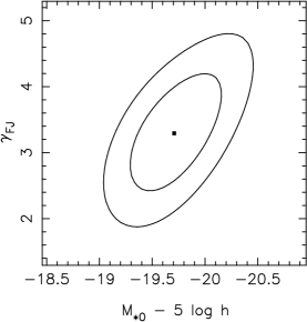
Figure 6: Pairwise constraints for the $B$-band values of $M_{*0}-5\log h$, $\gamma_{FJ}$, and $d\log(M/L)_{B}/dz$ from the Faber-Jackson relation. The contours enclose the $1\sigma$ ($\Delta\chi^{2}<2.30$) and $2\sigma$ ($\Delta\chi^{2}<6.17$) confidence regions.

At rest frame $B$ band, we find a present-day characteristic magnitude of $M_{*0}=-19.70+5\log h\pm 0.29$ (for $\sigma_{DM*}=225\,{\rm km\,s^{-1}}$), a Faber-Jackson slope of $\gamma_{FJ}=3.29\pm 0.58$, and an evolution rate of $d\log(M/L)_{B}/dz=-0.41\pm 0.21$. Fig. 4 shows the input $B$-band magnitudes versus the predicted magnitudes for the best-fit model parameters. The lensing FJ relation forms a coherent correlation over $\sim 4$ mag, with an unweighted rms scatter of $0.53$ mag. We define a normalized luminosity $\log L_{B,norm}=-0.4(M-M_{*0}+1.25\gamma_{FJ}\log\Delta\theta_{red})$ to place all galaxies on a common splitting scale. The effective FJ mass-to-light ratio $\log(M/L)_{B}\equiv-\log L_{B,norm}$ is plotted in Fig. 5. While there is significantly more scatter than in the FP mass-to-light ratios (due to the intrinsically larger scatter of the FJ relation; e.g., Pahre et al. 1998a), a redshift trend is clear. Confidence regions among pairs of fit parameters are plotted in Fig. 6. There are correlations among all three quantities. Of particular interest is the correlation between the evolution rate and FJ slope. This is the result of the increase in the mean $\log\Delta\theta_{red}$ with redshift (Fig. 7). Such a trend is expected from the angular splitting selection function for lenses, as more massive galaxies are needed to produce a fixed angular image separation as the galaxy redshift is increased. However, the absence of low-redshift lens galaxies with large $\log\Delta\theta_{red}$ is puzzling, and this exacerbates the expected trend. It is easy to see how the observed correlation of the mean $\log\Delta\theta_{red}$ with redshift results in correlated values of $d\log(M/L)_{B}/dz$ and $\gamma_{FJ}$. For example, one can make high-redshift galaxies fainter with either a slower evolution rate (so that they are not much brighter than present-day), or a smaller $\gamma_{FJ}$ (so that the luminosity does not increase strongly with the splitting scale, which is characteristically large among high-redshift lenses).

Fits are also performed for the rest frame F555W=$V$, F814W=$I$ and F160W=$H$ bands. The results are summarized in Table 2. Nearly identical values of $\gamma_{FJ}$ are found in all bands, and the evolution rates decrease with increasing wavelength. As with the FP fits in multiple rest frame bands, the estimates are not independent.

The FJ evolution rate is consistent with the FP values, but has a much larger uncertainty. The estimated FJ slope for lenses ($\gamma_{FJ}=3.29\pm 0.58$ at $B$ band) is broadly compatible with recent measurements ($\gamma_{FJ}\simeq 4.0$) in the optical (Forbes & Ponman 1999; Bernardi et al. 2001) and near-infrared (Pahre et al. 1998a). Our scatter of $0.53$ mag about the mean FJ relation is somewhat smaller than found in the above analyses. Still, we must set $\delta_{scale}\gtrsim 2$ for the error bars to reflect the observed scatter, indicating that much of the scatter is intrinsic to the FJ relation. The $B$-band value of $M_{*0}=-19.70+5\log h\pm 0.29$ for gravitational lens galaxies is consistent with luminosity function measurements (e.g., Efstathiou, Ellis & Peterson 1988; Madgwick et al. 2002). Finally, our estimates of $M_{*0}$ and $\gamma_{FJ}$ are consistent with those of Keeton et al. (1998), who performed an FJ analysis on a small sample of gravitational lens galaxies. We note that our error bars on these quantities are larger than they quote, despite our vastly improved galaxy sample. This is easily explained. First, Keeton et al. (1998) used a fixed ($z_{f}=15$) evolutionary model and thus only fit for two parameters. The significant correlations related to the evolution rate imply that constraints on individual parameters will be much weaker when the evolution rate is fit simultaneously. Second, Keeton et al. (1998) individually converted each observed magnitude into a rest frame magnitude, and used all values in the fit. Therefore, a galaxy was represented by a number of data points equal to the number of bands in which it was observed. By over-estimating the degrees of freedom, the uncertainties were under-estimated.

5 Constraints on the Star-formation Redshift

We now constrain the mean star-formation redshift $\langle z_{f}\rangle$ from our sample of 28 gravitational lens galaxies. This may be accomplished in one of two ways. First, we can approximate the predicted evolutionary tracks (Fig. 1) with a linear model ($d\log(M/L)/dz\sim{\rm constant}$), and map the results of §3 and §4 into constraints on $\langle z_{f}\rangle$. Second, we can fit the lens data to the predicted evolutionary tracks directly. Because the linear evolution model becomes a poor approximation for $z_{f}<1.5$, we choose the latter. Note that the derived mean star-formation redshift depends sensitively on the assumed value of the IMF slope (e.g., van Dokkum & Franx 1996), with steeper IMFs leading to lower $\langle z_{f}\rangle$. The IMF is still quite uncertain (e.g., Scalo 1998), so we simply fit to the evolutionary tracks of a Salpeter (1955) IMF to facilitate comparison with other studies. As demonstrated by Treu et al. (2001), changing to a Scalo (1986) IMF has little effect on the derived range for the mean star-formation redshift.

The fits are performed using modified versions of Eq. 5 and 11, in which the linear evolution model is replaced with the detailed evolutionary tracks shown in Fig. 1. Constraints on the typical star-formation redshift are obtained by evaluating $\chi^{2}$ as a function of $\langle z_{f}\rangle$, assuming solar metallicity and an instantaneous starburst. Uncertainties are handled as described in §3 and §4, and the $\chi^{2}$ is renormalized as before. Only $B$-band results are described in detail.

Two trials are performed for the FP evolution. First, we calculate mass-to-light ratio offsets using a fixed local FP intercept (Fig. 8). The best-fit mean star-formation redshift is $\langle z_{f}\rangle=2.1$, and the favored $1\sigma$ ($2\sigma$) range, derived from the $\chi^{2}$ analysis, is $1.9<\langle z_{f}\rangle<2.3$ ($1.8<\langle z_{f}\rangle<2.9$). Second, we allow the local FP intercept to vary, which yields a best-fit of $\langle z_{f}\rangle=2.3$. The increased redshift is consistent with the slightly slower evolution rates found in §3 when the intercept was re-fit. The $1\sigma$ ($2\sigma$) permitted range is $2.0<\langle z_{f}\rangle<3.6$ ($\langle z_{f}\rangle>1.8$). Finally, a similar analysis using the FJ relation yields a $1\sigma$ ($2\sigma$) bound of $\langle z_{f}\rangle>2.6$ ($\langle z_{f}\rangle>1.7$). Constraints on $\langle z_{f}\rangle$ are plotted in Fig. 9. Because the sample of 28 early-type lens galaxies is consistent with old stellar populations, we have little need to invoke significant episodes of secondary star-formation at $z<1$, as suggested by Treu et al. (2001, 2002).

6 Discussion

Gravitational lenses are the only sample of early-type galaxies selected on the basis of mass, rather than luminosity-related properties such as color, magnitude or surface brightness. The lens sample should therefore be much less susceptible to Malmquist bias than luminosity-selected samples, which will tend to over-represent the brightest, bluest and youngest galaxies. Because such selection problems grow more severe at higher redshifts, multi-color imaging surveys are not well suited to extending galaxy samples beyond $z\sim 0.5$, where evolution effects are most pronounced. In contrast, gravitational lensing naturally selects a galaxy sample out to $z\sim 1$, providing a long lever-arm with which to trace evolution. Lenses are therefore excellent tools for investigating the evolution of stellar populations in early-type field galaxies.

We have constrained the rate of luminosity evolution in a sample of 28 early-type gravitational lens galaxies spanning the redshift range $0\lesssim z\lesssim 1$. These galaxies are estimated to have a mean stellar velocity dispersion of $226\,{\rm km\,s^{-1}}$ inside the Coma aperture, with a standard deviation of $55\,{\rm km\,s^{-1}}$. We reiterate that all evolution results apply specifically to this mass scale. First we investigated the fundamental plane, comparing the inferred FP intercept for each galaxy with that of the present-day $B$-band FP (Bender et al. 1998). The lens sample implies an evolution rate of $d\log(M/L)_{B}/dz=-0.56\pm 0.04$ ($1\sigma$) in the rest frame $B$ band. By simultaneously fitting both the evolution rate and the present-day FP intercept, we can minimize possible systematic effects related to the assumed FP slopes and our technique for estimating stellar velocity dispersions. These fits yield a slightly slower evolution rate of $d\log(M/L)_{B}/dz=-0.54\pm 0.09$, and a $z=0$ FP intercept of $\gamma_{0}=-8.88-\log(h/0.5)\pm 0.04$. Finally, we investigated evolution using the Faber-Jackson relation of gravitational lens galaxies, which is closely related to corrected aperture mass-to-light ratios. At rest frame $B$ band, we find a present-day characteristic magnitude of $M_{*0}=-19.70+5\log h\pm 0.29$ (for $\sigma_{DM*}=225\,{\rm km\,s^{-1}}$), a Faber-Jackson slope of $\gamma_{FJ}=3.29\pm 0.58$, and an evolution rate of $d\log(M/L)_{B}/dz=-0.41\pm 0.21$. The evolution rates derived from each of the above measurements are consistent, though the FJ relation offers a rather poor tracer of evolution due to its large intrinsic scatter, and the necessity of fitting three parameters.

The luminosity evolution of gravitational lenses suggests that the stellar populations of early-type field galaxies formed at a mean redshift of $\langle z_{f}\rangle>1.8$ ($2\sigma$), assuming a Salpeter IMF and a flat $\Omega_{m}=0.3$ cosmology. Similar conclusions are derived by van Dokkum et al. (2001), who measure an evolution rate of $d\log(M/L)_{B}/dz=-0.59\pm 0.15$ from a luminosity-selected sample of field E/S0s. These FP evolution results are consistent with a number of recent age estimates (Bernardi et al. 1998; Schade et al. 1999; Im et al. 2002) which favor old, passively-evolving stellar populations for early-type galaxies in the field, thereby contradicting semi-analytic galaxy formation models (e.g., Kauffmann 1996; Kauffmann & Charlot 1998). Alternate conclusions have been drawn by Treu et al. (2002), who measure an evolution rate of $d\log(M/L)_{B}/dz=-0.72^{+0.11}_{-0.16}$ among field E/S0s and favor $\langle z_{f}\rangle\sim 1$ (for a Salpeter or Scalo IMF). We have re-analyzed the Treu et al. (2002) sample, in part to check our own software, and confirm their claim of rapid luminosity evolution. Interestingly, we derive an even faster evolution rate from their sample if the local FP intercept is re-fit, rather than fixed. To explain their rapid evolution, Treu et al. (2001, 2002) suggest that the luminosities of early-type field galaxies may be boosted by secondary episodes of star formation at $z<1$. The claim is supported by the detection of significant [OII] emission in 22% of their sample, similar to the findings of Schade et al. (1999) for field ellipticals out to $z\sim 1$. Menanteau, Abraham & Ellis (2001) further argue that internal color variations detected in this galaxy population are consistent with recent star formation. However, evidence for some recently-formed stellar populations does not necessarily imply rapid luminosity evolution. For example, Schade et al. (1999) detect copious [OII] emission, but still measure a slow rate of luminosity evolution out to $z\sim 1$. [OII] emission of various line-width has also been reported in several early-type gravitational lens galaxies (e.g., Myers et al. 1995; Warren et al. 1996; Fassnacht & Cohen 1998; Tonry & Kochanek 2000; Koopmans & Treu 2002a), even though the evolution rate of the lens sample implies a rather high mean star-formation redshift. Consequently, the presence of [OII] emission does not provide a complete explanation for the rapid rate of luminosity evolution derived by Treu et al. (2002). Additional data and analysis will therefore be necessary to determine whether there is a discrepancy among the various samples of intermediate-redshift early-type field galaxies, and if so, to pinpoint its source.

Our estimates for the luminosity evolution rate and mean star-formation epoch of gravitational lens galaxies have neglected the role of progenitor bias (e.g., van Dokkum & Franx 2001). Because early-type galaxies are believed to form via mergers of star-forming disk galaxies, the high-redshift E/S0 sample comprises only a subset of the progenitors of the local sample. To properly constrain the evolution of stellar populations, one should consider all progenitors of present-day early-type galaxies. However, while the above analyses have considered only early-type lenses, we expect that the inclusion of the rare late-type lenses ($\sim 5/70$) would have little effect on the evolution rate derived from our sample. Therefore, the absence of a significant population of smaller separation, blue, star-forming late-type lens galaxies argues against a strong progenitor bias in our estimation of the evolution rate and star-formation redshift for mass-selected early-type galaxies.

While gravitational lens galaxies are selected on the basis of mass, those entering our analysis sample did need to satisfy a “secondary selection” based on luminosity-related properties: the lens galaxies must be bright enough (at least relative to the quasar components) to obtain robust photometry. The effect of the secondary selection is difficult to quantify, but like any luminosity-related selection, it should lead to the preferential inclusion of brighter galaxies at higher redshifts. Residual Malmquist bias may therefore result in a slightly over-estimated evolution rate in our sample. Note, however, that our ability to estimate stellar velocity dispersions should help minimize the role of Malmquist bias. Velocity dispersions are much more likely to be spectroscopically measured for brighter galaxies, due to signal-to-noise constraints. Considering only those lens galaxies with measured (or measurable) velocity dispersions would therefore likely bias the sample toward faster evolution rates. The first two lenses to be analyzed by the LSD survey (MG2016+112 and 0047–2808; KT) hint at this problem, as each of their implied evolution rates is faster than that of the overall lens sample. Still, the LSD survey will make a significant contribution to evolution studies, particularly via its precision tests of the isothermal hypothesis.

There is much work to be done in order to obtain a complete evolutionary picture of the early-type galaxy population. One obvious improvement would be larger samples of field E/S0s out to intermediate redshift. Unfortunately, the early-type galaxy sample from the Sloan Digital Sky Survey (Bernardi et al. 2001) is rather shallow ($z<0.3$). The SDSS Luminous Red Galaxy Survey (e.g., Eisenstein et al. 2001) aims to select a sample out to $z\sim 0.5$, which should be more appropriate for evolution studies. This will be complemented by the DEEP2 (Davis et al. 2001) galaxy samples at $z>0.7$. Gravitational lenses will continue to play an important role due to their unique status as the only mass-selected galaxies, and newly discovered lenses provide raw material for expanding the current sample. The primary obstacle will be obtaining the necessary HST photometry and ground-based spectroscopy to turn these lenses into viable astrophysical tools. Recent progress on these fronts has, unfortunately, not been commensurate with the discovery rate.

Vastly improved lens samples may one day allow us to pursue more sophisticated analyses of luminosity evolution, such as its dependence on velocity dispersion or color. Studies of environmental dependence will be much more limited, however, as there are very few lenses like Q0957+561, which reside in higher-density environments. Hence, we are unlikely to produce a sample of mass-selected cluster galaxies comparable to our current field sample. More promising are the clues that gravitational lensing may offer regarding the morphological history of field galaxies, for which present knowledge is still rather limited (e.g., Im et al. 1999, 2002). If some high velocity dispersion E/S0s are formed from the mergers of small velocity dispersion disk galaxies at $z<1$, this could potentially be traced directly by the fraction of late-type lenses at different redshifts, or indirectly by the redshift dependence of the mean image separation (Mao & Kochanek 1994; Rix et al. 1994). The current data do not suggest any obvious trends, but the number of spiral lenses is small because they are very inefficient deflectors (e.g., Kochanek 1996). Significantly larger samples of lenses will therefore be needed to fully investigate the relationship between the luminosity and morphological evolution of early-type galaxies in the field.

Appendix A The Faber-Jackson Relation in Observed Bands

Galaxy emission complicates gravitational lens surveys conducted at optical or near-infrared wavelengths (e.g., Kochanek 1993a). To properly interpret observed lensing rates, one must understand the effect of galaxies on both the selection function and completeness. A recent example of this involves calculations of the lensing rate among color-selected high-redshift quasars in the Sloan Digital Sky Survey (Wyithe & Loeb 2002). If a foreground galaxy is multiply-imaging a background quasar, the galaxy emission will affect the derived colors. Hence, a bright lens galaxy can prevent a high-redshift lensed quasar from meeting the color selection criteria. Such biases must be removed by estimating the flux that a lensing galaxy will contribute to a gravitational lens system of a given image separation. This is best accomplished by applying the optical properties of a known sample of gravitational lens galaxies.

We now provide a simple database for estimating the magnitude of an early-type lensing galaxy in a wide range of filters. This is done by determining the correlation among the redshift, the reduced image separation, and the effective absolute magnitude of lensing galaxies in observed bands: $M_{obs}=m_{obs}-DM$, where $DM$ is the distance modulus. The combined effects of evolution and spectral K-corrections are modeled using a single parameter $\gamma_{E+K}$, such that the predicted magnitude is

$$M_{mod}=M_{*0}+2.5\gamma_{E+K}z_{d}-1.25\gamma_{FJ}\log\Delta\theta_{red}\ .$$ (A1)

The fitting function is identical to Eq. 11. If the lens galaxy has not been observed in a given filter, its magnitude is estimated from the available filters using the spectrophotometric model (§2.2). If data are available in that filter, the observed magnitude is used directly. The fit parameters are presented in Table 3 for six HST filters. Despite our crude parameterization of redshift effects, the rms scatters in the relations are, on average, only slightly larger than those in the rest frame bands.

Table 1: Lens Galaxy Photometric Data

Lens	$z_{d}$	$z_{s}$	$E_{Gal}$	$\Delta\theta$	$\log\Delta\theta_{red}$	$\log(r_{e}/^{\prime\prime})$	Filter	Mag
			(mag)	(′′)
0047–2808	0.49	3.60	0.016	2.70	$+0.101$	$-0.04\pm 0.04$	F555W	$20.65\pm 0.05$
							F814W	$18.92\pm 0.27$
Q0142–100	0.49	2.72	0.032	2.24	$+0.045$	$-0.29\pm 0.02$	F160W	$16.63\pm 0.03$
							F814W	$18.72\pm 0.05$
							F675W	$19.35\pm 0.01$
							F555W	$20.81\pm 0.02$
CTQ414	0.28	1.29	0.015	1.22	$-0.238$	$-0.18\pm 0.06$	F160W	$16.67\pm 0.15$
	$\pm 0.02$				$\pm 0.017$		F814W	$18.91\pm 0.37$
							F555W	$20.36\pm 0.18$
MG0414+0534	0.96	2.64	0.303	2.38	$+0.246$	$-0.11\pm 0.08$	F160W	$17.54\pm 0.14$
							F205W	$16.70\pm 0.12$
							F110W	$19.21\pm 0.03$
							F814W	$20.91\pm 0.05$
							F675W	$22.58\pm 0.13$
							F555W	$24.17\pm 0.15$
B0712+472	0.41	1.34	0.113	1.42	$-0.096$	$-0.44\pm 0.06$	F160W	$17.16\pm 0.15$
							F814W	$19.56\pm 0.07$
							F555W	$21.75\pm 0.10$
HS0818+1227	0.39	3.12	0.031	2.83	$+0.102$	$-0.05\pm 0.01$	F814W	$18.76\pm 0.02$
							F555W	$20.78\pm 0.10$
FBQ0951+2635	0.20	1.24	0.022	1.11	$-0.315$	$-0.78\pm 0.11$	F160W	$17.86\pm 0.23$
	$\pm 0.02$				$\pm 0.012$		F814W	$19.67\pm 0.23$
							F555W	$21.02\pm 0.20$
BRI0952–0115	0.38	4.50	0.063	1.00	$-0.371$	$-1.00\pm 0.12$	F160W	$18.95\pm 0.16$
	$\pm 0.03$				$\pm 0.008$		F814W	$21.21\pm 0.04$
							F675W	$22.08\pm 0.03$
							F555W	$23.67\pm 0.08$
LBQS1009–0252	0.78	2.74	0.034	1.54	$-0.039$	$-0.75\pm 0.06$	F160W	$19.30\pm 0.12$
	$\pm 0.10$				$\pm 0.032$		F814W	$21.99\pm 0.04$
							F555W	$24.05\pm 0.25$
Q1017–207	0.86	2.55	0.046	0.85	$-0.217$	$-0.52\pm 0.01$	F160W	$19.26\pm 0.06$
	$\pm 0.15$				$\pm 0.048$		F814W	$21.82\pm 0.48$
							F555W	$25.48\pm 0.73$
FSC10214+4724	0.96	2.29	0.012	1.59	$+0.091$	$+0.06\pm 0.19$	F814W	$20.40\pm 0.39$
	$\pm 0.10$				$\pm 0.044$		F205W	$17.04\pm 0.40$
							F110W	$19.29\pm 0.37$
							F555W	$23.18\pm 0.62$
B1030+074	0.60	1.54	0.022	1.56	$+0.028$	$-0.35\pm 0.06$	F814W	$20.24\pm 0.13$
							F160W	$17.64\pm 0.15$
							F555W	$22.71\pm 0.12$
HE1104–1805	0.73	2.32	0.056	3.19	$+0.309$	$-0.20\pm 0.13$	F160W	$17.47\pm 0.27$
							F814W	$20.01\pm 0.10$
							F555W	$23.14\pm 0.58$
PG1115+080	0.31	1.72	0.041	2.29	$+0.026$	$-0.33\pm 0.02$	F160W	$16.66\pm 0.04$
							F814W	$18.92\pm 0.02$
							F555W	$20.74\pm 0.04$
MG1131+0456	0.84	–	0.036	2.10	$+0.214$	$-0.24\pm 0.05$	F160W	$18.62\pm 0.08$
					$\pm 0.127$		F814W	$21.21\pm 0.04$
							F675W	$22.47\pm 0.06$
							F555W	$23.85\pm 0.24$
HST14113+5211	0.46	2.81	0.016	1.72	$-0.083$	$-0.33\pm 0.05$	F702W	$20.50\pm 0.06$
							F814W	$19.99\pm 0.03$
							F555W	$22.19\pm 0.06$
HST14176+5226	0.81	3.40	0.007	2.84	$+0.225$	$-0.15\pm 0.05$	F160W	$17.53\pm 0.11$
							F814W	$19.77\pm 0.06$
							F606W	$21.91\pm 0.06$
B1422+231	0.34	3.62	0.048	1.56	$-0.177$	$-0.50\pm 0.13$	F160W	$17.57\pm 0.20$
							F791W	$19.66\pm 0.25$
							F555W	$21.80\pm 0.17$
SBS1520+530	0.72	1.86	0.016	1.59	$+0.047$	$-0.46\pm 0.04$	F160W	$17.84\pm 0.06$
							F814W	$20.16\pm 0.13$
							F555W	$21.96\pm 1.24$
MG1549+3047	0.11	–	0.029	2.30	$-0.061$	$-0.09\pm 0.04$	F160W	$14.73\pm 0.07$
					$\pm 0.009$		F205W	$14.00\pm 0.01$
							F814W	$16.70\pm 0.02$
							F555W	$18.19\pm 0.02$
B1608+656	0.63	1.39	0.031	2.27	$+0.242$	$-0.19\pm 0.07$	F160W	$16.76\pm 0.13$
							F814W	$19.02\pm 0.13$
							F555W	$21.24\pm 0.23$
MG1654+1346	0.25	1.74	0.061	2.10	$-0.039$	$-0.05\pm 0.01$	F160W	$15.83\pm 0.04$
							F814W	$17.90\pm 0.02$
							F675W	$18.55\pm 0.01$
							F555W	$19.72\pm 0.03$
B1938+666	0.88	–	0.121	1.00	$-0.088$	$-0.16\pm 0.04$	F160W	$18.67\pm 0.08$
					$\pm 0.154$		F814W	$21.46\pm 0.08$
							F555W	$24.45\pm 0.84$
MG2016+112	1.00	3.27	0.235	3.26	$+0.354$	$-0.66\pm 0.05$	F160W	$18.46\pm 0.09$
							F814W	$21.95\pm 0.09$
							F555W	$25.12\pm 1.06$
B2045+265	0.87	1.28a	0.232	2.28	$+0.265$	$-0.42\pm 0.14$	F160W	$18.25\pm 0.26$
					$\pm 0.145$		F814W	$21.25\pm 0.19$
							F555W	$23.86\pm 0.22$
HE2149–2745	0.50	2.03	0.032	1.70	$-0.039$	$-0.30\pm 0.04$	F160W	$17.61\pm 0.10$
							F814W	$19.56\pm 0.03$
							F555W	$21.18\pm 0.09$
Q2237+030	0.04	1.69	0.071	1.76	$-0.202$	$+0.59\pm 0.08$	F160W	$12.22\pm 0.22$
							F205W	$11.88\pm 0.13$
							F814W	$14.15\pm 0.20$
							F675W	$14.66\pm 0.23$
							F555W	$15.49\pm 0.22$
B2319+051	0.62	–	0.064	1.36	$-0.080$	$-0.65\pm 0.01$	F160W	$18.20\pm 0.02$
					$\pm 0.076$		F814W	$20.71\pm 0.77$
							F555W	$23.43\pm 0.04$

Note. — Listed for each lens are the galaxy ($z_{d}$) and source ($z_{s}$) redshifts, Galactic extinction ($E_{Gal}\equiv E(B-V)$) from Schlegel et al. (1998), standard image separation ($\Delta\theta$), reduced image separation ($\log\Delta\theta_{red}$), intermediate axis effective radius ($\log(r_{e}/^{\prime\prime})$), and magnitudes in each filter. The first filter listed has the highest signal-to-noise ratio, and the surface brightness ($\mu_{e}$) and effective radius are simultaneously fit using a de Vaucouleurs profile. The effective radius is then held fixed when determining $\mu_{e}$ in the remaining filters. The listed magnitudes are extrapolated from the fit quantities, $m=\mu_{e}-5\log r_{e}-2.5\log 2\pi$, and their errors reflect the fitting technique used in each filter. Magnitudes have not been corrected for Galactic extinction in this table, but an $R_{V}=3.1$ extinction curve is used to correct the magnitudes in all calculations and figures. The values of $\log\Delta\theta_{red}$ are calculated assuming $\Omega_{M}=0.3$, $\Omega_{\Lambda}=0.7$. Galaxy redshift errors indicate lenses on which the FP redshift estimation technique has been applied (§2.4). For lenses with unmeasured galaxy or source redshifts, errors on $\log\Delta\theta_{red}$ are constructed using Monte Carlo methods (§2.5). If $z_{d}$ is estimated, correlation between $z_{d}$ and $\log\Delta\theta_{red}$ is important, but here we list the errors obtained by assuming uncorrelated quantities. ^a The B2045+265 (Fassnacht et al. 1999) source redshift is currently disputed, as it implies an uncomfortably large velocity dispersion for the lens galaxy. We therefore treat it as an unknown, and set $z_{s}=2.0\pm 1.0$ as we have done for lenses with unmeasured source redshifts.

Table 2: Evolution Estimates from the Faber-Jackson Relation

Rest Band	$M_{*0}-5\log h$	$\gamma_{FJ}$	$\gamma_{EV}$	rms
$B$	$-19.70\pm 0.29$	$3.29\pm 0.58$	$-0.41\pm 0.21$	0.53
F555W = $V$	$-20.67\pm 0.29$	$3.29\pm 0.58$	$-0.36\pm 0.21$	0.53
F814W = $I$	$-21.86\pm 0.29$	$3.30\pm 0.59$	$-0.31\pm 0.21$	0.53
F160W = $H$	$-23.74\pm 0.29$	$3.34\pm 0.60$	$-0.21\pm 0.22$	0.53

Note. — Listed for each rest frame band are the characteristic magnitude at $z=0$ ($M_{*0}-5\log h$), FJ slope ($\gamma_{FJ}$), evolution rate ($\gamma_{EV}\equiv d\log(M/L)/dz$), and unweighted rms scatter about the best-fit relation.

Table 3: Predicting Observed Lens Galaxy Magnitudes from the Faber-Jackson Relation

Obs Band	$M_{*0}-5\log h$	$\gamma_{FJ}$	$\gamma_{E+K}$	rms
F555W = $V$	$-20.75\pm 0.37$	$3.13\pm 0.83$	$+0.84\pm 0.28$	0.63
F675W = $R$	$-21.86\pm 0.30$	$3.43\pm 0.65$	$+0.73\pm 0.22$	0.56
F814W = $I$	$-21.98\pm 0.30$	$3.21\pm 0.65$	$+0.16\pm 0.23$	0.54
F110W = $J$	$-22.75\pm 0.28$	$3.32\pm 0.57$	$-0.12\pm 0.20$	0.51
F160W = $H$	$-23.79\pm 0.28$	$3.39\pm 0.57$	$-0.21\pm 0.21$	0.52
F205W = $K$	$-24.26\pm 0.27$	$3.32\pm 0.57$	$-0.39\pm 0.20$	0.52

Note. — Listed for each observed band are the characteristic magnitude at $z=0$ ($M_{*0}-5\log h$), FJ slope ($\gamma_{FJ}$), combined evolution plus K-correction parameter ($\gamma_{E+K}$), and unweighted rms scatter about the best-fit relation.

Figure 1: Pure luminosity evolution at rest frame $B$ band. Plotted is the change in $\log(M/L)_{B}$ from its present-day value. The stellar populations have solar metallicity and were formed in an instantaneous burst. A Salpeter IMF is assumed. Tracks are computed with the GISSEL96 version of the Bruzual & Charlot (1993) spectral evolution models, assuming a flat $\Omega_{m}=0.3$ cosmology and $h=0.65$. The predicted evolutionary tracks for star-formation redshifts of $z_{f}=15.0$, $3.0$, $1.5$ and $1.0$ are displayed. Note that later star-formation redshifts result in faster evolution rates. For $z_{f}>1.5$, the evolution rate at $z<1$ can be parameterized as linear in redshift.

Figure 2: Evolution of lens galaxies from the FP at rest frame $B$ band. Plotted is the offset in $\log(M/L)_{B}$ derived using the offset from the local FP intercept of $\gamma_{0}=-8.895-\log(h/0.5)\pm 0.01$. FP slopes of $\alpha=1.25$ and $\beta=0.32$ are assumed. Lenses with known galaxy ($z_{d}$) and source ($z_{s}$) redshifts are plotted as filled squares. Lenses with known $z_{d}$ and assumed $z_{s}=2.0\pm 1.0$ are plotted as open squares. Lenses with estimated $z_{d}$ and known $z_{s}$ are plotted as open circles. Vertical and horizontal error bars are correlated. The solid line depicts the best-fit slope of $d\log(M/L)_{B}/dz=-0.56\pm 0.04$ when $\gamma_{0}$ is fixed. The dashed line depicts the best-fit slope of $d\log(M/L)_{B}/dz=-0.54\pm 0.09$ when $\gamma_{0}$ is simultaneously re-fit.

Figure 3: Simultaneous constraints on the evolution rate and present-day FP intercept $\gamma_{0}$ at rest frame $B$ band. The FP slopes are fixed at $\alpha=1.25$ and $\beta=0.32$. The contours enclose the $1\sigma$ ($\Delta\chi^{2}<2.30$) and $2\sigma$ ($\Delta\chi^{2}<6.17$) confidence regions. The horizontal dashed line represents the local (Coma cluster) FP intercept of $-8.895-\log(h/0.5)$.

Figure 4: The Faber-Jackson relation for gravitational lenses. Plotted is the $B$-band galaxy magnitude versus the prediction of the best-fit model. Lenses with different redshift information are marked as in Fig. 2.

Figure 5: Evolution of the effective Faber-Jackson $B$-band mass-to-light ratio. The scale is arbitrary. The best-fit slope is $d\log(M/L)_{B}/dz=-0.41\pm 0.21$. Lenses with different redshift information are marked as in Fig. 2.

Figure 7: The reduced image separation $\log\Delta\theta_{red}$ as a function of redshift. Dotted lines correspond to constant angular image separations for a source at $z_{s}=2.0$ (bottom to top: $\Delta\theta=0\farcs 5$, $1\farcs 0$, $2\farcs 0$). Lenses with different redshift information are marked as in Fig. 2. The absence of low redshift lens galaxies with large $\log\Delta\theta_{red}$ is puzzling.

Figure 8: Direct fits to evolutionary tracks for a Salpeter IMF. Results are shown for $B$-band FP mass-to-light ratios calculated using a fixed local intercept. Therefore, the plotted data points are identical to those in Fig. 2. An instantaneous starburst and solar metallicity are assumed. Dotted lines represent star-formation redshifts of $z_{f}=15.0$, $3.0$, $1.5$ and $1.0$ (top to bottom). The solid line represents the best-fit track of $\langle z_{f}\rangle=2.1$.

Figure 9: Constraints on the mean star-formation redshift $\langle z_{f}\rangle$ for a Salpeter IMF. Plotted is the renormalized $\Delta\chi^{2}$ as a function of $\langle z_{f}\rangle$. The solid (dashed) line is derived from the FP analysis in which the $z=0$ intercept $\gamma_{0}$ is held fixed (simultaneously re-fit). The dotted line is derived from the FJ analysis. A mean star-formation redshift of $\langle z_{f}\rangle>1.8$ is favored at $2\sigma$ confidence.

References

- (1)
- (2) Bade, N., Siebert, J., Lopez, S., Voges, W., & Reimers, D. 1997, A&A, 317L, 13
- (3)
- (4) Baugh, C.M., Cole, S., & Frenk, C.S. 1996, MNRAS, 283, 1361
- (5)
- (6) Bender, R., Saglia, R.P., Ziegler, B., Belloni, P., Greggio, L., Hopp, U., & Bruzual, G. 1998, ApJ, 493, 529
- (7)
- (8) Bernardi, M., Renzini, A., da Costa, L.N., Wegner, G., Alonso, M.V., Pellegrini, P.S., Rité, C., & Willmer, C.N.A. 1998, ApJL, 508, L143
- (9)
- (10) Bernardi, M., et al. 2001, AJ, submitted (astro-ph/0110344)
- (11)
- (12) Binney, J., & Tremaine, S. 1987, Galactic Dynamics (Princeton: University Press)
- (13)
- (14) Bower, R.G., Lucey, J.R., & Ellis, R.S. 1992, MNRAS, 254, 601
- (15)
- (16) Bruzual, A.G., & Charlot, S. 1993, ApJ, 405, 538
- (17)
- (18) Cardelli, J.A., Clayton, G.C., & Mathis, J.S. 1989, ApJ, 345, 245
- (19)
- (20) Cohn, J.D., Kochanek, C.S., McLeod, B.A., & Keeton, C.R. 2001, ApJ, 554, 1216
- (21)
- (22) Cole, S., Aragon-Salamanca, A., Frenk, C.S., Navarro, J.F., & Zepf, S.E. 1994, MNRAS, 271, 781
- (23)
- (24) Couch, W.J., Barger, A.J., Smail, I., Ellis, R.S., & Sharples, R.M. 1998, ApJ, 497, 188
- (25)
- (26) Davis, M., Efstathiou, G., Frenk, C.S., & White, S.D.M. 1985, ApJ, 292, 371
- (27)
- (28) Davis, M., Newman, J.A., Faber, S.M., & Phillips, A.C. 2001, in Proc. of the ESO/ECF/STScI Workshop on Deep Fields, eds. S. Cristiani, A. Renzini & R.E. Williams (Springer), 241
- (29)
- (30) de Vaucouleurs, G. 1961, ApJS, 5, 233
- (31)
- (32) Djorgovski, S.G., & Davis, M. 1987, ApJ, 313, 59
- (33)
- (34) Dressler, A., Lynden-Bell, D., Burstein, D., Davies, R.J., Faber, S.M., Terlevich, R.J., & Wegner, G. 1987, ApJ, 313, 42
- (35)
- (36) Dressler, A., Oemler, A., Jr., Sparks, W.B., & Lucas, R.A. 1994, ApJL, 435, L23
- (37)
- (38) Dressler, A., et al. 1997, ApJ, 490, 577
- (39)
- (40) Efstathiou, G., Ellis, R.S., & Peterson, B.A. 1988, MNRAS, 232, 431
- (41)
- (42) Eisenstein, D.J., et al. 2001, AJ, 122, 2267
- (43)
- (44) Ellis, R.S., Smail, I., Dressler, A., Couch, W.J., Oemler, A., Jr., Butcher, H., & Sharples, R.M. 1997, ApJ, 483, 582
- (45)
- (46) Fabbiano, G. 1989, ARA&A, 27, 87
- (47)
- (48) Faber, S.M. 1973, ApJ, 179, 731
- (49)
- (50) Faber, S.M., & Jackson, R.E. 1976, ApJ, 204, 668
- (51)
- (52) Fabricant, D., Franx, M., & van Dokkum, P.G. 2000, ApJ, 539, 577
- (53)
- (54) Fassnacht, C.D., & Cohen, J.G. 1998, AJ, 115, 377
- (55)
- (56) Fassnacht, C.D., et al. 1999, AJ, 117, 658
- (57)
- (58) Ferreras, I., Charlot, S., & Silk, J. 1999, ApJ, 521, 81
- (59)
- (60) Foltz, C.B., Hewett, P.C., Webster, R.L., & Lewis, G.F. 1992, ApJL, 386, L43
- (61)
- (62) Forbes, D.A., & Ponman, T.J. 1999, MNRAS, 309, 623
- (63)
- (64) Gerhard, O., Kronawitter, A., Saglia, R.P., & Bender, R. 2001, AJ, 121, 1936
- (65)
- (66) Hagen, H.-J., & Reimers, D. 2000, A&A, 357L, 29
- (67)
- (68) Hernquist, L. 1990, ApJ, 356, 359
- (69)
- (70) Holtzman, J.A., Burrows, C.J., Casertano, S., Hester, J.J.; Trauger, J.T., Watson, A.M., & Worthey, G. 1995, PASP, 107, 1065
- (71)
- (72) Huchra, J., Gorenstein, M., Kent, S., Shapiro, I., Smith, G., Horine, E., & Perley, R. 1985, AJ, 90, 691
- (73)
- (74) Im, M., Griffiths, R.E., Naim, A., Ratnatunga, K.U., Roche, N., Green, R.F., & Sarajedini, V.L. 1999, ApJ, 510, 82
- (75)
- (76) Im, M., et al. 2002, ApJ, 571, 136
- (77)
- (78) Jorgensen, I., Franx, M., & Kjaergaard, P. 1996, MNRAS, 280, 167
- (79)
- (80) Jorgensen, I., Franx, M., Hjorth, J., & van Dokkum, P.G. 1999, MNRAS, 308, 833
- (81)
- (82) Kauffmann, G., White, S.D.M., & Guiderdoni, B. 1993, MNRAS, 264, 201
- (83)
- (84) Kauffmann, G. 1996, MNRAS, 281, 487
- (85)
- (86) Kauffmann, G., & Charlot, S. 1998, MNRAS, 294, 705
- (87)
- (88) Keeton, C.R., Kochanek, C.S., & Falco, E.E. 1998, ApJ, 509, 561
- (89)
- (90) Keeton, C.R., Christlein, D., & Zabludoff, A.I. 2000, ApJ, 545, 129
- (91)
- (92) Kelson, D.D., van Dokkum, P.G., Franx, M., Illingworth, G.D., & Fabricant, D. 1997, ApJL, 478, L13
- (93)
- (94) Kelson, D.D., Illingworth, G.D., van Dokkum, P.G., & Franx, M. 2000, ApJ, 531, 184
- (95)
- (96) Kochanek, C.S. 1993a, ApJ, 417, 438
- (97)
- (98) Kochanek, C.S. 1993b, ApJ, 419, 12
- (99)
- (100) Kochanek, C.S. 1994, ApJ, 436, 56
- (101)
- (102) Kochanek, C.S. 1995, ApJ, 445, 559
- (103)
- (104) Kochanek, C.S. 1996, ApJ, 466, 638
- (105)
- (106) Kochanek, C.S., et al. 2000, ApJ, 543, 131
- (107)
- (108) Koopmans, L.V.E., et al. 1999, MNRAS, 303, 727
- (109)
- (110) Koopmans, L.V.E., & Treu, T. 2002a, ApJL, 568, L5
- (111)
- (112) Koopmans, L.V.E., & Treu, T. 2000b, ApJ, in press (astro-ph/0205281)
- (113)
- (114) Lavery, R.J., & Henry, J.P. 1988, ApJ, 330, 596
- (115)
- (116) Lawrence, C.R., Schneider, D.P., Schmidet, M., Bennett, C.L., Hewitt, J.N., Burke, B.F., Turner, E.L., & Gunn, J.E. 1984, Sci, 223, 46
- (117)
- (118) Lehár, J., Cooke, A.J., Lawrence, C.R., Silber, A.D., & Langston, G.I. 1996, AJ, 111, 1812
- (119)
- (120) Lehár, J., et al. 2000, ApJ, 536, 584
- (121)
- (122) Lilly, S.J., Tresse, L., Hammer, F., Crampton, D., & Le Fevre, O. 1995, ApJ, 455, 108
- (123)
- (124) Lin, H., Yee, H.K.C., Carlberg, R.G., Morris, S.L., Sawicki, M., Patton, D.R., Wirth, G., & Shepherd, C.W. 1999, ApJ, 518, 533
- (125)
- (126) Lubin, L.M., Fassnacht, C.D., Readhead, A.C.S., Blandford, R.D., & Kundic, T. 2000, AJ, 119, 451
- (127)
- (128) Lucey, J.R., Bower, R.G., & Ellis, R.S. 1991, MNRAS, 249, 755
- (129)
- (130) Madau, P., Pozzetti, L., & Dickinson, M. 1998, ApJ, 498, 106
- (131)
- (132) Madgwick, D.S., et al. 2002, MNRAS, 333, 133
- (133)
- (134) Mao, S.D., & Kochanek, C.S. 1994, MNRAS, 268, 569
- (135)
- (136) Menanteau, F., Abraham, R.G., & Ellis, R.S. 2001, MNRAS, 322, 1
- (137)
- (138) Morgan, N.D., Dressler, A., Maza, J., Schechter, P.L., & Winn, J.N. 1999, AJ, 118, 1444
- (139)
- (140) Myers, S.T. et al. 1995, ApJL, 447, L5
- (141)
- (142) Muñoz, J.A., Kochanek, C.S., & Keeton, C.R. 2001, ApJ, 558, 657
- (143)
- (144) Pahre, M.A., Djorgovski, S.G., & de Carvalho, R.R. 1998a, AJ, 116, 1591
- (145)
- (146) Pahre, M.A., de Carvalho, R.R., & Djorgovski, S.G. 1998b, AJ, 116, 1606
- (147)
- (148) Pahre, M.A., Djorgovski, S.G., & de Carvalho, R.R. 2001, Ap&SS, 276, 983
- (149)
- (150) Press, W.H., Teukolsky, S.A., Vetterling, W.T., & Flannery, B.P. 1992, Numerical Recipes (Cambridge: University Press)
- (151)
- (152) Ratnatunga, K.U., Ostrander, E.J., Griffiths, R.E., & Im, M. 1995, ApJL, 453, L5
- (153)
- (154) Rix, H.-W., Maoz, D., Turner, E.L., & Fukugita, M. 1994, ApJ, 435, 49
- (155)
- (156) Rix, H.-W., de Zeeuw, P.T., Cretton, N., van der Marel, R.P., & Carollo, C.M. 1997, ApJ, 488, 702
- (157)
- (158) Rusin, D., Norbury, M., Biggs, A.D., Marlow, D.R., Jackson, N.J., Browne, I.W.A., Wilkinson, P.N., & Myers, S.T. 2002, MNRAS, 330, 205
- (159)
- (160) Salpeter, E. 1955, ApJ, 121, 161
- (161)
- (162) Scalo, J. 1986, Fund. Cosmic Phys., 11, 1
- (163)
- (164) Scalo, J. 1998, in ASP Conf. Ser. 142, The Stellar Initial Mass Function: 38th Herstmonceux Conf., ed. G. Gilmore & D. Howell (San Francisco: ASP), 201
- (165)
- (166) Schade, D., et al. 1999, ApJ, 525, 31
- (167)
- (168) Schlegel, D.J., Finkbeiner, D.P., & Davis, M. 1998, ApJ, 500, 525
- (169)
- (170) Schneider, P., Ehlers, J., & Falco, E.E. 1992, Gravitational Lenses (Berlin: Springer-Verlag)
- (171)
- (172) Scodeggio, M., Gavazzi, G., Belsole, E., Pierini, D., & Boseilli, A. 1998, MNRAS, 301, 1001
- (173)
- (174) Scodeggio, M. 2001, AJ, 121, 2413
- (175)
- (176) Stanford, S.A., Eisenhardt, P.R., & Dickinson, M. 1998, ApJ, 492, 461
- (177)
- (178) Tonry, J.L. 1998, AJ, 115, 1
- (179)
- (180) Tonry, J.L., & Kochanek, C.S. 1999, AJ, 117, 2034
- (181)
- (182) Tonry, J.L., & Kochanek, C.S. 2000, AJ, 119, 1078
- (183)
- (184) Trager, S.C., Faber, S.M., Worthey, G., & González, J.J. 2000, AJ, 119, 1645
- (185)
- (186) Treu, T., Stiavelli, M., Bertin, G., Casertano, S., & Moller, P. 2001, MNRAS, 326, 237
- (187)
- (188) Treu. T., Stiavelli, M., Casertano, S., Moller, P., & Bertin, G. 2002, ApJL, 564, L13
- (189)
- (190) Treu, T., & Koopmans, L.V.E. 2002a, ApJ, 575, 87
- (191)
- (192) Treu, T., & Koopmans, L.V.E. 2002b, MNRAS, 337L, 6
- (193)
- (194) Turner, E.L., Ostriker, J.P., & Gott, J.R., III 1984, ApJ, 284, 1
- (195)
- (196) van Dokkum, P.G., & Franx, M. 1996, MNRAS, 281, 985
- (197)
- (198) van Dokkum, P.G., Franx, M., Kelson, D.D., & Illingworth, G.D. 1998, ApJL, 504, L17
- (199)
- (200) van Dokkum, P.G., Franx, M., Fabricant, D., Kelson, D.D., & Illingworth, G.D. 1999, ApJL, 520, L95
- (201)
- (202) van Dokkum, P.G., Franx, M., Fabricant, D., Illingworth, G.D., & Kelson, D.D. 2000, ApJ, 541, 95
- (203)
- (204) van Dokkum, P.G., & Franx, M. 2001, ApJ, 553, 90
- (205)
- (206) van Dokkum, P.G., Franx, M., Kelson, D.D., & Illingworth, G.D. 2001, ApJL, 553, L39
- (207)
- (208) Vogt, N.P., Forbes, D.A., Phillips, A.C., Gronwall, C., Faber, S.M., Illingworth, G.D., & Koo, D.C. 1996, ApJL, 465, L15
- (209)
- (210) Walsh, D., Carswell, R.F., & Weymann, R.J. 1979, Nature, 279, 381
- (211)
- (212) Warren, S.J., Hewett, P.C., Lewis, G.F., Moller, P., Iovino, A., & Shaver, P.A. 1996, MNRAS, 278, 139
- (213)
- (214) White, S.D.M., & Rees, M.J. 1978, MNRAS, 183, 341
- (215)
- (216) Worthey, G. 1994, ApJS, 95, 107
- (217)
- (218) Wyithe, J.S.B., & Loeb, A. 2002, ApJ, 577 57
- (219)
- (220) Ziegler, B.L., et al. 2002, ApJL, 564, L69
- (221)