Uncertainties in Spiral Galaxy Projection Parameters

Abstract

We investigate the impact of nonaxisymmetric structure on estimates of galaxy inclinations and position angles. A new minimization technique is used to obtain estimates of inclination and position angle from a global fit to either photometric or kinematic data. We discuss possible systematic uncertainties which are much larger than statistical uncertainties. Our investigation reveals that systematic uncertainties associated with fitting photometric data dominate the formal statistical uncertainties. For our sample of inclined galaxies, we estimate that nonaxisymmetric features introduce inclination and position angle uncertainties of $\approx 5^{\circ}$, on average. The magnitudes of these uncertainties weaken the arguments for intrinsically elliptical galaxy disks.

1 Introduction

We observe disk galaxies projected at random angles on the sky and must, therefore, determine the inclination geometry for each galaxy in order to deproject line-of-sight velocity data, or discover the intrinsic shape of the disk, etc. The in-plane orbital speed is needed for mass estimation, and is also one of the parameters required for the Tully-Fisher relation (hereafter TFR, Tully & Fisher 1977). Furthermore, correction for internal extinction is also inclination-dependent (e.g., Giovanelli et al. 1994), affecting the total luminosity of the galaxy, the other parameter of the TFR. Thus errors in both the inclination and position angle, propagate directly into dynamical mass estimates, luminosity estimates, and contribute to the scatter in systematic relations.

The most common procedure to determine orientation geometry is to fit ellipses to a photometric image of the galaxy, and to infer the projection geometry by assuming the disk to be intrinsically thin and axisymmetric. The ellipticity of the projected image, $\epsilon=1-b/a$ where $b$ and $a$ are respectively the semi-minor and semi-major axis lengths, is related to the inclination angle through $\cos{i}=1-\epsilon$, for an assumed intrinsically axisymmetric, infinitesimally thin, disk. Here, $i$ is the inclination angle of the disk plane to the plane of the sky ($i=0^{\circ}$ for a face-on galaxy), and we use the symbol $\phi$ for position angle of the line of intersection of these two planes. A slightly more complicated relation exists for galaxies that are assumed to be thin oblate spheroids (Hubble, 1926).

If 2-D velocity fields are available, they can also be used to determine inclinations and position angles. The previously mentioned assumptions of intrinsic axisymmetry and thinness are again typical. A drawback to this method is that it is poorly suited to determine inclinations where the rotation curve rises slowly (Van Moorsel & Wells, 1985). On the other hand, 2-D velocity fields can clearly delineate position angles.

Garcia-Gomez & Athanassoula (1991) summarize several other procedures that have been adopted to estimate $\epsilon$ from photometry in the presence of the complicating non-axisymmetric features – spirals, bars, lop-sidedness, etc. – manifested by virtually all disk galaxies.

The IRAF utility ellipse implements the method outlined by Jedrzejewski (1987) and fits ellipses to a number of isophotes independently, although the task can be instructed to hold any parameter, such as the photometric center, fixed for all. The formal statistical uncertainties due to noise in the data (hereafter abbreviated to statistical uncertainties) in the fitted parameters are not easily obtained (Busko, 1996), but are generally quite small. The user of this utility then has to make a judgement as to which isophote, or group of isophotes, offers the best estimate of the projection geometry. A common prejudice is that the outer disk is more likely to be intrinsically round, leading to a preference for the outermost, or the average of several outer ellipses. Another strategy is to identify the true shape with a radial range over which the fitted parameters do not vary much.

Such a procedure clearly does not utilize all the information in the image. More sophisticated methods include: minimizing the $m=2$ component of the Fourier transform of an image (Grosbøl, 1985), bulge-disk decomposition (Kent, 1985), maximizing the $m=0$ component of deprojected images (Iye et al., 1982), and fitting a parametric model for the disk (Palunas & Williams, 2000). We propose another global method which, like those just cited, assumes that the galaxy disk is infinitesimally thin and intrinsically axisymmetric. Our method returns $\epsilon$ and $\phi$ values from a chi-squared minimization using a large part of the image. The details are summarized in the Appendix.

The statistical uncertainty of the methods described above is usually small, but it is clear that the possible systematic error could be large if the disk is intrinsically non-circular or if nonaxisymmetric features are present. In this paper, we attempt to quantify the possible systematic error from a detailed re-analysis of the photometric and 2-D kinematic maps of a sample of 74 spiral galaxies already reported by (Palunas & Williams, 2000) (hereafter PW).

After briefly introducing the data sets used in the study in §2, we give a general discussion (§3) of the statistical and systematic errors that can arise when estimating projection angles. In §4, we present the results of photometric and kinematic fitting procedures applied to the PW galaxies. Unlike these authors, however, we study possible systematic errors in estimating the projection parameters by comparing our fits to the kinematic and photometric data.

2 Data

We have used the disk fitting methods described in the Appendix to estimate the projection angles, $i$ and $\phi$, from the $I$-band photometry and 2-D velocity fields for the 74 galaxies in the PW sample. PW kindly provided the reduced photometric images with the foreground stars removed.

PW also determined 2-D velocity fields for the same galaxies from H$\alpha$ spectroscopy taken with the Rutgers Fabry-Perot imaging spectrophotometer. They obtained several (8 to 15) images spaced by 1 Å($\approx 50$ km/s at H$\alpha$) of each galaxy from which they derived data cubes ($x,y,v_{los}$). These cubes were then reduced to 2D spatial maps by fitting the line profiles at each pixel with a Voigt function. Again, PW kindly supplied us with the resulting velocity fields, H$\alpha$ intensities, continuum intensities, and their respective uncertainties.

Inclined galaxies were preferred in this sample, which is therefore notably deficient in nearly face-on systems. This selection bias makes our study complementary to those by Rix & Zaritsky (1995) and Anderson et al. (2001) who focused on face-on systems.

3 Statistical & Systematic Uncertainties

Noise in the data (photometric or kinematic) creates statistical parameter uncertainties, $\sigma_{x}$, which can be measured in a variety of ways. For example, the curvature of the reduced chi-squared, $\chi^{2}_{r}$ , surface at the minimum, $\chi^{2}_{r}=\chi^{2}_{r,{\rm min}}$, or better, the distance from the minimum at which $\chi^{2}_{r}=\chi^{2}_{r,{\rm min}}+\Delta\chi^{2}_{r}$, allows estimates of the statistical uncertainies in the parameters, and any covariances. Confidence limits can be determined from the contours at $\Delta\chi^{2}_{r}=n/\nu$, where $\nu$ is the number of degrees of freedom, i.e., the number of pixels minus the number of free parameters in the fit, and $n$ is an integer. Clearly, the magnitudes of the statistical uncertainties in the estimated parameters are small when many pixels are used, and statistical uncertainties in the projection angles frequently turn out to be $\ll 1^{\circ}$.

Sources of systematic uncertainties, $s_{x}$, in photometric ellipse fitting include: (1) seeing, (2) dust obscuration, (3) finite disk thickness, (4) non-axisymmetric features in the disk, and (5) intrinsic ellipticity of the disk. Velocity field fitting is also subject to similar systematics. Points 4 and 5 are relevant to both methods. Additionally, if a nearly edge-on galaxy with finite thickness has rotational velocities that decrease with height away from the midplane, fitting a thin disk model leads to an apparent inclination that is somewhat less edge-on than in reality.

Seeing tends to bias elliptical isophotes towards becoming round. While it is most severe in the central regions, the effect can be of the same order as an intrinsic ellipticity for moderate distances from the center (Trujillo et al., 2001). Using the typical seeing value quoted in PW of $1^{\prime\prime}.5$ and Figure 1 of Trujillo et al. (2001), we find that at a radius 12 times the seeing length a measured $\epsilon$ value is $\approx 90\%$ of its actual value. This can lead to errors in $i$ of a few degrees, depending on the value of $i$. However, since most of the pixels utilized to make the fits lie beyond 12 times the seeing length (and are less affected by seeing), the effect is probably less important than others we discuss below.

Since inclined galaxies suffer more extinction than do face-on galaxies, dust is a source of systematic error. Its effect can be reduced by utilizing photometry in near IR bands where dust extinction is less severe, as we do in this study.

Using simulation and analytical work, we have found that photometrically determined $i$ values are significantly affected by finite thickness only for the most edge-on galaxies (inclination $\gtrsim 80^{\circ}$). Photometric fits of model inclined oblate spheroids agree well with the formula given in Hubble (1926) relating inclination, apparent axis ratio, and spheroidal axis ratio. Since the majority of the PW galaxies have $i\leq 80^{\circ}$, we ignore this complication hereafter.

Nonaxisymmetric structures in disks, such as bars, spirals, and warps, are a major source of systematic error. Stock (1955) investigated the impact of spiral structure on the photometric estimation of position angles, particularly the case of highly inclined galaxies, finding that spiral structure can introduce uncertainties in $\phi$ values of $\approx 5^{\circ}$. We refer to the impact of all such nonaxisymmetric structure on the photometric projection angles as the spiral effect.

Several studies, most notably Binney & de Vaucouleurs (1981); Grosbøl (1985); Franx & de Zeeuw (1992); Rix & Zaritsky (1995); Beauvais & Bothun (1999); Anderson et al. (2001), have found hints that the disks of spirals are not perfectly axisymmetric, which may arise because the gravitational potential well within which the disk material orbits is intrinsically non-axisymmetric. We distinguish this global intrinsic oval distortion of the disk from more obvious features in the disk, such as spiral arms and bars. One reason for drawing this distinction is that the spiral effect can be investigated using photometric data only, while the effects of intrinsic ellipticity should be most clear when photometric data are compared to kinematic data (Franx & de Zeeuw, 1992). Depending on how the major axis of an elliptic disk is projected, an intrinsic ellipticity can lead to either larger or smaller inferred ellipticity values, leading to over- or under-estimates of the inclination, and to corresponding errors in the position angle.

4 Results

PW determined the projection angles for each galaxy separately from the photometric and kinematic data. In general, they found somewhat different values from the two methods, which was inconvenient for their objective. They wished to compare the observed rotation curve with that predicted from a photometric disk mass model, which requires a common projection geometry for both. They argued that the inclination and position of the geometric center could be determined most reliably from the photometry, while the position angle of the major axis was best determined from the kinematics. They then re-fitted both data sets with the preferred parameter from the other set held fixed.

Our inclinations derived from photometry are in good agreement with the values reported in PW. While reassuring, the agreement is scarcely surprising as we are using similar methods to fit the same photometric data. Discrepancies arise, in part, because we have fitted for both $i$ and $\phi$ while in PW $\phi$ was held fixed at the value determined from the kinematics, but the good agreement (the average difference between our $i_{\rm phot}$ values and those of PW is $2.9^{\circ}$ shows that this constraint has a small effect. The largest difference is $19^{\circ}$ and occurs for ESO 510G11, a galaxy with very strong spirals that extend into the outer parts of the disk.

One of our principal objectives here is to understand the discrepancy between the photometric and kinematic values of the projection angles for each galaxy. The magnitudes of these differences are illustrated in Figures 1a and 1b. The statistical uncertainties are much smaller than the symbols in both figures.

The inclinations show considerable spread around perfect agreement (Figure 1a). The average photometric/kinematic inclination difference is $\approx 5^{\circ}$ with a standard deviation of similar magnitude. A comparison of position angles (Figure 1b) shows a similar spread, with one extreme outlier which we discuss briefly below. The average difference between position angle estimates is $\approx 4^{\circ}$ (excluding the extreme outlier). Note, however, that this galaxy sample is deficient in nearly face-on galaxies and that Anderson et al. (2001) found larger differences in a sample of 10 low inclination ($i\lesssim 20^{\circ}$) galaxies.

Figures 2a and 2b show the relations between the inclination and position angle differences and the photometric inclination of the galaxy. While there is significant spread in Figure 2b, there appears to be a trend for more highly inclined galaxies to have smaller position angle differences. Such a trend is expected, since any nonaxisymmetric structures present in highly-inclined galaxies should have only a small effect on $\phi_{\rm phot}$. This trend also agrees with the aforementioned larger differences found for low inclination galaxies (Anderson et al., 2001).

The largest position angle difference in Figure 2b corresponds to a galaxy which has a low inclination and strong spirals which extend to the outer reaches of the disk. It is a prime example of the kind of systematic error that can be attributed to the spiral effect. Additionally, this kind of misalignment could cause serious problems if single-slit spectroscopic data were to be utilized to determine rotation curves. Misalignment between the slit and the true major axis results in an underestimate of rotational speed and hence dynamical mass.

4.1 Fixed Centers vs. Floating Centers

In all the work reported elsewhere in this paper, we have required the rotation center of our fitted model to coincide with the peak of continuum brightness in the image (see Appendix). In this subsection, we report the consequences of relaxing this requirement and determine the kinematic center from the velocity field alone. The offset between the kinematic and photometric centers, and the resulting differences in estimates for $i$ and $\phi$ are illustrated in Figure 3.

Figure 3a shows that the kinematic center is $\lesssim 2.\arcsec 7$ from the photometric center in the majority (67 of 74) of galaxies. The galaxy for which this distance is largest, ESO 322G42, has a slowly rising rotation curve, which creates nearly parallel isovelocity contours; the location of the center and the overall systemic velocity are poorly constrained by such data, but the inner slope of the rotation curve is independent of the center location. Six other galaxies are in the tail ($\Delta r_{\rm cen}>2.\arcsec 7$): One (ESO 445G19) has a strongly asymmetric inner velocity field, while the others are either nearly edge-on and have roughly parallel isovels and slowly rising rotation curves, or lack H$\alpha$ emission near the center; the location of the rotation center is not tightly constrained in the absence of kinematic information near the center.

As evidenced by the histograms in Figures 3b and c, the projection angles that result from fitting with the kinematic center free to move agree with those from the fixed-center fits for the majority of the galaxies. In fact, none of the $\phi$ values changes by more than $4^{\circ}$. The changes in inclination show a larger range, but 70 of 74 galaxies have $\Delta i<7^{\circ}$. The galaxy with the largest $\Delta i$ shows evidence of being tidally distorted, having a long filament of anomalous velocities extending from its edge. The two galaxies with the next largest $\Delta i$ values both have strong spirals resulting in velocity fields with strong distortions. The remaining galaxy in the tail of the $\Delta i$ histogram is a highly inclined galaxy that is also in the tail of the $\Delta r_{\rm cen}$ histogram.

We find that unless the kinematic center is poorly constrained by a slowly rising rotation curve, it lies within $\approx 2.\arcsec 5$ of the position of the photometric center for most galaxies. So, if rotation curves of our galaxy sample were determined from single-slit spectra taken through the point of maximum continuum, they would not be significantly biased towards rising slowly. Allowing a small shift in the kinematic center generally makes little difference to the estimated projection angles, except in a few special cases.

4.2 Spiral Effect Systematics

In an attempt to estimate the magnitude of the uncertainties due to the spiral effect, we have proceeded as follows. (Note that these values must be viewed as lower limits to the true systematics, which are unknown.) We use a first estimate of the photometric projection parameters from our $\chi^{2}_{r}$ minimization procedure to deproject a galaxy image. We then rotate it through an angle $\beta$, so that the nonaxisymmetric structure lies in a new orientation, and then reproject it to the original best-fit $i$ and $\phi$. We then apply our photometric fitting apparatus to this new image to find new best-fit $i$ and $\phi$ values. We interpret the spread in both $i$ and $\phi$ as $\beta$ varies through a half-rotation as the measures of systematic uncertainties $s_{i}$ and $s_{\phi}$ due to the presence of nonaxisymmetric features in the image. A few representative plots of $i$ and $\phi$ versus $\beta$ are presented in the next section.

The results of this investigation are shown in Figure 4. Galaxies that have $i\gtrsim 75^{\circ}$ have been excluded from this analysis because deprojection must be considered suspect for such large inclination angles. The general trend of decreasing $s_{i}$ and $s_{\phi}$ with increasing $i$ concurs with our earlier assertion that nonaxisymmetric structure should compromise the model fits more modestly for highly inclined galaxies. The galaxy with the highest values of $s_{i}$ and $s_{\phi}$ (ESO 323G39) appears to have a significant bar.

The numbers in Figure 4 denote different galaxy $T$-types, where low numbers indicate early-type spirals and high numbers indicate late-type spirals and irregulars. The different $T$-types do not nicely segregate in either frame of Figure 4. However, there is a statistical trend for later type galaxies to have larger $s_{i}$ and $s_{\phi}$ values. Early type spirals ($T$-types 0-3) have average $s_{i}$ values of $\approx 3^{\circ}$ and average $s_{\phi}$ values of $\approx 4^{\circ}$. Spirals with $T$-types between 4 and 6 have average $s_{i}\approx 4^{\circ}$ and $s_{\phi}\approx 4^{\circ}$. Late type spirals ($T$-types $\geq 7$) have average $s_{i}\approx 6^{\circ}$ and $s_{\phi}\approx 7^{\circ}$. The differences between the means of the early and intermediate spirals are not statistically significant. However, the differences between the early and late types’ means are significant at the 95% level. For all galaxies with $i<75^{\circ}$, the average $s_{i}\approx 4^{\circ}$ and $s_{\phi}\approx 5^{\circ}$, with a large spread for both values. The magnitudes of $s_{i}$ and $s_{\phi}$ suggest that the uncertainties in $i$ and $\phi$ values derived from photometry are dominated by systematic uncertainty due to nonaxisymmetric structure.

4.3 Intrinsic Ellipticities vs. the Spiral Effect

We find differences between the projection angles determined by fitting photometric and kinematic data. Franx & de Zeeuw (1992), Anderson et al. (2001), and others suggest that such disagreements are evidence of intrinsically elliptical disks, but such a conclusion requires that the projection angles can be determined with sufficient precision for their differences to have meaning.

Our investigation of the spiral effect points to significant systematic errors in the photometric determination of projection angles which are of the same magnitude as the errors suggested by Franx & de Zeeuw (1992) to explain the scatter in the TFR. This leads us to wonder whether differences between photometric and kinematic projection angles are evidence of anything more than our ignorance of the true angles.

Fortunately, we can use our 2D velocity fields to search for evidence of intrinsic ellipticity. Franx, van Gorkom, & de Zeeuw (1994) formulate elliptical orbits in disks in the epicyclic approximation with a small $m=2$ forcing term added to the central attaction. This distortion is entirely contained within the plane of the disk. For the special case of a flat rotation curve, the distortions in the radial and tangential directions are equal and can be described by,

$$v_{\rm R}=v_{\rm circ}\epsilon_{\rm int}\sin{2(\psi-\gamma)},$$ (1a)

and

$$v_{\phi}=v_{\rm circ}[1+\epsilon_{\rm int}\cos{2(\psi-\gamma)}].$$ (1b)

Here $v_{\rm circ}$ is the circular speed, $\epsilon_{\rm int}$ is the intrinsic ellipticity of the disk, $\psi$ is the angle in the disk measured from the projected major axis, and $\gamma$ is the angle between the projected major axis and the elliptical disk minor axis. When such a disk is inclined, the line-of-sight velocity field appears as that of an axisymmetric disk with small correction terms added,

$$v_{\rm los,ellip}=$$ (2)

$$v_{\rm los,axisym}-$$

$$\epsilon_{\rm int}v_{\rm circ}\sin{i}(\cos{2\gamma}\cos{\psi}-\sin{2\gamma}\sin{\psi}),$$

where $v_{\rm los,axisym}$ is the line-of-sight velocity for an axisymmetric disk with the same projection angles. Equation 2 demonstrates that a mildly elliptical disk creates an $m=1$ distortion in the residual velocity field, at a position angle which depends on $\gamma$. (There is also an $m=3$ term in the more general case of a non-flat rotation curve, see Franx, van Gorkom, & de Zeeuw 1994 for details.)

In order to quantify the strength of such distortions, we introduce two quantities, $P$ and $Q$ which we derive from the velocity residuals in the following way. We divide the residual field inside the outermost fitting ellipse into 15 elliptical annuli, and divide each annulus into quadrants. We label the first quadrant (I) to be that bounded by the receding side of the projected major axis and the minor axis counter-clockwise from it, and the remaining quadrants (II, III, IV) are in the usual order. For each quadrant in each annulus, we calculate the average of the residuals $\bar{r}_{n,{\rm quad}}$, normalized by the average of the magnitude of the residuals in the entire field. We then define $P$ and $Q$ values for each annulus as follows,

$$P=|\bar{r}_{n,{\rm I}}+\bar{r}_{n,{\rm II}}-\bar{r}_{n,{\rm III}}+\bar{r}_{n,{\rm IV}}|$$ (3a)

and

$$Q=|\bar{r}_{n,{\rm I}}+\bar{r}_{n,{\rm IV}}-\bar{r}_{n,{\rm II}}+\bar{r}_{n,{\rm III}}|.$$ (3b)

Basically, $P$ measures the strength of an $m=1$ distortion across the major axis, while $Q$ measures the same thing across the minor axis. Plotting $A\equiv\sqrt{P^{2}+Q^{2}}$ values versus the semi-major axis of the annulus provides an asymmetry profile.

Using equation 2, we have constructed a model residual velocity field for a disk with nested similar concentric elliptical orbits. The resulting asymmetry profile rises rapidly in the central region of the residual field, but then flattens and remains constant for the remaining radial range. None of the galaxies we have studied show this kind of asymmetry profile. Galaxies which have bars and/or strong spirals show peaks in their asymmetry profiles (for example, Figures 5c VI and 5d VI), but the distortion is localized and not seen throughout the entire disk. It is also interesting to note that a higher-than-average level of asymmetry in a velocity field is not always associated with a significant difference between photometric and kinematic projection angles.

5 Individual Galaxies

Here we present several individual galaxies that illustrate the difficulty of measuring accurate projection angles. For each galaxy, we show an $I$-band image, a 2D velocity field, a residual photometric image, a residual velocity field, a plot illustrating the spiral effect, and an asymmetry profile. The photometric images are presented in grayscales with units of magnitudes per arcsecond squared. The white circles in the photometric images mark the locations of stars that have been removed. In the photometric residual images, the central white circles mask the pixels that are associated with a bulge and/or bar and are therefore not included in the fits. The velocity fields are given in units of kilometers per second. The velocity and residual velocity fields display the pixels with measurement uncertainties less than 25 km/s. The suppressed pixels do not strongly influence the fitted parameters. The spiral effect plot is composed of one frame showing the response of the fitted $i$ value to the rotation of the image and another showing how $\phi$ changes with the rotation. In the asymmetry profiles, asterisks mark the $A$ values for the residual velocity fields.

Since photometric data is often more extensive than kinematic data, some of the images in the following figures may appear unequal. As described in the Appendix, the data used by our fitting routine is different for photometric and kinematic fits. However, we utilize the maximum amount of information in both cases. To test the impact of the differing radial extents of the data, we fit the photometric data over the same radial range as the kinematic data. There were no significant changes in the average differences between photometric and kinematic inclinations or position angles. For the remainder of the paper, the results given are derived using the maximum amount of information for the data set.

5.1 ESO 439G20 & ESO 322G45

The photometric images of ESO 439G20 (Figure 5a I) and ESO 322G45 (Figure 5b I) appear to be free of strong bars and spiral structure. Their respective velocity fields also appear to be those of simple inclined axisymmetric disks (Figures 5a II and 5b II). The naive assumption is that these two “nice” galaxies should show little asymmetry and should have good agreement between their photometric and kinematic projection angles.

For ESO 439G20, the photometric and kinematic $i$ difference is $3.5^{\circ}$ and the $\phi$ difference is $1.6^{\circ}$. The lack of strong nonaxisymmetric structure is evident from the photometric residual (Figure 5a III) and the plot illustrating the spiral effect (Figure 5a V). The asymmetry profile (Figure 5a VI) shows little influence of bars or spirals. The last $A$ value is due to the small blue and red spots on either side of the minor axis on the right side of Figure 5a IV.

ESO 322G45 has an $i$ difference of $4.7^{\circ}$ and a $\phi$ difference of $4.5^{\circ}$. Figures 5b III and 5b V are evidence that there is little asymmetry in the photometric image. Again, the asymmetry profile (Figure 5b VI) is fairly featureless. The last two $A$ values may be the effect of a weak spiral arm that appears in the photometric residual image $\approx 20$ arcsec from the center. It is surprising that such a featureless galaxy has large $i$ and $\phi$ differences, but they cannot be symptoms of intrinsic ellipticity in the disk, for the following reasons: An elliptical disk viewed in projection should generally give rise to the type of asymmetry profile discussed in §4.3, which is not seen in Fig. 5b VI. The special case of projection about one of the disk’s principal axes could mask this signature, but then we should not expect a significant $\Delta\phi$, which we also find. Thus, we are confident that the differences in this case are not due to an intrinsically elliptic disk.

These two galaxies serve to illustrate the point that just because a galaxy’s image or velocity field appears smooth or simple does not imply accurate estimation of projection angles.

5.2 ESO 267G29 & ESO 569G17

In contrast to the previous examples, we present two galaxies whose photometric images (Figures 5c I and 5d I) show strong bars and spiral structure. Their velocity fields (Figures 5c II and 5d II) contain distorted isovelocity contours, evidence of strong nonaxisymmetric structure. In these cases, it is not unreasonable to believe that estimation of projection angles will be problematic.

ESO 267G29 has a photometric/kinematic $i$ difference of $20^{\circ}$ and a $\phi$ difference of $15^{\circ}$. The strong open spiral can be clearly seen in Figure 5c III and the effect of the central bar is obvious from the $m=1$ residual pattern in central region of Figure 5c IV. The asymmetry profile (Figure 5c VI) clearly shows the effect of the central bar with the rise in $A$ at large radius due most likely to the strong spiral also present.

To again contrast, the differences between photometric and kinematic $i$ and $\phi$ values for ESO 569G17 are $<1^{\circ}$. A dusty multi-armed spiral pattern can be seen in Figure 5d III. As before, the effect of the central bar is evident in the residual velocities (Figure 5d IV). Like ESO 267G29, the asymmetry profile in Figure 5d VI shows the impact of a central bar and some effect from spiral arms.

It is not surprising that if the central region of the velocity field of ESO 267G29 is ignored, as it is in the photometry, the differences between photometric and kinematic $i$ and $\phi$ drop to $\approx 10^{\circ}$. In contrast, ignoring the central region of the velocity field of ESO 569G17 increases the discrepancy between photometric and kinematic projection angles by $\approx 1^{\circ}$. So, even though photometric images and kinematic maps are complicated, the projection angles derived from them can be consistent. These two examples also suggest that the details of the spiral structure present can significantly alter the photometric/kinematic discrepancy.

5.3 ESO 215G39

As our final example, we present a “typical” spiral galaxy. The photometric/kinematic $i$ difference is $1.9^{\circ}$ and the $\phi$ difference is $2.3^{\circ}$. The photometry and residuals (Figures 5e I and 5e II) show moderate spiral structure and the velocity field (Figure 5e II) is fairly simple. The velocity residual field (Figure 5e IV) shows some evidence of elliptical orbits in the central region. Again, the asymmetry profile (Figure 5e VI) contains evidence of either a weak central bar or spirals near the center. Interestingly, the magnitudes of these photometric/kinematic differences are the same as the predicted differences due to the spiral effect for this galaxy.

6 Discussion & Conclusions

We have developed and tested a global fitting method with a novel minimization technique to obtain disk galaxy inclinations and position angles from either photometric or kinematic data. Since we fit a thin axisymmetric disk model to all the data at once, we determine globally optimal values for the geometric parameters, $\epsilon$ and $\phi$. This contrasts with the IRAF ellipse utility which returns independent $\epsilon$ and $\phi$ values for each of many ellipses, and cannot be constrained to find the best common values.

We map the $\chi^{2}_{r}$ surface to find the best-fit inclination and position angle and to determine the statistical uncertainty for each fit. Due to the large number of data points (typically $\gtrsim 10^{3}$), the statistical uncertainty is very small. The $i$ and $\phi$ values determined using our method differ only slightly from those previously estimated for the same 74 spiral galaxies by Palunas & Williams (2000). While we have held the rotation center fixed at the location of brightest continuum, changes in derived quantities are generally small when we allow the kinematic center to move from this point.

A major result of this study is that systematics dominate photometrically determined inclination and position angle uncertainties. We estimate that systematic uncertainties due to nonaxisymmetric structure such as spirals and/or bars are, on average, $\approx 4^{\circ}$ for inclination estimates and $\approx 5^{\circ}$ for position angle estimates for galaxies in this sample. Again, we point out that the complete systematic error is unknown, and these estimates must be taken as lower limits. It is reassuring that the position angle uncertainties tend to be smaller for more edge-on galaxies and that later type spirals generally have larger systematic inclination and position angle uncertainties. It seems that the only way to reduce these systematic errors would be to model the nonaxisymmetric structure in each galaxy.

It is interesting to note that the average difference in inclination and position angle derived from the photometric and kinematic data turn out to be roughly the same size as our estimates for uncertainties due to nonaxisymmetric structure. Since these differences are also similar to those expected from intrinsically elliptical disks, they reinforce the concern raised by Franx & de Zeeuw (1992) and Rix & Zaritsky (1995) that spiral structure can be confused with intrinsic disk ellipticity. As discussed in §5, the (non)existence of spirals and/or bars does not necessarily imply (small) large differences between photometric and kinematic projection angles. We also find no clear evidence for the velocity field distortions expected for intrinsically elliptic disks.

To conclude, we have found a difference between galaxy projection angles determined from photometric and kinematic data for 74 galaxies. We have also found that nonaxisymmetric structures, such as spirals and bars, impact the galaxies’ photometric projection angles to about the same extent as the differences between photometric and kinematic projection angles. Further, we see no direct evidence for intrinisically elliptical disks in any of our galaxies’ residual velocity fields. In light of these points, it seems unnecessary to explain photometric/kinematic projection angle differences with intrinsic disk ellipticities.

Appendix A Procedure to Estimate Projection Angles

The principle of our method is to use as much information as possible from a photometric or kinematic image to estimate the two angles of projection. If a galaxy were a razor-thin, axisymmetric disk and the orbits were circular, then the surface brightness or in-plane orbital speed would be constant on a nested set of concentric, co-axial, similar ellipses. We utilize the entire velocity field, from the center of the galaxy to beyond its edge, but our photometric fits are to only those parts of the image not strongly contaminated by bulge and/or bar components.

Our input data are a set of data values $\{D_{i}\}$, and their associated uncertainties, $\{\sigma_{i}\}$, for each of the $N$ pixels in the image. For photometric data, on the one hand, the $\{D_{i}\}$ are pixel intensity values, for which the principal source of noise is photon counting. We estimate the sky brightness from part of the image away from the galaxy and subtract its value before beginning the fit. For kinematic data, on the other hand, the $\{D_{i}\}$ are line-of-sight velocity values and the associated uncertainties result from the fitting of the Fabry-Perot data cube.

We choose the center to have the coordinates $(x_{c},y_{c})$ of the pixel that has the largest intensity for a photometric image, or the largest continuum intensity for the velocity map. We generally hold these coordinates fixed for the entire fitting procedure, although our method can allow the center to move if desired.

We fit a non-parametric profile that is characterized by a tabulated set of values $\{M_{k}\}$, for a number $K$ of semi-major axes. Each $M_{k}$ has the same value around an ellipse, and all ellipses have a common center and ellipticity, $\epsilon$, and major-axis position angle, $\phi$, embodying our assumption that the disk is thin and axisymmetric. For photometric data, the $\{M_{k}\}$ are isophote intensities, while they are circular velocities for a kinematic map. Note such a tabular form makes no assmuption about the radial profile of either the light or the orbital speed. We derive a model prediction at a general location in the image by finding the semi-major axis of the ellipse that passes through the point in question, and then interpolate for the predicted pixel value from the $\{M_{k}\}$.

For any values of the projection parameters ($\epsilon,\phi$), we form

$$\chi^{2}_{r}=\frac{1}{\nu}\sum^{N}_{i=1}\left[\frac{D_{i}-\sum^{K}_{k=1}w_{k,i}M_{k}}{\sigma_{i}}\right]^{2},$$ (A1)

where the $w_{k,i}$ are the weight factors that describe the interpolation scheme, and $\nu$ is the number of degrees of freedom in the fit. Since $\chi^{2}_{r}$ is linear in the $M_{k}$s, the $M_{k}$s that minimize $\chi^{2}_{r}$ can be determined by setting the derivative of eq. (A1) with respect to each $M_{j}$ equal to zero and solving the resulting set simultaneous equations,

$$\sum^{K}_{k=1}\left(\sum^{N}_{i=1}\frac{w_{j,i}}{\sigma_{i}}\frac{w_{k,i}}{\sigma_{i}}\right)M_{k}=\sum^{N}_{i=1}\frac{w_{j,i}}{\sigma^{2}_{i}}D_{i}.$$ (A2)

The resulting $M_{k}$ values are used to determine $\chi^{2}_{r}$ . Our implementation uses linear interpolation to determine the $w_{k,i}$ factors, but more complicated schemes would be straightforward to implement. Any pixels that lie outside the final fitting ellipse have their model values linearly extrapolated from the values of the last two ellipses and their weights smoothly decreased depending on their distance from the last ellipse. Such pixels have little impact on the best-fit parameters.

We use slightly different methods to determine which pixels will be used in the fitting procedure for the photometric and kinematic data. In both cases, we create a pixel list only once which is used throughout the fitting procedure. With photometric data, we exclude pixels contaminated by foreground stars or cosmic rays. We also exclude those pixels inside a circular aperture containing a central bulge or bar, and set the smallest semi-major axis of the $K$ ellipses equal to the radius of this inner aperture. The outer limit of the pixel list is defined by an outer elliptical aperture with semi-major axis 10% larger than that of the outermost fitting ellipse, using an initial estimate of the ellipticity. The pixel list for the kinematic data contains all pixels that have continuum intensity values $\geq 0.5\%$ the central continuum intensity. We add, in quadrature, a fixed velocity dispersion of $7\;$km s^-1 to the estimated velocity uncertainty in the line fit. Some anomalous velocities remain in the velocity map, possibly caused by intervening gas not associated with the galaxy of interest or from Voigt profile fits near the velocity limits of the Fabry-Perot data cube; we eliminate such values by applying a simple cut to exclude pixels with velocities more than 500 km/s away from the data value at the fixed center.

We vary the two projection angles, $\epsilon$ and $\phi$, recomputing the $\{M_{k}\}$ at each iteration to determine their values that minimize $\chi^{2}_{r}$ . We use a downhill simplex method, specifically the amoeba routine described in Press et al. (1992), which requires only $\chi^{2}_{r}$ function evaluations (no derivatives) and initial estimates for $\epsilon$ and $\phi$. Following the recommendation of Press et al. (1992), the $\epsilon$ and $\phi$ estimates returned are re-used as initial guesses for up to 5 subsequent calls to amoeba to converge to the $\chi^{2}_{r}$ minimum. We have verified the minimum location by inspecting the $\chi^{2}_{r}$ surface surrounding the best-fit values. Projections of the contour where $\chi^{2}_{r}=\chi^{2}_{r,{\rm min}}+1.0/\nu$ onto the $\epsilon$ and $\phi$ axes provide 1-$\sigma$ statistical uncertainty measurements.

Figure 6 shows the results of photometric fitting for one galaxy in our sample (ESO 215G39). The model isointensity values are shown as filled circles superimposed on data values. The solid lines encompass 68% of the data values. The statistical uncertainties of the parameters (dot values) are smaller than the symbols. The rotation curve with 1-$\sigma$ parameter uncertainties resulting from the kinematic fit for the same galaxy is shown in Figure 7.

Figure 1: a) Inclinations determined from photometric data ($i_{\rm phot}$) compared with those determined from kinematic data ($i_{\rm vel}$). b) Position angles determined from photometric data ($\phi_{\rm phot}$) compared to those determined from kinematic data ($\phi_{\rm vel}$). The extreme outlier is discussed in the text. The solid lines in both frames are lines of equality.

Figure 2: a) The difference between inclination angles determined from photometric data and kinematic data plotted against the photometric inclination. b) The difference between position angles determined photometrically and kinematically versus the photometric inclination. Note that the $\Delta\phi$ scatter shrinks as the inclination increases. The extreme outlier is discussed in the text.

Figure 3: a) Histogram of the distance between the photometric center and the fitted kinematic center. The difference is $<2.\arcsec 7$ for the majority (90%) of the galaxies. b) Histogram of the change in estimated inclination between the fixed-center and floating-center fits. 95% of the galaxies have $\Delta i<7^{\circ}$. c) Histogram of the change in position angle between the fixed-center and floating-center fits. None of the galaxies has $\Delta\phi>4^{\circ}$.

Figure 4: Systematic uncertainties in (a) photometric inclination, (b) photometric position angle. The numbers denote the $T$-type of the galaxy. Note that the scatter decreases with increasing $i_{\rm phot}$.

Figure 5: (I) $I$-band image of the galaxy. The white circles show the locations of removed foreground stars. The units are ${\rm mag}/{\rm arcsec}^{2}$. (II) The line-of-sight velocity field from Fabry-Perot interferometry. The values listed are heliocentric velocities in km/s. (III) Photometric residuals using the best-fit $i_{\rm phot}$ and $\phi_{\rm phot}$. The units are ${\rm mag}/{\rm arcsec}^{2}$. The ellipse marks the location of the last ellipse used in the fitting routine. The central white circle masks the pixels that are associated with a bulge and/or bar. (IV) The residual velocity field using the best-fit $i_{\rm vel}$ and $\phi_{\rm vel}$. As explained in the text (see §5), only those pixels with measurement uncertainties $<25\;$km/s are shown. (V) The variation of the fitted $i$ and $\phi$ as the image is rotated as described in §4.2 (VI) The radial variation of $A$ to reveal the asymmetry profile. Discussion for each galaxy is given in the text.

Figure 5: Continued

Figure 5: Continued

Figure 5: Continued

Figure 5: Continued

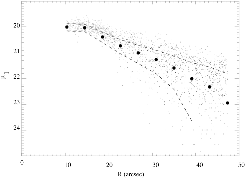
Figure 6: Model isophote values $\{M_{k}\}$ (filled circles) versus semi-major axis for the galaxy ESO 215g39. Some indicative (but not all) sky-subtracted data values are plotted. The dashed lines contain 68% of the data values and the 1-$\sigma$ uncertainties for the model values are much smaller than the filled circles.

Figure 7: Estimated rotation curve for the galaxy ESO 215g39. The crosses with error bars are the $\{M_{k}\}$ values returned from the kinematic fitting routine together with their 1-$\sigma$ statistical uncertainties.

References

- Anderson et al. (2001) Anderson, D.R., Bershady, M.A., Sparke, L.S., Gallagher, J.S., & Wilcots, E.M. 2001, ApJ, 551, 131
- Beauvais & Bothun (1999) Beauvais, C. & Bothun G. 1999, ApJS, 125, 99
- Binney & de Vaucouleurs (1981) Binney, J.J. & de Vaucouleurs, G. 1981, MNRAS, 194,679
- Busko (1996) Busko, I. 1996, in Proceedings of the Fifth Astronomical Data Analysis Software and Systems Conference (PASP Conf. Series v.101), ed. G.H. Jacoby and J. Barnes, p. 139-142
- Franx & de Zeeuw (1992) Franx, M. & de Zeew, T. 1992, ApJ, 392, 47
- Franx, van Gorkom, & de Zeeuw (1994) Franx, M., van Gorkom, J.H., & de Zeeuw, T. 1994, ApJ, 436, 642