On the small-scale stability of thermonuclear flames in Type Ia supernovae

Abstract

We present a numerical model which allows us to investigate thermonuclear flames in Type Ia supernova explosions. The model is based on a finite-volume explicit hydrodynamics solver employing PPM. Using the level-set technique combined with in-cell reconstruction and flux-splitting schemes we are able to describe the flame in the discontinuity approximation. We apply our implementation to flame propagation in Chandrasekhar-mass Type Ia supernova models. In particular we concentrate on intermediate scales between the flame width and the Gibson-scale, where the burning front is subject to the Landau-Darrieus instability. We are able to reproduce the theoretical prediction on the growth rates of perturbations in the linear regime and observe the stabilization of the flame in a cellular shape. The increase of the mean burning velocity due to the enlarged flame surface is measured. Results of our simulation are in agreement with semianalytical studies.

1 Introduction

Owing to the vast range of relevant length scales involved in the problem, it is impossible to resolve the full Type Ia supernova (SN Ia in the following) explosion in multidimensional numerical simulations. Therefore the task has to be tackled in different approaches to gain insight to various aspects of the explosion mechanism. Large Scale Calculations (LSCs) try to model the explosion on scales of the stellar radius (for a recent example see Reinecke et al. (2002)). The motivation of our work is to model thermonuclear flames and to analyze the effective velocity of their propagation which is a crucial input for LSCs.

For SN Ia various explosion mechanisms have been suggested (for a review see Hillebrandt & Niemeyer (2000)). We refer to the class of so-called Chandrasekhar mass models in which the C+O white dwarf accretes sufficient amounts of material to reach the Chandrasekhar mass $M_{\mathrm{ch}}$ where carbon burning is initiated. At the prevailing temperatures of typically around $10^{10}\,\mathrm{K}$ the thermonuclear burning is confined to a very narrow region which is called a flame. Numerical simulations indicate that a promising scenario is that the explosion starts out as a deflagration which gets accelerated by turbulence (“pure turbulent deflagration model”), or makes a transition to a detonation later on (“delayed detonation model”). Thus a main ingredient of all deflagration SN Ia models is the acceleration of the burning velocity owing to turbulence generated by instabilities of the flame. The wrinkling of the flame front as a result of turbulent flow extends the surface area of the front and thereby increases its mean propagation rate. On large scales the dominating instability is the Rayleigh-Taylor instability, caused by the stratification of dense fuel and lighter ashes inverse to the gravitational field. Owing to this instability rising bubbles of burning material form, leading to shear (Kelvin-Helmholtz) instabilities on their surfaces. These effects are believed to generate the necessary amount of turbulence to explain the burning velocities required for SN Ia explosions.

Nevertheless it remains crucial for the understanding of SN Ia explosions to investigate the flame evolution on intermediate scales, that is on scales much smaller than the dimension of the exploding star, but still much larger than the inner flame structure. The most important questions in this scale range are: Is the turbulence in SN Ia entirely driven by large-scale effects or can effects on intermediate scales contribute to the increase of the turbulent burning velocity of the flame front? Is there a mechanism to trigger a deflagration-to-detonation transition (DDT) (Ivanova et al., 1974; Khokhlov, 1991; Woosley & Weaver, 1994)? A possible effect that could be the answer to both questions would be the existence of so-called “active turbulent combustion” (Kerstein, 1996; Niemeyer & Woosley, 1997). Therefore interaction of flame instabilities with a turbulent flow field is of particular interest.

Here we report the first step to find an answer to these questions, namely the study of the Landau-Darrieus (LD hereafter) instability in a quiescent flow in two spatial dimensions. The LD instability (Landau, 1944; Darrieus, 1938) acts on propagating density discontinuities such as thin chemical or thermonuclear flame fronts. In the nonlinear regime, this instability is known to give rise to the formation of a cellular structure that stabilizes the front against further growth of perturbations (Zel’dovich, 1966). There is a number of previous publications dealing with this topic, e.g. Gutman & Sivashinsky (1990), Blinnikov & Sasorov (1996), Helenbrook & Law (1999). Our approach is in the spirit of the work by Niemeyer & Hillebrandt (1995) who first demonstrated the existence of the LD instability in thermonuclear burning in white dwarf matter at densities relevant for SN Ia explosions in a numerical simulation. The main difference between their and our approach lies in the flame description. Niemeyer & Hillebrandt (1995) resolve the thermal structure of the flame thereby restricting the spatial scale space that can be investigated numerically. In contrast to their model we describe the flame in a fully parametrized way as a discontinuity making use of level set and in-cell reconstruction/flux-splitting techniques. This method stands in direct succession of Reinecke et al. (1999) and gives us more flexibility in numerical experiments.

2 Flame model

In general, the structure of laminar deflagration flames can be thought of as composed of two zones: the convective diffusive zone where the fuel is preheated (in our case by electron conduction) to reach non-negligible reaction rates and the thin reactive diffusive zone where the reaction actually takes place. This picture sets both the width $d_{l}$ and the propagation velocity $s_{l}$ of the laminar flame with respect to the unburnt matter. A study of laminar flames in the context of thermonuclear burning in degenerate matter by means of direct numerical simulation can be found in Timmes & Woosley (1992).

The burning releases energy and heats the burnt material resulting in an increase of temperature across the flame. In case of thermonuclear burning in white dwarfs the fuel consists of material containing a degenerate electron gas. Since the degeneracy of the relativistic electron gas is partly removed in the burnt matter, the temperature increase across the flame yields a decrease in density. Thus, if the scales under consideration are much larger than the flame width (less than a centimeter for laminar flames in C+O white dwarfs, see Timmes & Woosley (1992)), it is well justified to simplify the flame model to a moving discontinuity in the state variables. This discontinuity approximation does not resolve the inner structure of the flame. It is therefore necessary to prescribe the laminar burning velocity of the front as an additional parameter taken from direct numerical simulations.

Thermonuclear burning in SN Ia is characterized by turbulent combustion and takes place in the so-called flamelet regime for the part of the explosion where most of the energy is released. Here turbulence is driven on large scales by the rising Rayleigh-Taylor bubbles invoking a turbulent cascade. The scaling law of this cascade is still controversial, it may simply follow Kolmogorov-scaling or, as pointed out by Niemeyer & Kerstein (1997), Bolgiano-Obukhov scaling. In any case, the velocity fluctuation $u^{\prime}$ is a function of the scale $l$ and Niemeyer & Kerstein (1997) show that there exists a scale between the size of the largest turbulent eddies and the flame width on which the eddy turnover time becomes comparable to the flame crossing time. Therefore the flame dynamics below that scale is not affected by large-scale fluctuations. In case of chemical flames the cutoff scale is known as Gibson length $l_{\mathrm{gibs}}$.

This defines the range in length scales we address in our intermediate flame structure investigation as

$$d_{l}\ll l\ll l_{\mathrm{gibs}}.$$ (1)

Realistic values for these length scales at a density of $5\times 10^{7}\mathrm{g}\,\mathrm{cm}^{-3}$ are less than $1\,\mathrm{cm}$ for the flame width (Timmes & Woosley, 1992) and about $10^{4}\,\mathrm{cm}$ for the Gibson length according to Niemeyer (1998).

3 The Landau-Darrieus instability

On the intermediate scales defined by (1) the burning front can be described as a laminar flame, which is unaffected by turbulence on large scales and dominated by the LD instability. This instability is caused by the refraction of the streamlines of the flow on the density change over the flame (approximated as a discontinuity). The fluid velocity component tangential to the flame front is steady and mass conservation leads to a discontinuity in the normal velocity component. Consider a flame front that is perturbed from an originally planar shape. Mass flux conservation leads to a broadening of the flow tubes in the vicinity of a bulge of the perturbation. Thus the local fluid velocity is lower than the fluid velocity at $\pm\infty$. Therefore the burning velocity $s_{l}$ of the flame is higher than the corresponding local fluid velocity and this leads to an increment of the bulge. The opposite holds for recesses of the perturbed front. In this way the perturbation keeps growing. By means of a linear stability analysis Landau found for the growth rate of the perturbation amplitude

$$\omega_{\mathrm{LD}}=ks_{l}\frac{\mu}{1+\mu}\left(\sqrt{1+\mu-\frac{1}{\mu}}-1\right),$$ (2)

where $k$ denotes the perturbation wavenumber and $\mu=\rho_{u}/\rho_{b}$ is the density contrast across the flame front.

The LD instability would in principle lead to unlimited growth of small perturbations of the planar flame shape. It has, however, been ignored in all large scale SN Ia models so far because there exists a nonlinear stabilization mechanism which limits the perturbation growth. Following Zel’dovich (1966) this effect can be explained in terms of geometrical considerations: The propagation of an initially sinusoidally perturbed flame is followed by means of Huygens’ principle (see Figure 1).

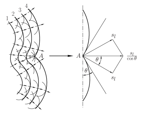
Figure 1: Nonlinear stabilization of the flame front (adapted from Zeldovich et al. (1980)).

After a while a cusp forms at the interfaces of neighboring cells (marked with $A$ in Figure 1). Here Huygens’ principle breaks down and the flame propagation enters the nonlinear regime. The propagation velocity at the cusp exceeds $s_{l}$:

$$u_{\mathrm{cusp}}=\frac{s_{l}}{\cos\theta},$$ (3)

where $\theta$ is the angle between the propagation velocity of the cusp and the normal direction of adjacent cell segments. This leads to a stabilization of the flame in a cellular shape which has been observed in experiments.

An analytical description of the flame propagation in the cellular burning regime has been given by Sivashinsky (1977) and by Frankel (1990). The equations established there have been widely used in the chemical combustion community and were applied to the context of SN Ia by Blinnikov & Sasorov (1996), where a description of the cellular flame front in a fractal model is given. As the authors point out, these approaches to model flame fronts do not allow to answer the question, weather the stabilization can break up under certain conditions (e.g. certain densities; interaction with turbulent velocity fields). In case of a break-up the LD instability would lead to a further increase of the effective burning speed. In this context a transition from the deflagration mode of flame propagation to a detonation (DDT) comes into consideration. A DDT has been successfully implemented into empirical supernova models (Höflich & Khokhlov (1996), Iwamoto et al. (1999)), but the mechanism for it to occur is still unclear (Niemeyer, 1999). Numerical simulations by Niemeyer & Hillebrandt (1995) indicate a break-up of the cellular stabilization and subsequent turbulization of the burning front. One objective of the numerical model presented here is a thorough investigation of this result. This is of great interest because it could provide the mechanism for “active turbulent combustion” (ATC) proposed by Kerstein (1996) and discussed in the context of SN Ia explosions by Niemeyer & Woosley (1997).

In the following section we present a numerical method that will allow us to study the stability of the cellular flame structure.

4 Numerical Methods

Our implementation of the flame model goes back to the methods described in (Reinecke et al., 1999) where details of the numerical implementation can be found. The fluid dynamics is described by the reactive Euler equations. These are discretized on an equidistant cartesian grid and solved by applying the Piecewise Parabolic Method (PPM) suggested by Colella & Woodward (1984) in the PROMETHEUS implementation (Fryxell et al., 1989).

The equation of state applied in our calculations comprises the contributions that describe white dwarf matter. It includes an arbitrarily degenerate and relativistic electron gas, local black body radiation, an ideal gas of nuclei, and electron-positron pair creation/annihilation (see e.g. Cox & Giuli (1968)).

The treatment of the flame in the discontinuity approximation is based the so-called level-set technique that was introduced by Osher & Sethian (1988). The central idea of the level-set method is to associate the flame with a moving hypersurface $\Gamma(t)$ that is the zero level set of a function $G(\mbox{\boldmath{$r$}},t)$:

$$\Gamma(t):=\{\mbox{\boldmath{$r$}}\;|\;G(\mbox{\boldmath{$r$}},t)=0\}.$$ (4)

The function $G$ is prescribed to be a signed distance function

$$|\mbox{\boldmath{$\nabla$}}G|\equiv 1$$ (5)

with respect to the flame front and with $G<0$ in the unburned material and $G>0$ in the ashes. The temporal evolution of $G$ is given by

$$\frac{\partial G}{\partial t}=(\mbox{\boldmath{$v$}}_{u}\mbox{\boldmath{$n$}}+s_{l})|\mbox{\boldmath{$\nabla$}}G|$$ (6)

for points located on the front. $\mbox{\boldmath{$v$}}_{u}$, $n$, and $s_{l}$ denote the fluid velocity in the unburnt region, the normal vector to the flame front, and the burning speed with respect to the unburnt material, respectively.

Our method crucially depends on the particular realization of the coupling between the hydrodynamic flow and the flame which will be reviewed in the following.

4.1 Flame/flow coupling

In the context of the finite-volume method we apply to discretize the hydrodynamics, the cells cut by the flame front (“mixed cells” in the following) contain a mixture of burnt and unburnt states. Therefore the quantity $\mbox{\boldmath{$v$}}_{u}$ needed in (6) is not readily available. One strategy to circumvent this problem is the so-called “passive implementation” of the level-set method as described in Reinecke et al. (1999). There it is assumed that the velocity jump is small compared with the laminar burning velocity and $\mbox{\boldmath{$v$}}_{u}$ is approximated by the average flow velocity. An operator splitting approach for the time evolution of $G$ (6) yields the advection term owing to the fluid velocity in conservative form which is identical to the advection equation of a passive scalar. This part can be treated by the PROMETHEUS implementation of the PPM method. Front propagation, energy release, and species conversion as a result of burning are accomplished in an additional step.

The strategy we use is called “complete implementation” by Reinecke et al. (1999). It was developed by Smiljanovski et al. (1997). In these papers various tests of the numerical method, as for instance the evolution of a spherical flame, are presented. Smiljanovski et al. (1997) also compare with experimental results for chemical flames. Our numerical implementation reproduces the numerical tests successfully and because it does not differ from the previous implementation in substantial points, we will not repeat the tests here.

The special way of flame/flow coupling in the “complete implementation” enables us to reconstruct the exact burnt and unburnt states in mixed cells. This allows exact treatment of (6). The main advantage is that it becomes now possible to treat flows of burnt and unburnt material over cell boundaries separately preventing the flame front from smearing out over several cells as it does for the “passive implementation”. The flame front is resolved as a sharp discontinuity without any mesh refinement that would lead to very small CFL timesteps. The “complete implementation” consisting of in-cell reconstruction and flux-splitting schemes will be reviewed in the following paragraphs. The description is restricted to two-dimensional simulations.

4.1.1 Geometrical information

A prerequisite of the in-cell reconstruction and flux-splitting schemes is the knowledge of geometrical quantities as the front normal $n$, the unburnt volume fraction of mixed cell and the unburnt fraction of the interface area between the cells. The normal vector of the flame front can be directly derived from the $G$ field,

$$\mbox{\boldmath{$n$}}=-\frac{\mbox{\boldmath{$\nabla$}}G}{|\mbox{\boldmath{$\nabla$}}G|},$$ (7)

and is defined to point towards the unburnt material.

The unburnt volume fraction $\alpha$ of a cell is obtained from the intersections of the zero level set of the $G$-function with the cell interfaces. Connecting these intersection points with a straight line results in a piecewise linear approximation of the flame in the cells and $\alpha$ is obtained by calculating the area behind the connecting line. This procedure is depicted in Figure 2.

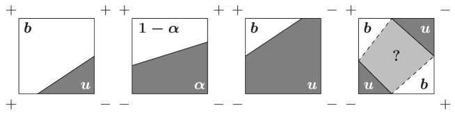
Figure 2: Determination of $\alpha$ in mixed cells. The signs on the cell corners denote the sign of $G$ at these locations (adapted from Reinecke et al. (1999)).

The rightmost sketch shows a situation where the geometry is ambiguous. In these (fortunately rare) cases that $\alpha$ of the two possibilities is taken which is closest to the value of the preceding time step.

4.1.2 In-cell reconstruction and flux-splitting

In order to reconstruct the unburnt and burnt states in mixed cells we set up a system of equations. The first three equations of that reconstruction system of equations describe the cell averages of the conserved quantities as linear combinations of the unburnt and the burnt part of the cell:

$$\overline{\rho} = \alpha\rho_{u}+(1-\alpha)\rho_{b}$$ (8)

$$\overline{\rho\mbox{\boldmath{$v$}}} = \alpha\rho_{u}\mbox{\boldmath{$v$}}_{u}+(1-\alpha)\rho_{b}\mbox{\boldmath{$v$}}_{b}$$ (9)

$$\overline{\rho e} = \alpha\rho_{u}e_{u}+(1-\alpha)\rho_{b}e_{b}$$ (10)

Here, $\rho$ stands for the mass density, $\rho\mbox{\boldmath{$v$}}$ for the momentum density, and $\rho e$ for the density of the total energy. The indices $u$ and $b$ denote the unburnt and burnt quantities respectively.

Continuity of mass flux density, momentum flux density and energy flux density over the flame front yield the Rankine-Hugoniot jump conditions and the Rayleigh criterion. To incorporate the former into the system of equations it is convenient to split the velocity vector into a normal part $\mbox{\boldmath{$v$}}_{n}$ and a tangential part $\mbox{\boldmath{$v$}}_{t}$ with respect to the front. Eq. (9) then reads

$$\overline{\rho v}_{n}=\alpha\rho_{u}v_{n,u}+(1-\alpha)\rho_{b}v_{n,b}$$ (11)

and

$$\overline{v}_{t}=v_{t,u}=v_{t,b}.$$ (12)

The Rayleigh criterion and the Hugoniot jump condition for the internal energy $e_{i}=e-\mbox{\boldmath{$v$}}^{2}/2$ yield

$$(\rho_{u}s_{l})^{2}=\frac{p_{u}-p_{b}}{V_{b}-V_{u}}$$ (13)

and

$$e_{i,b}-e_{i,u}=\Delta w_{0}-\frac{1}{2}(p_{b}+p_{u})(V_{b}-V_{u}),$$ (14)

respectively, with $V:=1/\rho$ and $\Delta w_{0}$ denoting the difference between the formation enthalpies of ashes and fuel. The pressures are given by the equation of state

$$p_{u}=p_{\mathrm{EOS}}(\rho_{u},e_{i,u},\mbox{\boldmath{$X$}}_{u});\quad p_{b}=p_{\mathrm{EOS}}(\rho_{b},e_{i,b},\mbox{\boldmath{$X$}}_{b}),$$ (15)

where $X$ denotes the mass fractions of the species. The jump condition for the normal velocity component must hold:

$$v_{n,b}-v_{n,u}=s_{l}\left(1-\frac{\rho_{u}}{\rho_{b}}\right).$$ (16)

Additionally, a burning rate law prescribing the laminar burning velocity (e.g. in terms of the front geometry) must be provided. The reconstruction system of equations consists of (8), (10), (11), (13), (14), (15), and (16). Assuming the composition of the fuel and the ashes as known, we end up with eight equations for the unknown quantities $\rho_{u}$, $\rho_{b}$, $v_{n,u}$, $v_{n,b}$, $e_{i,u}$, $e_{i,b}$, $p_{u}$, and $p_{b}$. Thus the nonlinear reconstruction system of equations is closed and can be solved iteratively.

A flame generates source terms in species and energy which have to be treated in addition. Taking into account the species source term $\omega_{X}$ the mass fraction evolution reads

$$\frac{\partial}{\partial t}(\rho X)+\mbox{\boldmath{$\nabla$}}\cdot(\rho X\mbox{\boldmath{$v$}})=\rho\omega_{X}.$$ (17)

Smiljanovski et al. (1997) introduce a method for explicit evaluation of the species source term. However, Schmidt (2001) points out that this method can raise severe complications which cause a failure of the reconstruction. The reason is that the species evolution is solved in a conservative way whereas the $G$-evolution is non-conservative leading to a discrepancy between the front shape represented by the zero level-set of $G$ and the species field. Schmidt (2001) suggests an algorithm for an implicit evaluation of the reaction term with help of the $G$-function leading to a “predictor” of the energy in the hydrodynamics module which is then corrected after the reconstruction. We follow this suggestion in our implementation diverging from Reinecke et al. (1999).

To solve the reconstruction system of equations we reduce it to four equations in the unknown variables $\rho_{u}$, $\rho_{b}$, $e_{u}$, and $e_{b}$ and employ the MINPACK implementation (Moré et al., 1980) of Powell’s hybrid scheme (Powell, 1970).

After this reconstruction step we are able to compute the hydrodynamical fluxes of conserved quantities over the cell interfaces separately for the unburnt and burnt material. This procedure guarantees that the newly computed mixed state is consistent with the volume parts $\alpha$ and $(1-\alpha)$ to be computed in the next time step. It also prevents the burning front from smearing out over several computational cells. Details on this technique can be found in Reinecke et al. (1999).

4.2 Thermonuclear reactions

The thermonuclear burning considered in the presented simulation takes place at fuel densities above $10^{7}$ g cm^-3 and terminates in nuclear statistical equilibrium (NSE) which consists mainly of nickel. Because of the high computational costs of the implementation of a full nuclear reaction network and owing to the fact that our intention is a the investigation of flame dynamics rather than a correct nucleosynthetic description of SNe Ia, we simplify the nuclear processes to an effective reaction:

$$14\;^{12}\mathrm{C}\longrightarrow 3\;^{56}\mathrm{Ni}.$$

This yields a specific energy release of $q=9.28667\cdot 10^{17}$ erg g^-1 (Audi & Wapstra, 1995). Consequently we model the initial composition as being pure carbon.

5 Results

We present some basic studies performed with the numerical implementation as described in § 4. These investigations concern the development of perturbations under the influence of the LD instability, the transition to the nonlinear regime of flame propagation, and the formation of a cellular flame structure as predicted by theory. We will give a survey of results referring to an exemplary fuel density of $5\times 10^{7}\mathrm{g}\,\mathrm{cm}^{-3}$ which was chosen for our demonstration calculations and add some remarks about critical issues of our implementation.

5.1 Evolution of the flame front

The “experimental setup” for the studies of the evolution of the flame subject to the LD instability is the following: The physical domain was set to be periodic in $y$-direction. On the left boundary of the domain an outflow condition was enforced and on the right boundary we imposed an inflow condition with the unburnt material entering with the laminar burning velocity $s_{l}$. This would yield a computational grid comoving with a planar flame. Since the LD instability leads to a growth of the perturbation and therefore increases the flame surface speeding up the flame, it is necessary to take additional measures to keep the mean position of the flame in the center of the domain.

A sinusoidal initial perturbation was imposed on the flame shape. The state variables were set up with values for the burnt and unburnt states taken from from one-dimensional simulations performed with the “passive implementation” of the level-set method by Reinecke et al. (1999), imposing a given value for the density of the fuel. For a fuel density of $5\times 10^{7}\mathrm{g}\,\mathrm{cm}^{-3}$ the initial values read:

• laminar burning velocity: $s_{l}=8.74\times 10^{5}\mathrm{cm}\,\mathrm{s}^{-1}$ following Timmes & Woosley (1992)

• density of fuel: $\rho_{u}=4.99\times 10^{7}\mathrm{g}\,\mathrm{cm}^{-3}$

• density of ashes: $\rho_{b}=2.07\times 10^{7}\mathrm{g}\,\mathrm{cm}^{-3}$

• internal energy of fuel: $e_{u}=3.58\times 10^{17}\mathrm{erg}\,\mathrm{g}^{-1}$

• internal energy of ashes: $e_{u}=1.05\times 10^{18}\mathrm{erg}\,\mathrm{g}^{-1}$.

These values also served as initial guesses for solving the reconstruction equations.

To demonstrate the superiority of the “complete implementation” of the flame/flow coupling (see § 4.1) over the “passive implementation” we compared the flame evolution for a fuel density of $5\times 10^{7}\mathrm{g}\,\mathrm{cm}^{-3}$ for both methods. The result is shown in Figure 3.

Figure 3: Evolution of the flame front at $\rho_{u}=5\times 10^{7}\mathrm{g}\,\mathrm{cm}^{-3}$ for a resolution of $200\times 200$ cells (a) in the “complete implementation”; (b) in the “passive implementation”. Each contour represents a timestep of 1.5 ms.

It illustrates very drastically that the “passive implementation” fails to reproduce theoretical expectations like an increase of the perturbation amplitude due to the LD instability or the stabilization of the flame in a cellular pattern. Both effects are present in the “complete implementation”. This difference can be attributed to the incorrect treatment of the flame propagation velocity in the $G$-evolution equation (6) in the “passive implementation” preventing the flow field from adjusting to the perturbed flame shape, which would cause the LD instability. It is evident that the “complete implementation” is the appropriate tool for our study. All simulations presented in the following are performed using this method.

Figure 4 shows again the temporal evolution of a flame front for a fuel density of $5\times 10^{7}\mathrm{g}\,\mathrm{cm}^{-3}$. The corresponding density contrast across the flame is $\mu=2.41$. This time the wavelength of initial perturbation was chosen domain-filling. Five different resolutions of the computational grid were selected: $50\times 50$ cells, $100\times 100$ cells, $200\times 200$ cells, $300\times 300$ cells (not shown in Figure 4), and $400\times 400$ cells. The size of the domain amounted to $\left[3.2\times 10^{4}\mathrm{cm}\right]^{2}$.

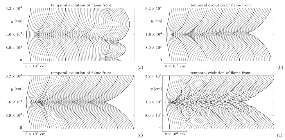
Figure 4: Evolution of the flame front at $\rho_{u}=5\times 10^{7}\mathrm{g}\,\mathrm{cm}^{-3}$. The contours mark evolution steps of 2.5 ms; (a) resolution 50$\times$50 cells; (b) resolution 100$\times$100 cells; (c) resolution 200$\times$200 cells; (d) resolution 400$\times$400 cells;

The planar flame was initially perturbed in a sinusoidal way with an amplitude of 640 cm. But note that the length scales are arbitrary since the problem is scale-invariant. In the plots each contour is shifted artificially into the $x$-direction for better visibility and corresponds to a time evolution of 2.5 ms. The $x$-coordinate is stretched by a factor of about 2. In all cases the initial perturbation grows and a cellular flame shape emerges. For comparison we also computed the propagation of a initially planar flame front in the same setup and with a resolution of $400\times 400$ cells over the same time period. We found no sign of any deviation of the flame shape from its initial planar configuration.

5.2 The Landau-Darrieus instability

Our first task was to measure the growth of the amplitude of the perturbation and to compare it to the theoretical prediction (eq. (2)). This was done by a simple determination of the distance between the rightmost and the leftmost points of the flame front. Figure 5 shows the growth rate of the perturbation amplitude over time. The dashed line corresponds to Landau’s dispersion relation. All results share the feature that the growth of the amplitude is shifted in the beginning. This comes from the fact that we impose an initial perturbation but not the corresponding flow field. Thus some set-up period is necessary for the correct velocities to build up in the vicinity of the flame front. In Figure 5, the linear regime of perturbation growth can be clearly distinguished from the later nonlinear stage, where the perturbation amplitude saturates. We will now discuss the linear part of the flame evolution.

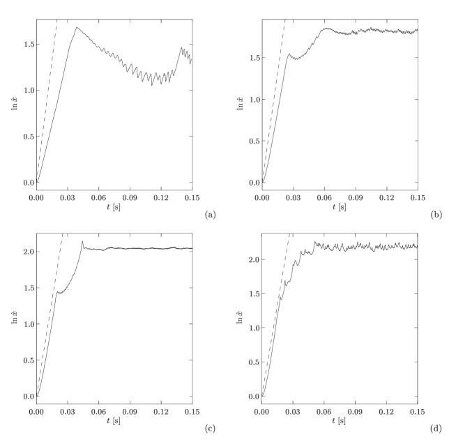
Figure 5: Perturbation amplitudes $\ln\hat{x}$ as a function of time $t$; (a) resolution 50$\times$50 cells; (b) resolution 100$\times$100 cells; (c) resolution 200$\times$200 cells; (d) resolution 400$\times$400 cells;

It is evident from Figure 5 that the difference between the growth of the perturbation amplitude in our simulation and in theory decreases with resolution. According to Table 1 the deviation is about 46% for the $50\times 50$ cells simulation and only about 10% for the $200\times 200$ cells simulation. In the higher resolved runs the initial perturbation quickly gets superimposed with perturbations of higher wavenumber so that the values of the growth rate can not safely be assigned to the largest wavelength of perturbation anymore. This is the reason why it exceeds the theoretical expectation slightly. One could conclude from the results that the simulated growth rate matches the theoretical expectations better with higher resolution and converge for a resolution between 200 and 300 cells per dimension for our given fuel density. Alternatively an explanation could be given in terms of a finite effective flame thickness. Even with the special measures described in § 4 $d_{l}$ can not be expected to be smaller than one cell width. A theoretical approximation of a finite flame width is the assignment of a curvature-dependent flame speed:

$$s=s_{l}(1-l_{\mathrm{M}}\kappa),$$ (18)

Here $\kappa$ denotes the curvature of the flame front and $l_{\mathrm{M}}$ is the phenomenological Markstein length that is related to the flame width. This burning law changes the dispersion relation in dependence of the Markstein length. In our case one would expect the Markstein length to be higher for less resolved simulations. The question whether the Markstein relation is appropriate to describe the behavior of our flame front is subject to a different study which will be presented elsewhere.

Table 1: Growth rate of perturbation amplitude

Case	$\omega$
Theory	88.7
$50\times 50$ cells	47.8
$100\times 100$ cells	69.0
$200\times 200$ cells	79.7
$300\times 300$ cells	90.0
$400\times 400$ cells	91.4

The sequence of plots in Figure 5 shows increasing similarity of the overall evolution of the amplitudes with higher resolution. This indicates that our numerical model of the LD instability in thermonuclear flames converges in the global properties.

5.3 Cellular stabilization

Figure 4 clearly shows the transition in flame propagation from the linear regime in the beginning, where perturbation growth by virtue of the LD instability dominates the dynamics, to the nonlinear burning regime. In accord with theoretical expectations (§ 3) this happens by the formation of cusps in recesses of the front. The flame adopts a cellular shape.

The global picture of the cellular regime is similar in all resolutions but the evolution of the shape differs in details. This difference is most prominent in the lowest resolved flame where the cell splits and a two-cell structure forms. As reported by Joulin (1994) the phenomenon of cell splitting is not supported by analytical investigations of the nonlinear regime, but this could be owing to the restricted class of solutions studied there. Its invocation is usually attributed to numerical noise. This would explain why this feature is observed in the low-resolution simulation where the discretization errors are large.

All other runs share the feature that the final outcome is a single-cell structure which steadily propagates forward. An effect contrary to the deviation in low resolved simulations is that with increasing resolution perturbations of smaller wavelength become observable that superimpose the initial long-wavelength perturbation. This is evident for the highest resolved run. The small cells superimposed to the large cell propagate downward to the cusp where they disappear. Again, the invocation of this phenomenon is discussed controversially in literature and Joulin (1994, 1989) argues that it should be attributed to numerical noise (as roundoff and truncation errors). It is even present in highly accurate numerical solutions of the Sivashinsky-equation. However, a prerequisite for its observation is a wide enough computational domain (in our case a sufficiently high resolution in $y$-direction), as reported by Gutman & Sivashinsky (1990). The reason why a superimposed smaller-wavelength cellular pattern does not destroy the global cusp-like structure although its amplitude should grow faster due to the higher wavenumber (see eq. (2)) was explained by Zel’dovich et al. (1980) on the basis of a WKB-like linear analysis and by Joulin (1989) in the nonlinear regime. The origin of the effect lies in a flow component parallel to the flame with increasing velocity towards the cusp. Therefore the superimposed perturbation is advected towards the cusp while its wavelength is stretched. In that way their grows is reduced until they disappear in the cusp. This is exactly what we observe in our highest-resolved simulation.

5.4 Increase in flame surface and acceleration of the flame

The wrinkling of the flame front amplified by the LD instability increases the flame surface. This causes the mean fuel consumption rate to grow and the flame is expected to propagate with an increased mean velocity $v_{\mathrm{mean}}$,

$$\frac{v_{\mathrm{mean}}(t)}{v_{\mathrm{mean}}(t_{0})}=\frac{A(t)}{A(t_{0})},$$ (19)

where $A(t)$ is the flame surface area (i.e. length of the one-dimensional flame in our two-dimensional simulation) at time $t$. In Figure 6 we present a measurement of the temporal evolution of the flame surface area and the mean velocity. As expected, the evolution of the velocities follows the growth of the initial perturbations in the beginning and saturates in the cellular regime. The flame area in Figure 6 is normalized to the flame area of our initial configuration whereas the mean velocity is normalized to the laminar flame speed. This results in a shift between $v_{\mathrm{mean}}(t)/s_{l}$ and ${A(t)/A(t_{0})}$ because the initial configuration is already perturbed from the planar shape and the corresponding value of the mean velocity deviates from $s_{l}$. The flow field needs some time to adapt to the initial flame geometry. Figure 6 (c) depicts the difference between $v_{\mathrm{mean}}(t)/s_{l}$ and ${A(t)/A(t_{0})}$. Apart from the initial shift there is a deviation which can partly be explained by the different methods of measurement. While the mean propagation velocity was calculated from the flame positions which were determined by the contents of ashes in the grid cells, the flame surface area was obtained by linear interpolation of the zero level-set of the $G$-function in the cells. Additionally one has to keep in mind that (19) holds strictly only for a burning velocity that is constant over the flame front. This is probably not fulfilled in our simulation since we would expect an intrinsic Markstein-like behavior as discussed above.

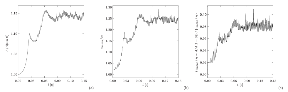
Figure 6: Growth of flame surface area (a) and mean velocity (b) for a resolution of 100$\times$100 cells; (c) deviation of area and velocity

5.5 Robustness of the numerical scheme

Reinecke et al. (1999) reported difficulties with the implementation of the complete version of the level set method. We examined our implementation in order to evaluate the improvements that could be achieved to stabilize the algorithm. Robustness of the reconstruction scheme is a prerequisite for its application to more complex simulations such as flame evolution in presence of imprinted turbulence or type Ia supernova explosions.

From given pre- and post-front states which exactly fulfill the Rankine-Hugoniot jump conditions Reinecke et al. (1999) synthesize a mixed cell according to (8)–(10) for a given volume fraction of unburnt material $\alpha_{0}$. While trying to reconstruct for the burnt and unburnt states imposing an unburnt volume fraction $\alpha$ that deviates slightly from the exact value $\alpha_{0}$, they find that the solver for the nonlinear reconstruction equation system can enter values for which the equation of state is undefined. It reaches values for the internal energy of the unburnt material which are lower than the internal energy belonging to zero temperature. This, of course means that the reconstruction fails. The problem is caused by the degenerate equation of state and is not observed in simulations of chemical deflagration fronts.

In simulations of thermonuclear flames this is a serious obstacle to build a stable implementation, because the flame front is linearly interpolated in mixed cells and therefore $\alpha$ deviates from the exact value. This deviation becomes most pronounced in highly curved front geometries. One would expect higher orders of interpolation to cure this problem. This, however, would strongly increase the number of topological uncertainties of the kind depicted in the rightmost sketch of Figure 2.

The described difficulty remains a critical issue in our simulations. It occurs when the front is highly curved. This is especially the case for cusps of cellular stabilized front geometries. Here situations are possible which lead to a large deviation of the $\alpha$-value determined by linear interpolation from the intersection points of cell borders with zero level set of $G$ and the actual $\alpha_{0}$ given by the exact shape of the zero level line of $G$, as illustrated in Figure 7.

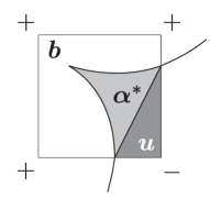
Figure 7: Critical situation: the region marked with $\alpha^{*}$ is the deviation between the actual $\alpha_{0}$ and $\alpha$ determined by linear interpolation

In these cases energy is added to the cell to obtain a physical unburnt state with positive temperature. This of course makes our numerical scheme slightly non-conservative. Fortunately, the cases where cusps are aligned in an unfavorable manner with respect to the computational grid are rare. Of course, as stated by Reinecke et al. (1999), a straight forward method to extenuate the problem is to limit the flame curvature by introducing a curvature-dependent effective burning velocity according to (18). The curvature $\kappa$ of the flame front can be easily determined from $G$. In the presented simulations we did not explicitly prescribe a burning law according to (18). For reasons discussed in § 5.2 a Markstein-like behavior may be present for numerical reasons, but a larger Markstein length might contribute to the robustness of the in-cell reconstruction scheme.

A further issue in the Reinecke et al. (1999) implementation is that the implicit treatment of the source terms in the reconstruction scheme (see § 4.1.2) was not applied. This leads to an additional deviation of energy and species distribution from the zero level set of the $G$-function. Implementation of this method in our code made the reconstruction scheme more reliable.

6 Conclusion

As stated in the introduction, a thorough understanding of the flame propagation in SN Ia on intermediate scales may be crucial to explain these astrophysical events. To summarize the contribution of the presented work to that issue it seems appropriate to repeat briefly the current status of research in the area of thermonuclear flame propagation in SN Ia in connection to the LD instability.

After the pioneering work of Timmes & Woosley (1992) which in detail described the one-dimensional structure of thermonuclear flames in white dwarf matter there have been several attempts to investigate the propagation of two-dimensional flames. Niemeyer & Hillebrandt (1995) were the first to confirm by means of a hydrodynamical simulation that thermonuclear flames in white dwarf matter are indeed subject to the LD instability. They were, however, not able to reach the nonlinear regime of flame propagation, where the flame is expected to stabilize in a cellular shape. This phenomenon was subject to other investigations, e.g. Bychkov & Liberman (1995) and Blinnikov & Sasorov (1996). These studies are, however, based on the investigation of the Sivashinsky equation and do not solve the full hydrodynamical problem. Thus, although the assumption that the flame is nonlinearly stabilized is supported by these investigations, it can not be considered as proven.

With the presented numerical model we were able to confirm the statement of Niemeyer & Hillebrandt (1995) that nuclear burning fronts in white dwarfs are subject to the LD instability on scales larger than the flame width. The growth rate of perturbation amplitude in the linear regime of the flame propagation is in reasonable agreement with the theoretical prediction for sufficient spatial resolution. Beyond the results of Niemeyer & Hillebrandt (1995) we observe the transition from linear to nonlinear propagation regime. The formation of cusps pointing towards the burnt material stabilizes the flame in a cellular shape. This has been observed and theoretically interpreted for terrestrial flames and is now demonstrated by means of a full hydrodynamical simulation for astrophysical flames for the first time. With the increase of the flame surface we note a flame acceleration which saturates at about 1.3 times the laminar flame velocity when the flame has settled in its steady cellular structure.

All our simulations with sufficient resolution finally yield a flame in the shape of a single domain-filling cell and with higher resolution this basic shape gets superimposed with small cells. This in in excellent agreement with results from numerical simulations of the Sivashinsky-equation. Gutman & Sivashinsky (1990) study the flame evolution according to this equation numerically using a simulation set-up similar to ours. While their method is a semianalytical approach they find effects which are very similar to our results. For domains only a few times larger than the critical wavelength corresponding to the maximum amplification rate they find a time-independent cusp-like structure emerging. For larger domains (some ten times the critical wavelength) they observe a time-dependent pattern of small-scale cells superimposed to the cusp. They argue that this is caused by an increased sensitivity of large-scale configurations at wide intervals to small perturbations. Therefore the observed small-scale cells are attributed to weak numerical noise rather than being a self-sustaining phenomenon. We believe that this is the case in our simulations, too. The observation of a similar behavior in our model rules out the possibility that the effect is a peculiarity of the numerical solution of the Sivashinsky equation. Further discussion of the phenomenon and attempt for analytical treatment using the pole decomposition method for solving a modified Sivashinsky-equation can be found in Joulin (1989) and Joulin (1994).

Whether other geometries (like the spherically expanding flame investigated by Blinnikov & Sasorov (1996)) would lead to a repeated cell-splitting needs further investigation.

Niemeyer & Hillebrandt (1995) report a break-up of the cellular stabilization at a fuel density of $5\times 10^{7}\mathrm{g}\,\mathrm{cm}^{-3}$. Our simulations were performed at the same density of the unburnt material and do not show this feature. This is, however, not necessarily a contradiction since it is possible that perturbations as a result of numerical noise, which is different in the two implementations, could trigger the break-up. This scenario is not unrealistic since one would expect physical noise to be present in SN Ia explosions. The possibility of a loss of nonlinear stabilization and self-turbulization of the flame front leading to active turbulent combustion remains an open question that is of great importance for large scale supernova simulations. This topic will be investigated in a subsequent study aiming at the simulation of the interaction of the LD instability with imprinted turbulence. Here the flame is exposed to a “controlled noise”, which can be quantified. From the results of numerical simulations it is evident that our model of thermonuclear flames is an adequate tool for this task.

References

- Audi & Wapstra (1995) Audi, G. & Wapstra, A. H. 1995, Nucl. Phys. A, 595, 409
- Blinnikov & Sasorov (1996) Blinnikov, S. I. & Sasorov, P. V. 1996, Phys. Rev. E, 53, 4827
- Bychkov & Liberman (1995) Bychkov, V. & Liberman, M. A. 1995, A&A, 302, 727
- Colella & Woodward (1984) Colella, P. & Woodward, P. R. 1984, J. Comp. Phys., 54, 174
- Cox & Giuli (1968) Cox, J. P. & Giuli, R. T. 1968, Principles of Stellar Structure, Vol. 2 (New York: Gordon and Breach)
- Darrieus (1938) Darrieus, G. 1938, communication presented at La Technique Moderne, Unpublished.
- Frankel (1990) Frankel, M. L. 1990, Phys. Fluids, A, 2, 1879
- Fryxell et al. (1989) Fryxell, B. A., Müller, E., & Arnett, W. D. 1989, MPA Preprint, 449
- Gutman & Sivashinsky (1990) Gutman, S. & Sivashinsky, G. I. 1990, Physica D, 43, 129
- Helenbrook & Law (1999) Helenbrook, B. T. & Law, C. K. 1999, Combustion and Flame, 117, 155
- Hillebrandt & Niemeyer (2000) Hillebrandt, W. & Niemeyer, J. C. 2000, ARA&A, 38, 191
- Höflich & Khokhlov (1996) Höflich, P. & Khokhlov, A. 1996, ApJ, 457, 500
- Ivanova et al. (1974) Ivanova, L. N., Imshennik, V. S., & Chechetkin, V. M. 1974, Ap&SS, 31, 497
- Iwamoto et al. (1999) Iwamoto, K., Brachwitz, F., Nomoto, K., Kishimoto, N., Umeda, H., Hix, W. R., & Thielemann, F. 1999, ApJS, 125, 439
- Joulin (1989) Joulin, G. 1989, J. Phys. France, 50, 1069
- Joulin (1994) Joulin, G. 1994, Phys. Rev. E, 50, 2030
- Kerstein (1996) Kerstein, A. R. 1996, Combust. Sci. Technol., 118, 189
- Khokhlov (1991) Khokhlov, A. M. 1991, A&A, 245, 114
- Landau (1944) Landau, L. D. 1944, Acta Physicochim. URSS, 19, 77
- Moré et al. (1980) Moré, J. J., Garbow, B. S., & Hillstrom, K. E. 1980, User Guide for MINPACK-1, Argonne National Laboratory Report ANL-80-74 (Argonne, Ill.: Argonne National Laboratory)
- Niemeyer (1998) Niemeyer, J. C. 1998, in Stellar Evolution, Stellar Explosions and Galactic Chemical Evolution, ed. A. Mezzacappa (Bristol and Philadelphia: Institute of Physics Publishing), 673–680
- Niemeyer (1999) Niemeyer, J. C. 1999, ApJ, 523, L57