Nonadiabatic resonant dynamic tides and orbital evolution in close binaries

This investigation is devoted to the effects of nonadiabatic resonant dynamic tides generated in a uniformly rotating stellar component of a close binary. The companion is considered to move in a fixed Keplerian orbit, and the effects of the centrifugal force and the Coriolis force are neglected. Semi-analytical solutions for the linear, nonadiabatic resonant dynamic tides are derived by means of a two-time variable expansion procedure. The solution at the lowest order of approximation consists of the resonantly excited oscillation mode and displays a phase shift with respect to the tide-generating potential. Expressions are established for the secular variations of the semi-major axis, the orbital eccentricity, and the star’s angular velocity of rotation caused by the phase shift. The orders of magnitude of these secular variations are considerably larger than those derived earlier by Zahn (1977) for the limiting case of dynamic tides with small frequencies. For a $5\,M_{\odot}$ ZAMS star, an orbital eccentricity $e=0.5$, and orbital periods in the range from 2 to 5 days, numerous resonances of dynamic tides with second-degree lower-order $g^{+}$-modes are seen to induce secular variations of the semi-major axis, the orbital eccentricity, and the star’s angular velocity of rotation with time scales shorter than the star’s nuclear life time.

1 Introduction

Various investigations have already been devoted to tidal actions in components of close binaries and their effects on orbital evolution.

A commonly used approach for the study of dynamic tides rests on a Fourier decomposition of the tide-generating potential in terms of multiples of the orbital frequency. For each forcing frequency, the dynamic tide is then determined by integration of the system of differential equations governing linear, forced oscillations of an equilibrium star on the assumption of a fixed orbit.

Zahn (1975) used this approach in order to determine the influence of the radiative damping in the nonadiabatic surface layers of a spherically symmetric star on low-frequency dynamic tides. He considered a star consisting of a convective core and a radiative envelope. In developing an asymptotic theory, he distinguished between the interior layers, where the forced oscillations are nearly isentropic, and a boundary layer, where the radiative damping is important.

Because of the radiative dissipation near the star’s surface, dynamic tides do not have the same properties of symmetry as the exciting potential, so that the companion exerts a torque on the star which may tend to synchronise the star’s rotation with the orbital motion. According to Zahn, the torque appears to be strong enough to achieve synchronisation, for relatively close binaries, in a time short in comparison with the star’s nuclear life time. Consequently, Zahn considered dynamic tides with radiative dissipation as an efficient process for the synchronisation of components of close binaries that do not have a convective envelope.

A generalisation of Zahn’s treatment to include the effects of the Coriolis force in the case of a slowly rotating component was given by Rocca (1989).

The system of equations governing the non-adiabatic tidal response of a spherically symmetric star was integrated numerically by Savonije & Papaloizou (1983). For simplicity, the authors restricted themselves to small orbital eccentricities and neglected the perturbation of the gravitational potential caused by the tidal response. They presented results for main sequence, non-rotating tidally distorted stars and concluded that the “the spin up of the massive component appears to be rather inefficient …, unless the system could be locked into resonance …”. Subsequently, Savonije & Papaloizou (1984) determined the tidal response for an evolved stellar model of $20\,M_{\odot}$ and found a substantial increase of the effectiveness of tidal evolution during the late phases of core hydrogen burning.

On his side, Tassoul (1987) argued that the general trend toward synchronism that is found in early-type binaries, cannot be explained solely by Zahn’s theory on the action of radiative damping on dynamic tides. He presented a hydrodynamical mechanism involving large-scale, mechanically driven currents which transport angular momentum.

More recently, the work of Savonije & Papaloizou was extended by a series of investigations on uniformly rotating spherically symmetric stars in which the effects of the Coriolis force were taken into account (Savonije et al., 1995; Papaloizou & Savonije, 1997; Savonije & Papaloizou, 1997; Lai, 1997; Witte & Savonije, 1999a).

The effect of resonance locking on the tidal evolution of massive binaries was studied by Witte & Savonije (1999b, 2001). The authors concluded that when both orbital and stellar evolution are taken into account, a dynamic tide can easily become locked in a resonance for a prolonged period of time. They furthermore found that, during a resonance, a significant enhancement of the secular evolution of the semi-major axis and the orbital eccentricity occurs.

In this study, our aim is first to describe the influence of the perturbation of the radiative energy transfer on tidal resonances with free oscillation modes in components of close binaries. To this end, we use a two-time variable expansion procedure leading to semi-analytical solutions for the resonant dynamic tides and the resulting perturbation of the star’s external gravitational field. This investigation is an extension of an earlier investigation of Smeyers et al. (1998) (hereafter referred to as Paper I), in which the resonant dynamic tides were treated in the isentropic approximation.

In the second part of our investigation, we determine the effects of the nonadiabaticity of the tidal motions on the orbital evolution of a close binary in cases of resonances of dynamic tides with free oscillation modes $g^{+}$.

We consider a uniformly rotating component of a close binary but we still neglect the effects of the centrifugal force and the Coriolis force on the resonant dynamic tides.

The plan of the paper is as follows. In Sect. 2, we present the basic assumptions and the equations governing nonadiabatic forced oscillations of a rotating spherically symmetric star. In Sect. 3, the tide-generating potential is expanded in terms of spherical harmonics and in Fourier series in terms of the companion’s mean motion. In Sect. 4, we derive the lowest-order solutions for the nonadiabatic resonant dynamic tides. Sect. 5 is devoted to the derivation of the equations governing the secular changes of the semi-major axis, the orbital eccentricity, and the longitude of the periastron due to the perturbation of the star’s external gravitational field. In Sect. 6, we determine the torque exerted by the companion on the tidally distorted star and the associated rate of secular change of the star’s rotational angular velocity. In Sect. 7, we present phase shifts for resonant dynamic tides in a $5\,M_{\odot}$ zero-age main sequence star. We also consider time scales of orbital evolution for short orbital periods ranging from 2 to 5 days and for the orbital eccentricity $e=0.5$. Finally, Sect. 8 is devoted to concluding remarks.

2 Basic assumptions and governing equations

Consider a close binary system of stars with masses $M_{1}$ and $M_{2}$ that are orbiting around each other under the influence of their mutual gravitational force. The first star is assumed to rotate uniformly around an axis perpendicular to the orbital plane in the sense of the orbital motion, and the second star, called the companion, is considered to be a point mass describing a fixed Keplerian orbit around the star.

As in Paper I, we describe the oscillations of the star with respect to a corotating frame of reference $C_{1}x^{\prime\prime 1}x^{\prime\prime 2}x^{\prime\prime 3}$ whose origin coincides with the mass centre $C_{1}$ of the star and whose $x^{\prime\prime 1}x^{\prime\prime 2}$-plane coincides with the orbital plane of the binary. The direction of the $x^{\prime\prime 3}$-axis corresponds to the direction of the star’s angular velocity $\@vec{\Omega}$. With respect to this corotating frame of reference, we introduce a system of spherical coordinates $\@vec{r}=(r,\theta,\phi)$. We consider the spherical coordinates $r$, $\theta$, $\phi$ as generalised coordinates $q^{1}$, $q^{2}$, $q^{3}$.

The tidal force generated by the companion is introduced as a small time-dependent force which perturbs the hydrostatic equilibrium of a spherically symmetric static star. Correspondingly, the tide generated by the companion is considered as a forced perturbation of the star’s equilibrium.

Let $\varepsilon_{T}W\left(\@vec{r},t\right)$ be the tide-generating potential, where $\varepsilon_{T}$ is a small dimensionless parameter defined as

$$\varepsilon_{T}=\left({R_{1}\over a}\right)^{3}\,{M_{2}\over M_{1}}.$$ (1)

Here $R_{1}$ is the radius of the spherically symmetric equilibrium star, and $a$ the semi-major axis of the companion’s relative orbit.

Furthermore, let $\left(\delta q^{j}\right)_{T}$, with $j=1,2,3,$ be the contravariant components of the tidal displacement in the star with respect to the local coordinate basis $\partial/\partial q^{1}$, $\partial/\partial q^{2}$, $\partial/\partial q^{3}$. If one neglects the effects of the centrifugal force and the Coriolis force, these components are governed by the equations

$$g_{ij}\,{{\partial^{2}\left(\delta q^{j}\right)_{T}}\over{\partial t^{2}}}+U_{ij}\left(\delta q^{j}\right)_{T}=-\varepsilon_{T}\,{{\partial W}\over{\partial q^{i}}},\,\,\,i=1,2,3.$$ (2)

The $g_{ij}$ are the components of the metric tensor, and the $U_{ij}$ the tensorial operators applying to free linear, isentropic oscillations of a spherically symmetric star, which are defined by

$$U_{ij}\left({\delta q^{j}}\right)_{T}={{\partial\left(\delta\Phi\right)_{T}}\over{\partial q^{i}}}-{{\left(\delta\rho\right)_{T}}\over{\rho^{2}}}\,{{\partial P}\over{\partial q^{i}}}+{1\over\rho}\,{{\partial\left(\delta P\right)_{T}}\over{\partial q^{i}}}.$$ (3)

In these equations, $P$ is the pressure, $\rho$ the mass density, and $\Phi$ the gravitational potential. When the operator $\delta$ is applied to a quantity, the Lagrangian perturbation of that quantity is taken.

The Lagrangian perturbations of the mass density and the gravitational potential are determined by the equation expressing the conservation of mass

$${{\left(\delta\rho\right)_{T}}\over\rho}=-\nabla_{j}\left(\delta q^{j}\right)_{T}$$ (4)

and by Poisson’s integral equation

$$\left(\delta\Phi\right)_{T}=\left(\delta q^{j}\right)_{T}\nabla_{j}\Phi$$ (5)

$$-G\int_{V}\rho\left(\@vec{r^{\prime}}\right)\left(\delta q^{\prime j}\right)_{T}\left(\@vec{r^{\prime}}\right)\left[\nabla_{\prime j}|\@vec{r}-\@vec{r^{\prime}}|^{-1}\right]dV\left(\@vec{r^{\prime}}\right).$$

In the latter equation, $G$ is the gravitational constant, and $V$ the volume of the spherically symmetric equilibrium star. The operators $\nabla_{j}$ and $\nabla_{\prime j}$ are the operators of partial differentiation with respect to the generalised coordinates $q^{j}$ and $q^{\prime j}$ when they are applied to a scalar quantity, and are the operators of covariant differentiation when they are applied to a vector or a tensor component.

For tides considered as linear, nonadiabatic forced perturbations of the spherically symmetric equilibrium star, the Lagrangian perturbation of the pressure is determined by the equation for the rate of change of thermal energy

$${\partial\over{\partial t}}\left[{{\left(\delta P\right)_{T}}\over P}-\Gamma_{1}{{\left(\delta\rho\right)_{T}}\over\rho}\right]={{\left(\Gamma_{3}-1\right)\rho}\over P}\,\left(\delta\,{{dQ}\over{dt}}\right)_{T}.$$ (6)

Here $\Gamma_{1}\equiv(\partial\ln P/\partial\ln\rho)_{S}$ and $\Gamma_{3}-1\equiv(\partial\ln T/\partial\ln\rho)_{S}$ are generalised isentropic coefficients, $T$ is the temperature, and $dQ/dt$ is the rate of energy exchange per unit time and unit mass. In the regions of the star where the energy transfer is purely radiative, $dQ/dt$ is given by

$${{dQ}\over{dt}}=\varepsilon_{1}-{1\over\rho}\,\nabla\cdot\@vec{F}_{\rm R},$$ (7)

where $\varepsilon_{1}$ is the amount of energy generated by the thermonuclear reactions per unit time and unit mass, and $\@vec{F}_{\rm R}$ the radiative energy flux.

We make the equations dimensionless by expressing the time $t$, the radial coordinate $r$, the mass density $\rho$, the pressure $P$, both the gravitational potential $\Phi$ and the tide-generating potential $\varepsilon_{T}\,W$, and the rate of energy exchange per unit mass $dQ/dt$ respectively in the units $\left[R_{1}^{3}/(GM_{1})\right]^{1/2}$, $R_{1}$, $M_{1}/\left(4\pi R_{1}^{3}\right)$, $GM_{1}^{2}/\left(4\pi R_{1}^{4}\right)$, $GM_{1}/R_{1}$, and $L_{1}/M_{1}$, where $L_{1}$ is the luminosity of the star.

Furthermore, we express the Lagrangian perturbation of the rate of energy exchange during the tidal motions formally in terms of the components of the tidal displacement as

$$\left(\delta\,{{dQ}\over{dt}}\right)_{T}={\cal V}_{j}\left(\delta q^{j}\right)_{T},$$ (8)

where the ${\cal V}_{j}$ are linear operators. Eq. (6) for the rate of change of thermal energy can then be rewritten as

$${\partial\over{\partial t}}\!\left[{{\left(\delta P\right)_{T}}\over P}+\Gamma_{1}\nabla_{j}\!\left(\delta q^{j}\right)_{T}\right]\!=C\,{{\left(\Gamma_{3}-1\right)\rho}\over P}\,{\cal V}_{j}\left(\delta q^{j}\right)_{T},$$ (9)

where

$$C\equiv\left({R_{1}^{3}\over{G\,M_{1}}}\right)^{1/2}/\left({{G\,M_{1}^{2}}\over{R_{1}\,L_{1}}}\right)$$ (10)

is the ratio of the dynamic time scale to the Helmholtz-Kelvin time scale of the star.

3 The tide-generating potential

Following Polfliet & Smeyers (1990), we expand the tide-generating potential in terms of unnormalised spherical harmonics $Y_{\ell}^{m}(\theta,\phi)$ and in Fourier series in terms of multiples of the companion’s mean motion $n$. The expansion takes the form

$$\varepsilon_{T}\,W\left(\@vec{r},t\right)=\varepsilon_{T}\,\sum_{\ell=2}^{4}\sum_{m=-\ell}^{\ell}\sum_{k=-\infty}^{\infty}W_{\ell,m,k}\left(\@vec{r}\,\right)$$ (11)

$$\exp\left[{\rm i}\left(\sigma_{T}\,t-k\,n\,\tau\right)\right],\hskip 85.35826pt$$

where

$$W_{\ell,m,k}\left(\@vec{r}\,\right)=-c_{\ell,m,k}\,\left({r\over R_{1}}\right)^{\ell}\,Y_{\ell}^{m}(\theta,\phi),$$ (12)

$\sigma_{T}$ is the forcing angular frequency with respect to the corotating frame of reference determined as

$$\sigma_{T}=k\,n+m\,\Omega,$$ (13)

and $\tau$ is a time of periastron passage. The Fourier coefficients $c_{\ell,m,k}$ are defined as

$$c_{\ell,m,k}=\displaystyle{{(\ell-|m|)!}\over{(\ell+|m|)!}}\,P_{\ell}^{|m|}(0)\left({R_{1}\over a}\right)^{\ell-2}{1\over{\left({1-e^{2}}\right)^{\ell-1/2}}}$$ (14)

$${1\over\pi}{\int_{0}^{\pi}(1+e\,\cos v)^{\ell-1}\,\cos(k\,M+m\,v)\,dv}.$$

In this definition, $P_{\ell}^{|m|}(x)$ is an associated Legendre polynomial of the first kind, and $M$ and $v$ are respectively the mean and the true anomaly of the companion in its relative orbit.

¿From Definition (14), it follows that the Fourier coefficients $c_{\ell,m,k}$ depend on the orbital eccentricity. They decrease as the multiple $k$ of the mean motion increases. The decrease is slower for higher orbital eccentricities. Consequently, the number of terms that has to be taken into account in Expansion (11) of the tide-generating potential increases with increasing values of the orbital eccentricity. For illustration, the logarithms of the absolute values of the second-degree Fourier coefficients $c_{2,m,k}$, with $m=-2,0,2$, are displayed in Fig. 1 as functions of $k$ for the orbital eccentricities $e=0.25$ and $e=0.5$.

Figure 1: Logarithmic representation of the absolute values of the Fourier coefficients $c_{2,m,k}$, with $m=-2,0,2$, as functions of $k$, for the orbital eccentricities $e=0.25$ (solid circles) and $e=0.5$ (open circles).

4 Lowest-order solutions for nonadiabatic resonant dynamic tides

We consider a single partial dynamic tide generated by the term

$$\varepsilon_{T}\,W_{\ell,m,k}\left(\@vec{r}\,\right)\,\exp\left[{\rm i}\left(\sigma_{T}\,t-k\,n\,\tau\right)\right]$$ (15)

of Expansion (11) of the tide-generating potential, and assume that its forcing angular frequency $\sigma_{T}$ is close to the degenerate eigenfrequency $\sigma_{\ell,N}$ of the star’s free linear, isentropic oscillation modes of radial order $N$ that belong to the spherical harmonics $Y_{\ell}^{m}(\theta,\phi)$ of degree $\ell$ and the various admissible azimuthal numbers $m$. We define the relative frequency difference $\varepsilon$ as

$$\varepsilon={{\sigma_{\ell,N}-\sigma_{T}}\over{\sigma_{\ell,N}}}$$ (16)

and assume $\varepsilon$ to be of the order of $\varepsilon_{T}$:

$$\varepsilon=f\,\varepsilon_{T},\,\,\,f\in{\rm I\!R}.$$ (17)

In addition, we consider the nonadiabatic effects, which are rendered by the right-hand member of Eq. (9), to be of the order of $\varepsilon_{T}$ at least in some region near the star’s surface and, for convenience, set

$$C=C^{\prime}\,\varepsilon_{T},\,\,\,C^{\prime}\,\in{\rm I\!R}.$$ (18)

We determine the combined effects of the resonance of the dynamic tide and the nonadiabaticity of the tidal motions by means of an appropriate two-time variable expansion procedure (Kevorkian & Cole 1981, Section 3.2.7; 1996, Section 4.3.1). In this expansion procedure, the nonadiabatic terms are evaluated in the quasi-isentropic approximation. A similar perturbation procedure was used by Terquem et al. (1998) for the evaluation of the nonadiabaticity of tidal motions.

In view of the application of the two-time variable expansion procedure, we pass on to a new dimensionless time variable

$$t^{\ast}=\sigma_{\ell,N}\,t.$$ (19)

Adopting $\varepsilon_{T}$ as the small expansion parameter, we introduce a fast and a slow time variable as

$$t^{+}=t^{\ast}\left[1+O\left(\varepsilon_{T}^{2}\right)\right]$$ (20)

and

$$\tilde{t}=\varepsilon_{T}\,t^{\ast},$$ (21)

and expand the components of the tidal displacement in terms of the star’s linear, isentropic oscillation modes $s^{\prime}$ as

$$\left(\delta q^{j}\right)_{T}\left(\@vec{r},t\right)=\sum_{s^{\prime}}\Bigl{[}\sum_{n=0}^{\infty}\varepsilon_{T}^{n}F_{s^{\prime}}^{(n)}\left(t^{+}\!,\tilde{t}\,\right)\Bigr{]}\left(\delta q^{j}\right)_{s^{\prime}}\!\left(\@vec{r}\right),$$ (22)

where $j=1,2,3$. The expansions can be restricted to the star’s spheroidal modes, since neither the tidal force nor the nonadiabatic effects produce any vorticity around the normal to the local spherical equipotential surface of the equilibrium star. A given spheroidal mode $s^{\prime}$ is characterised by the degree $\lambda^{\prime}$ and the azimuthal number $\mu^{\prime}$ of the spherical harmonic to which it belongs, and by the radial order $\nu^{\prime}$. The components of the Lagrangian displacement and the angular eigenfrequency of the oscillation mode $s^{\prime}$ obey the wave equations

$$\sigma^{2}_{\lambda^{\prime}\!,\nu^{\prime}}\,g_{ij}\left({\delta q^{j}}\right)_{\lambda^{\prime}\!,\mu^{\prime}\!,\nu^{\prime}}\!-U_{ij}\left({\delta q^{j}}\right)_{\lambda^{\prime}\!,\mu^{\prime}\!,\nu^{\prime}}\!=0,\,\,\,i=1,2,3.$$ (23)

We also introduce an expansion for the Lagrangian perturbation of the pressure as

$$\left(\delta P\right)_{T}\left(\@vec{r},t\right)=\sum_{n=0}^{\infty}\varepsilon_{T}^{n}\left(\delta P\right)_{T}^{(n)}\left(\@vec{r},t^{+}\!,\tilde{t}\,\right).$$ (24)

Substitution of Expansions (22) and (24) into Eq. (9), application of the chain rule, and integration with respect to the fast time variable yield, at order $\varepsilon_{T}^{0}$,

$${{\left(\delta P\right)_{T}^{(0)}}\over P}=-\Gamma_{1}\,\sum_{s^{\prime}}F_{s^{\prime}}^{(0)}\left(t^{+}\!,\tilde{t}\,\right)\nabla_{j}\left(\delta q^{j}\right)_{s^{\prime}}.$$ (25)

Introduction of the latter expansion into Eqs. (2) leads to the equations

$$g_{ij}\,{\partial^{2}\over{\partial t^{+2}}}\sum_{s^{\prime}}F_{s^{\prime}}^{(0)}\left(t^{+}\!,\tilde{t}\,\right)\!\left(\delta q^{j}\right)_{s^{\prime}}$$ (26)

$$+{1\over{\sigma^{2}_{\ell,N}}}\sum_{s^{\prime}}F_{s^{\prime}}^{(0)}\left(t^{+}\!,\tilde{t}\,\right)U_{ij}\!\left(\delta q^{j}\right)_{s^{\prime}}=0,\,\,\,i=1,2,3.$$

We transform these equations by using wave Eqs. (23) and multiplying all terms by $\rho\,\overline{\left({\delta q^{i}}\right)_{s}}$, where the bar denotes the complex conjugate, and $s$ stands for the degree $\lambda$, the azimuthal number $\mu$, and the radial order $\nu$ of a given spheroidal mode. Next, we integrate over the volume of the spherically symmetric equilibrium star and take into account the orthogonality property of the spheroidal modes. The resulting equation for the functions $F_{s}^{(0)}\left(t^{+}\!,\tilde{t}\,\right)$ takes the form

$${\partial^{2}\over{\partial t^{+2}}}\,F_{s}^{(0)}\left(t^{+}\!,\tilde{t}\,\right)+{\sigma^{2}_{\lambda,\nu}\over\sigma^{2}_{\ell,N}}\,F_{s}^{(0)}\left(t^{+}\!,\tilde{t}\,\right)=0.$$ (27)

A general solution is given by

$$F^{(0)}_{s}\left(t^{+}\!,\tilde{t}\,\right)=A^{(0)}_{s}\left(\tilde{t}\,\right)\exp\left(\mbox{i}{\sigma_{\lambda,\nu}\over\sigma_{\ell,N}}\,t^{+}\right),$$ (28)

where $A^{(0)}_{s}\left(\tilde{t}\,\right)$ is a yet undetermined complex function of the slow time variable $\tilde{t}$.

At order $\varepsilon_{T}$, substitution of Solutions (28) into Eq. (9) and integration with respect to the fast time variable yield

$${{\left(\delta P\right)_{T}^{(1)}}\over P}=-\Gamma_{1}\sum_{s^{\prime}}\bigg{\{}F_{s^{\prime}}^{(1)}\!\left(t^{+}\!,\tilde{t}\,\right)\nabla_{j}\!-{\rm i}\,C^{\prime}\,{{\left(\Gamma_{3}-1\right)\rho}\over P}$$ (29)

$$A^{(0)}_{s^{\prime}}\left(\tilde{t}\,\right)\sigma_{\lambda^{\prime},\nu^{\prime}}^{-1}\left[\exp\left({\rm i}\,{\sigma_{\lambda^{\prime},\nu^{\prime}}\over\sigma_{\ell,N}}\,t^{+}\right)\right]{\cal V}_{j}\bigg{\}}\left(\delta q^{j}\right)_{s^{\prime}}.$$

In this equality, the second term in the right-hand member is the contribution of the nonadiabatic effects to the Lagrangian perturbation of the pressure.

By proceeding in a similar way as for the derivation of Eq. (27), it follows that the functions $F_{s}^{(1)}\left(t^{+}\!,\tilde{t}\,\right)$ are governed by the inhomogeneous equation

$${\partial^{2}\over{\partial t^{+2}}}\,F_{s}^{(1)}\left(t^{+}\!,\tilde{t}\,\right)+{\sigma^{2}_{\lambda,\nu}\over\sigma^{2}_{\ell,N}}\,F_{s}^{(1)}\left(t^{+}\!,\tilde{t}\,\right)$$ (30)

$$=-2\,{\rm i}\,{{dA^{(0)}_{s}}\over{d\tilde{t}}}\,{\sigma_{\lambda,\nu}\over\sigma_{\ell,N}}\,\exp\left({\rm i}\,{\sigma_{\lambda,\nu}\over\sigma_{\ell,N}}\,t^{+}\right)$$

$$-\,{1\over{\sigma_{\ell,N}^{2}\,{\cal N}_{s}}}\,\left[\int_{V}\rho\,{{\partial W_{\ell,m,k}}\over{\partial q^{i}}}\,\overline{\left({\delta q^{i}}\right)_{s}}\,dV\right]$$

$$\;\;\;\Big{\{}\exp\left[-{\rm i}\left(f\,\tilde{t}+k\,n\,\tau\right)\,\right]\Big{\}}\exp\left({\rm i}t^{+}\right)$$

$$+\,{{{\rm i}\,C^{\prime}}\over{\sigma_{\ell,N}^{2}\,{\cal N}_{s}}}\!\sum_{s^{\prime}}\bigg{\{}\!\int_{V}\overline{\left(\delta q^{i}\right)_{s}}\,{{\partial\left[\left(\Gamma_{3}-1\right)\rho\,{\cal V}_{j}\left(\delta q^{j}\right)_{s^{\prime}}\right]}\over{\partial q^{i}}}\,dV\!\bigg{\}}$$

$$\sigma_{\lambda^{\prime},\nu^{\prime}}^{-1}\,A^{(0)}_{s^{\prime}}\left(\tilde{t}\,\right)\exp\left({\rm i}\,{\sigma_{\lambda^{\prime},\nu^{\prime}}\over\sigma_{\ell,N}}t^{+}\right),$$

where ${\cal N}_{s}$ is the square of the norm of the Lagrangian displacement for the oscillation mode $s$ [Paper I, Eq. (48)].

The integral contained in the second term of the right-hand member of Eq. (30) is developed in Eq. (44) of Paper I. After passing on to dimensionless quantities, one has

$$\int_{V}\rho\,{{\partial W_{\ell,m,k}}\over{\partial q^{i}}}\,\overline{\left({\delta q^{i}}\right)_{s}}\,dV=-\delta_{\lambda,\ell}\,\delta_{\mu,m}\,{{4\,\pi}\over{2\,\ell+1}}\,{{(\ell+|m|)!}\over{(\ell-|m|)!}}$$ (31)

$$c_{\ell,m,k}\int_{0}^{1}\ell\,r^{\ell-1}\left[{\xi_{\lambda,\nu}+(\ell+1)\,\eta_{\lambda,\nu}/r}\right]\rho\,r^{2}\,dr,$$

where $\delta_{\lambda,\ell}$ is a Kronecker’s delta, and $\xi_{\lambda,\nu}(r)$ and $\eta_{\lambda,\nu}(r)$ are the radial parts of the radial and the transverse component of the Lagrangian displacement [Paper I, Eqs. (43)].

The integral contained in the third term of the right-hand member of Eq. (30) can be transformed by means of Gauss’ theorem. If the mass density vanishes at the star’s surface, one derives that

$$\int_{V}\overline{\left(\delta q^{i}\right)_{s}}\,\left\{{\partial\over{\partial q^{i}}}\left[\left(\Gamma_{3}-1\right)\rho\,{\cal V}_{j}\left(\delta q^{j}\right)_{s^{\prime}}\right]\right\}dV$$ (32)

$$={{4\,\pi}\over{2\,\lambda+1}}\,{{(\lambda+|\mu|)!}\over{(\lambda-|\mu|)!}}\,\delta_{\lambda,\lambda^{\prime}}\,\delta_{\mu,\mu^{\prime}}$$

$$\int_{0}^{1}\left(\Gamma_{3}-1\right)\overline{\left(\delta\rho/\rho\right)_{\lambda,\nu}}\,\left[\delta\left(dQ/dt\right)\right]_{\lambda^{\prime},\nu^{\prime}}\rho\,r^{2}\,dr.$$

In the inhomogeneous part of Eq. (30), the resonant terms must be removed. We distinguish between two cases depending on whether the star’s spheroidal mode $s$ is equal to or different from the spheroidal mode with eigenfrequency $\sigma_{\ell,N}$ that belongs to the spherical harmonic $Y_{\ell}^{m}(\theta,\phi)$ and is involved in the resonance. We denote the latter spheroidal mode as the spheroidal mode $S$.

When $s=S$, the resonant terms are removed from the inhomogeneous part of Eq. (30) by setting

$$\displaystyle{{dA^{(0)}_{S}}\over{d\tilde{t}}}+C^{\prime}\,{\kappa_{\ell,N}\over\sigma_{\ell,N}}\,A^{(0)}_{S}$$ (33)

$$=\displaystyle{c_{\ell,m,k}\,Q_{\ell,N}\over{2\,{\rm i}}}\,\exp\left[-{\rm i}\left(f\,\tilde{t}+k\,n\,\tau\right)\right].$$

In this equation, the factor $Q_{\ell,N}$ is defined as

$$Q_{\ell,N}={1\over\sigma_{\ell,N}^{2}}{{\int_{0}^{R_{1}}\ell\,r^{\ell-1}\left[\xi_{\ell,N}+(\ell+1)\,\eta_{\ell,N}/r\right]\rho\,r^{2}\,dr}\over{\int_{0}^{R_{1}}\left[\xi^{2}_{\ell,N}+\ell(\ell+1)\,\eta^{2}_{\ell,N}/r^{2}\right]\rho\,r^{2}\,dr}}$$ (34)

[see Paper I, Eq. (50)], and $\kappa_{\ell,N}$ is the star’s coefficient of vibrational stability for the spheroidal mode $S$ defined as

$$\kappa_{\ell,N}=-{{\int_{0}^{1}\left(\Gamma_{3}-1\right)\overline{\left(\delta\rho/\rho\right)_{\ell,N}}\,\left[\delta(dQ/dt)\right]_{\ell,N}\rho\,r^{2}\,dr}\over{2\,\sigma_{\ell,N}^{2}\,\int_{0}^{1}\left[{\xi^{2}_{\ell,N}+\ell(\ell+1)\,\eta^{2}_{\ell,N}/r^{2}}\right]\rho\,r^{2}\,dr}}$$ (35)

(Ledoux & Walraven, 1958, Sect. 63). The star is vibrationally stable with respect to the spheroidal mode $S$ when $\kappa_{\ell,N}$ is positive, and vibrationally unstable with respect to that mode when $\kappa_{\ell,N}$ is negative.

A general solution of Eq. (33) is given by

$$A^{(0)}_{S}\left(\tilde{t}\,\right)=a^{(0)}_{S}\,\exp\left(-C^{\prime}\,{\kappa_{\ell,N}\over\sigma_{\ell,N}}\,\tilde{t}\,\right)+{{\varepsilon_{T}\,\sigma_{\ell,N}}\over 2}$$ (36)

$${{\varepsilon\,\sigma_{\ell,N}-{\rm i}\,C\,\kappa_{\ell,N}}\over{\varepsilon^{2}\,\sigma_{\ell,N}^{2}+C^{2}\,\kappa_{\ell,N}^{2}}}\,c_{\ell,m,k}\,Q_{\ell,N}\,\exp\left[-{\rm i}\left(f\,\tilde{t}+k\,n\,\tau\right)\right]\!,$$

where $a^{(0)}_{S}$ is an undetermined constant. For the sake of simplification, we set $a^{(0)}_{S}=0$.

Next, when $s\neq S$, one removes the resonant terms from the inhomogeneous part of Eq. (30) by setting

$$A^{(0)}_{s}\left(\tilde{t}\,\right)=0.$$ (37)

This set of modes $s$ includes the spheroidal modes with eigenfrequency $\sigma_{\ell,N}$ that belong to the spherical harmonics $Y_{\ell}^{\mu}(\theta,\phi)$ of degree $\ell$ but of azimuthal number $\mu\neq m$.

By introducing the phase angle $\psi_{k,S}$ of the complex number $\varepsilon\,\sigma_{\ell,N}-{\rm i}\,C\,\kappa_{\ell,N}$ as

$$\tan\psi_{k,S}=-{{C\,\kappa_{\ell,N}}\over{\varepsilon\,\sigma_{\ell,N}}},$$ (38)

it follows that the lowest-order solutions for the components of the resonant dynamic tide take the form

$$\left(\delta q^{j}\right)_{T}\left(\@vec{r},t\right)={{\varepsilon_{T}\,c_{\ell,m,k}\,Q_{\ell,N}}\over{2\left(\varepsilon^{2}+C^{2}\,\kappa_{\ell,N}^{2}/\sigma_{\ell,N}^{2}\right)^{1/2}}}\,\left(\delta q^{j}\right)_{\ell,m,N}\left(\@vec{r}\,\right)$$ (39)

$$\exp\left[\mbox{i}\left(\sigma_{T}\,t-k\,n\,\tau+\psi_{k,S}\right)\right],\,\,\,j=1,2,3.$$

Hence, at the lowest order of approximation in the expansion parameter $\varepsilon_{T}$, the solution consists of the resonantly excited oscillation mode with eigenfrequency $\sigma_{\ell,N}$ that is associated with the spherical harmonic $Y_{\ell}^{m}(\theta,\phi)$. This conclusion is similar to the conclusion reached in Paper I for resonant dynamic tides considered in the isentropic approximation. However, the amplitude of the resonant dynamic tide is now proportional to

$$\varepsilon_{T}\,c_{\ell,m,k}/\left(\varepsilon^{2}+C^{2}\,\kappa_{\ell,N}^{2}/\sigma_{\ell,N}^{2}\right)^{1/2}$$

and is reduced in comparison to the amplitude reached by a resonant dynamic tide considered in the isentropic approximation. The reduction results from the term $C^{2}\,\kappa_{\ell,N}^{2}/\sigma_{\ell,N}^{2}$ in the denominator and is independent of the sign of the star’s coefficient of vibrational stability for the oscillation mode $S$. A reduction of the amplitude due to the nonadiabatic effects was already observed by Zahn (1975) [see the comments below his Eq. (2.40)].

A main difference with the solutions found in the isentropic approximation is that the nonadiabatic effects induce a phase shift $\psi_{k,S}$ between the tidal motions associated with the resonant dynamic tide and the tide-generating potential. The resonant dynamic tide lags behind the tide-generating potential when the star is vibrationally stable with respect to the oscillation mode $S$, whereas it precedes the tide-generating potential when the star is vibrationally unstable with respect to that mode. The existence of a phase shift due to the nonadiabaticity of the tidal motions was taken into consideration by Zahn in his earlier investigation [1975, Eq. (4.5)]. Outside resonance, a phase shift does not appear until the next order of approximation in the small expansion parameter (Willems, 2000).

As noted by Terquem et al. (1998) in connection with an expression for the torque caused by dissipation in the convective envelope of a solar-type star, Solutions (39) are valid only for forcing angular frequencies $\sigma_{T}$ for which

$$\varepsilon^{2}\gg C^{2}\,\kappa_{\ell,N}^{2}/\sigma_{\ell,N}^{2},$$ (40)

since the nonadiabatic effects are assumed to be small in the linear perturbation analysis.

Besides the partial dynamic tide with forcing frequency $\sigma_{T}$, we also consider the partial dynamic tide with forcing frequency $-\sigma_{T}$. The latter partial dynamic tide is resonant with the isentropic oscillation mode with eigenfrequency $-\sigma_{\ell,N}$. One obtains the corresponding solutions for the components of the tidal displacement by replacing $k$ by $-k$ and $m$ by $-m$ in Solutions (39).

When one takes into account the property that $c_{\ell,-m,-k}=c_{\ell,m,k}$ and reintroduces the dimensions for the various physical quantities, the global solutions for the components of the resonant dynamic tide take the form

$$\left.\begin{array}[]{l c l}\lx@intercol\@ADDCLASS{ltx_eqn_lefteqn}$\displaystyle(\delta r)_{T}\left(\@vec{r},t\right)={{\varepsilon_{T}\,c_{\ell,m,k}}\over{\left(\varepsilon^{2}+\kappa_{\ell,N}^{2}/\sigma_{\ell,N}^{2}\right)^{1/2}}}\,Q_{\ell,N}$\mbox{}\hfil\lx@intercol\\ &&\xi_{\ell,N}(r)\,P_{\ell}^{|m|}(\cos\theta)\,\cos\beta_{m,k}(\phi,t),\\ \lx@intercol\@ADDCLASS{ltx_eqn_lefteqn}$\displaystyle(\delta\theta)_{T}\left(\@vec{r},t\right)={{\varepsilon_{T}\,c_{\ell,m,k}}\over{\left(\varepsilon^{2}+\kappa_{\ell,N}^{2}/\sigma_{\ell,N}^{2}\right)^{1/2}}}\,Q_{\ell,N}$\mbox{}\hfil\lx@intercol\\ &&\displaystyle{{\eta_{\ell,N}(r)}\over r^{2}}\,{{\partial P_{\ell}^{|m|}(\cos\theta)}\over{\partial\theta}}\,\cos\beta_{m,k}(\phi,t),\\ \lx@intercol\@ADDCLASS{ltx_eqn_lefteqn}$\displaystyle(\delta\phi)_{T}\left(\@vec{r},t\right)=-{{\varepsilon_{T}\,c_{\ell,m,k}}\over{\left(\varepsilon^{2}+\kappa_{\ell,N}^{2}/\sigma_{\ell,N}^{2}\right)^{1/2}}}\,Q_{\ell,N}$\mbox{}\hfil\lx@intercol\\ &&\displaystyle{{\eta_{\ell,N}(r)}\over{r^{2}\sin^{2}\theta}}\,P_{\ell}^{|m|}(\cos\theta)\,m\,\sin\beta_{m,k}(\phi,t),\end{array}\right\}$$

where

$$\beta_{m,k}(\phi,t)=m\,\phi+\sigma_{T}\,t-k\,n\,\tau+\psi_{k,S}.$$ (41)

Since both the dynamic tide with forcing frequency $\sigma_{T}$ and the dynamic tide with forcing frequency $-\sigma_{T}$ are taken into account in the derivation of Solutions (4), only non-negative values of $k$ must be considered subsequently.

5 Secular variations of the orbital elements

The tidal distortion of a star brings about a perturbation of the star’s external gravitational field, which in its turn gives rise to time-dependent variations of the orbital elements. For nonadiabatic resonant dynamic tides, the phase shift between the tidal displacement field and the tide-generating potential induces variations of the semi-major axis and the orbital eccentricity besides the variation of the longitude of the periastron, which is already found in the isentropic approximation.

By means of a classical perturbation procedure used in celestial mechanics, the equations governing the rates of change of the semi-major axis $a$, the orbital eccentricity $e$, and the longitude of the periastron $\varpi$ are derived from a perturbing function $R$ as

$$\left.\begin{array}[]{l c l}\displaystyle{{da}\over{dt}}&=&\displaystyle-{2\over{n^{2}\,a}}{{\partial R}\over{\partial\tau}},\\ \displaystyle{{de}\over{dt}}&=&\displaystyle-{1\over{n\,a^{2}\,e}}\!\left[{{\left(1-e^{2}\right)}\over n}{{\partial R}\over{\partial\tau}}+\left(1-e^{2}\right)^{1/2}{{\partial R}\over{\partial\varpi}}\right]\!,\!\\ \displaystyle{{d\varpi}\over{dt}}&=&\displaystyle{1\over{n\,a^{2}}}{{\left(1-e^{2}\right)^{1/2}}\over e}{{\partial R}\over{\partial e}}\end{array}\right\}$$

(e.g., Sterne, 1960).

The perturbing function $R$ is related to the Eulerian perturbation of the star’s external gravitational potential $\Phi_{e}^{\prime}$ at the instantaneous position of the companion as

$$R(u,v,t)=-{{M_{1}+M_{2}}\over M_{1}}\,\Phi_{e}^{\prime}\left({u,{\pi\over 2},v-\Omega\,t;t}\right),$$ (42)

where $u$ is the companion’s radial distance.

In accordance with the lowest-order Solutions (4) for the components of a nonadiabatic resonant dynamic tide, the Eulerian perturbation of the gravitational potential at the star’s surface takes the form

$$\Phi^{\prime}_{T}(R_{1},\theta,\phi;t)={{\varepsilon_{T}\,c_{\ell,m,k}}\over{\left(\varepsilon^{2}+\kappa_{\ell,N}^{2}/\sigma_{\ell,N}^{2}\right)^{1/2}}}\,Q_{\ell,N}\,\Phi^{\prime}_{\ell,N}\left({R_{1}}\right)$$ (43)

$$P_{\ell}^{|m|}(\cos\theta)\,\cos\beta_{m,k}(\phi,t).\hskip 28.45274pt$$

Because of the continuity of the gravitational potential at the star’s surface, the Eulerian perturbation of the external gravitational potential can be expressed as

$$\Phi_{e}^{\prime}\left(\@vec{r},t\right)={{\varepsilon_{T}\,c_{\ell,m,k}}\over{\left(\varepsilon^{2}+\kappa_{\ell,N}^{2}/\sigma_{\ell,N}^{2}\right)^{1/2}}}\,Q_{\ell,N}\,\Phi^{\prime}_{\ell,N}\left({R_{1}}\right)$$ (44)

$$\left({r\over R_{1}}\right)^{\!\!-(\ell+1)}\!\!P_{\ell}^{|m|}(\cos\theta)\cos\beta_{m,k}(\phi,t).$$

With the use of Definition (1) of the small parameter $\varepsilon_{T}$, the perturbing function $R$ can then be written as

$$R(u,v,t)={{c_{\ell,m,k}\,H_{\ell,N}}\over{\left(\varepsilon^{2}+\kappa_{\ell,N}^{2}/\sigma_{\ell,N}^{2}\right)^{1/2}}}\,{{G\left(M_{1}+M_{2}\right)}\over R_{1}}\,P_{\ell}^{|m|}(0)$$ (45)

$$\left({R_{1}\over a}\right)^{\ell+4}\!{M_{2}\over M_{1}}\left({u\over a}\right)^{-(\ell+1)}\!\cos\left(m\,v+k\,M+\psi_{k,S}\right).$$

Here $H_{\ell,N}$ is a dimensionless factor defined by Eq. (62) of Paper I. This factor renders the combined effect of the overlap integral, which is proportional to the work done by the tidal force, and the Eulerian perturbation of the gravitational potential associated with the resonantly excited oscillation mode.

Substitution of the expression for the perturbing function into Eqs. (5), transformation of the time derivatives into derivatives with respect to the mean anomaly $M$, and averaging the derivatives $da/dM$, $de/dM$, and $d\varpi/dM$ over a revolution of the companion yield the following equations for the relative rates of secular change of the orbital elements $a$, $e$, and $\varpi$ resulting from a nonadiabatic resonant dynamic tide:

$${1\over a}\,\left({{da}\over{dt}}\right)_{\rm sec}=-\left({R_{1}\over a}\right)^{\ell+3}{M_{2}\over M_{1}}\,{{2\,\pi}\over T_{\rm orb}}$$ (46)

$${{\sigma_{\ell,N}\,\kappa_{\ell,N}}\over{\varepsilon^{2}\,\sigma_{\ell,N}^{2}+\kappa_{\ell,N}^{2}}}\,H_{\ell,N}\,G_{\ell,m,k}^{(2)}(e),$$

$${1\over e}\,\left({{de}\over{dt}}\right)_{\rm sec}=-\left({R_{1}\over a}\right)^{\ell+3}{M_{2}\over M_{1}}\,{{2\,\pi}\over T_{\rm orb}}$$ (47)

$${{\sigma_{\ell,N}\,\kappa_{\ell,N}}\over{\varepsilon^{2}\,\sigma_{\ell,N}^{2}+\kappa_{\ell,N}^{2}}}\,H_{\ell,N}\,{G_{\ell,m,k}^{(3)}(e)\over e},$$

$${1\over{2\,\pi}}\,\left({{d\varpi}\over{dt}}\right)_{\rm sec}=\left({R_{1}\over a}\right)^{\ell+3}{M_{2}\over M_{1}}\,{1\over T_{\rm orb}}$$ (48)

$${{\varepsilon\,\sigma_{\ell,N}^{2}}\over{\varepsilon^{2}\,\sigma_{\ell,N}^{2}+\kappa_{\ell,N}^{2}}}\,H_{\ell,N}\,G_{\ell,m,k}^{(1)}(e).$$

In these equations, $T_{\rm orb}$ is the orbital period, the functions $G_{\ell,m,k}^{(1)}(e)$ correspond to the functions $G_{\ell,m,k}(e)$ defined by Expression (71) of Paper I, and the functions $G_{\ell,m,k}^{(2)}(e)$ and $G_{\ell,m,k}^{(3)}(e)$ are defined as

$$G_{\ell,m,k}^{(2)}(e)={2\over{\left(1-e^{2}\right)^{\ell+1}}}\,c_{\ell,m,k}\,P_{\ell}^{|m|}(0)\,\pi^{-1}$$ (49)

$$\bigg{[}(\ell+1)\,e\,\int_{0}^{\pi}(1+e\,\cos v)^{\ell}\,\sin(m\,v+k\,M)\,\sin v\,dv$$

$$-\,m\,\int_{0}^{\pi}(1+e\,\cos v)^{\ell+1}\,\cos(m\,v+k\,M)\,dv\bigg{]},$$

$$G_{\ell,m,k}^{(3)}(e)={1\over{e\,\left(1-e^{2}\right)^{\ell}}}\,c_{\ell,m,k}\,P_{\ell}^{|m|}(0)\,\pi^{-1}$$ (50)

$$\bigg{\{}(\ell+1)\,e\,\int_{0}^{\pi}(1+e\,\cos v)^{\ell}\,\sin(m\,v+k\,M)\,\sin v\,dv$$

$$-\,m\,\int_{0}^{\pi}(1+e\,\cos v)^{\ell-1}\,\left[(1+e\,\cos v)^{2}-\left(1-e^{2}\right)\right]$$

$$\cos(m\,v+k\,M)\,dv\bigg{\}}.$$

¿From Eqs. (46) – (48), it results that the relative rates of secular change of the semi-major axis, the orbital eccentricity, and the longitude of the periastron due to a nonadiabatic resonant dynamic tide are proportional to $\left({R_{1}/a}\right)^{\ell+3}$ and to the mass ratio $M_{2}/M_{1}$. These factors correspond to those found for the rate of secular change of the longitude of the periastron in the cases of resonant dynamic tides that are treated in the isentropic approximation. The same factors also appear in various expressions derived for the relative rates of secular change of orbital elements outside any resonance with a free oscillation mode (Zahn, 1977, 1978; Hut, 1981; Smeyers et al., 1991; Ruymaekers, 1992).

Secondly, the relative rates of secular change of the semi-major axis, the orbital eccentricity, and the longitude of the periastron depend on the resonantly excited oscillation mode through the eigenfrequency $\sigma_{\ell,N}$, the coefficient of vibrational stability $\kappa_{\ell,N}$, and the integral expression $H_{\ell,N}$. Two cases can be distinguished.

For the relative rates of secular change of the semi-major axis and the orbital eccentricity, the factor related to the resonantly excited oscillation mode is

$${{\sigma_{\ell,N}\,\kappa_{\ell,N}}\over{\varepsilon^{2}\,\sigma_{\ell,N}^{2}+\kappa_{\ell,N}^{2}}}\,H_{\ell,N}.$$

The presence of the coefficient of vibrational stability in the numerator illustrates that the secular changes of the semi-major axis and the orbital eccentricity result from the nonadiabaticity of the resonant dynamic tide.

For the relative rate of secular change of the longitude of the periastron, the factor related to the resonantly excited oscillation mode is

$${{H_{\ell,N}/\varepsilon}\over{1+\kappa_{\ell,N}^{2}/\left(\varepsilon^{2}\,\sigma_{\ell,N}^{2}\right)}}.$$

The nonadiabaticity of the oscillation mode thus reduces the relative rate of secular change of the longitude of the periastron in comparison to the value it takes in the isentropic approximation [Paper I, Eq. (70)]. The reduction, however, is small because of Inequality (40).

Thirdly, the relative rates of secular change of the semi-major axis, the eccentricity, and the longitude of the periastron depend on the eccentricity through the functions $G_{\ell,m,k}^{(1)}(e)$, $G_{\ell,m,k}^{(2)}(e)$, and $G_{\ell,m,k}^{(3)}(e)$, which are characterised by the degree $\ell$, the azimuthal number $m$, and the number $k$ of the term considered in the tide-generating potential.

For the rates of secular change of the semi-major axis and the orbital eccentricity, the order of magnitude in the ratio $R_{1}/a$ can be estimated as follows. When one returns to the dimensionless quantities used in the previous section and expresses the eigenfrequency $\sigma_{\ell,N}$ and the coefficient of vibrational stability $\kappa_{\ell,N}$ in the units $\left(GM_{1}/R_{1}^{3}\right)^{1/2}$ and $R_{1}L_{1}/\left(GM_{1}^{2}\right)$, respectively, the factor

$$\sigma_{\ell,N}\,\kappa_{\ell,N}/\left(\varepsilon^{2}\,\sigma_{\ell,N}^{2}+\kappa_{\ell,N}^{2}\right),$$

which appears in Eqs. (46) and (47), takes the form

$$C\,\sigma_{\ell,N}\,\kappa_{\ell,N}/\left(\varepsilon^{2}\,\sigma_{\ell,N}^{2}+C^{2}\,\kappa_{\ell,N}^{2}\right).$$

Because of Condition (40), the approximation holds

$${{C\,\sigma_{\ell,N}\,\kappa_{\ell,N}}\over{\varepsilon^{2}\,\sigma_{\ell,N}^{2}+C^{2}\,\kappa_{\ell,N}^{2}}}\simeq{{C\,\kappa_{\ell,N}}\over{\varepsilon^{2}\,\sigma_{\ell,N}}}.$$ (51)

Since both the relative frequency difference $\varepsilon$ and the nonadiabatic effects are considered to be of the order of $\varepsilon_{T}$, the factor is of the order of $\varepsilon_{T}^{-1}$ so that

$${{\sigma_{\ell,N}\,\kappa_{\ell,N}}\over{\varepsilon^{2}\,\sigma_{\ell,N}^{2}+\kappa_{\ell,N}^{2}}}\propto\left({R_{1}\over a}\right)^{-3}.$$ (52)

Furthermore, the factor $2\pi/T_{\rm orb}$ can be related to the ratio $R_{1}/a$ by means of Kepler’s third law as

$${{2\,\pi}\over T_{\rm orb}}=\left({R_{1}\over a}\right)^{3/2}\left({{G\,M_{1}}\over R_{1}^{3}}\right)^{1/2}\left({{M_{1}+M_{2}}\over M_{1}}\right)^{1/2}.$$ (53)

It follows that

$${1\over a}\left({{da}\over{dt}}\right)_{\rm sec}\!\!\propto\left({R_{1}\over a}\right)^{\ell+3/2}\!\!,\,\,\,\,{1\over e}\left({{de}\over{dt}}\right)_{\rm sec}\!\!\propto\left({R_{1}\over a}\right)^{\ell+3/2}\!\!\!.$$ (54)

In particular, for $\ell=2$, the relative rates of secular change of the semi-major axis and the orbital eccentricity are of the order of $\left(R_{1}/a\right)^{7/2}$. This relative rate of secular change of the orbital eccentricity is considerably larger than that found by Zahn (1977) for the limiting case of small forcing frequencies: in that case, the relative rate of secular change of the orbital eccentricity is of the order $\left(R_{1}/a\right)^{21/2}$.

Finally, it may be observed that the relative rates of secular change of the semi-major axis and the orbital eccentricity due to a nonadiabatic resonant dynamic tide may vary considerably from one mode to another by the value of the factor $H_{\ell,N}$.

6 Secular change of the star’s rotational velocity

As well because of the phase shift induced by a nonadiabatic resonant dynamic tide, the companion exerts a torque $\@vec{\cal T}$ on the tidally distorted star, which is normal to the orbital plane. This torque can be derived from Newton’s law of action and reaction as the opposite of the torque exerted by the tidally distorted star on the companion due to the perturbation of the star’s external gravitational field:

$$\@vec{\cal T}=M_{2}\left({\@vec{r}\times\nabla\Phi_{e}^{\prime}}\right)$$ (55)

(Zahn, 1975).

By the use of Solution (44) for the Eulerian perturbation of the external gravitational potential, the torque is given by

$${\cal T}=-{{\varepsilon_{T}\,c_{\ell,m,k}}\over{\left(\varepsilon^{2}+\kappa_{\ell,N}^{2}/\sigma_{\ell,N}^{2}\right)^{1/2}}}\,Q_{\ell,N}\,\Phi^{\prime}_{\ell,N}\left({R_{1}}\right)\left({R_{1}\over a}\right)^{\ell+1}$$ (56)

$$\displaystyle M_{2}\,P_{\ell}^{|m|}(0)\,m\,\left({u\over a}\right)^{-(\ell+1)}\sin\left(m\,v+k\,M+\psi_{k,S}\right).\hskip 14.22636pt$$

After averaging over a revolution of the companion, one obtains

$$\overline{\cal T}=-\left({R_{1}\over a}\right)^{\ell+3}{M_{2}\over M_{1}}\,\left({{G\,M_{1}^{2}\,M_{2}^{2}}\over{M_{1}+M_{2}}}\right)^{1/2}{{2\,\pi}\over T_{\rm orb}}\,a^{1/2}$$ (57)

$${{\sigma_{\ell,N}\,\kappa_{\ell,N}}\over{\varepsilon^{2}\,\sigma_{\ell,N}^{2}+\kappa_{\ell,N}^{2}}}\,H_{\ell,N}\,G^{(4)}_{\ell,m,k}(e),$$

where $G^{(4)}_{\ell,m,k}(e)$ is a function of the orbital eccentricity defined as

$$G^{(4)}_{\ell,m,k}(e)=m\,{{(\ell+|m|)!}\over{(\ell-|m|)!}}\,\left({R_{1}\over a}\right)^{-(\ell-2)}c_{\ell,m,k}^{2}.$$ (58)

The function $G^{(4)}_{\ell,m,k}(e)$ is different from zero only for nonaxisymmetric, nonadiabatic resonant dynamic tides and has the same sign as the azimuthal number $m$. It is related to the functions $G^{(2)}_{\ell,m,k}(e)$ and $G^{(3)}_{\ell,m,k}(e)$ as

$$G^{(4)}_{\ell,m,k}(e)={e\over{\left(1-e^{2}\right)^{1/2}}}\!\left[G^{(3)}_{\ell,m,k}(e)\!-\!{{1-e^{2}}\over{2\,e}}G^{(2)}_{\ell,m,k}(e)\!\right]\!\!.$$ (59)

The tidal torque $\@vec{\cal T}$ exerted by the companion on the tidally distorted star affects the angular velocity of the star’s rotation in accordance with the conservation of total angular momentum of the binary

$$\left({{d{\cal L}_{\rm orb}}\over{dt}}\right)_{\rm sec}+\left({{d{\cal L}_{\rm rot}}\over{dt}}\right)_{\rm sec}=0,$$ (60)

where the orbital angular momentum ${\cal L}_{\rm orb}$ is determined as

$${\cal L}_{\rm orb}=\left({{G\,M_{1}^{2}\,M_{2}^{2}}\over{M_{1}+M_{2}}}\right)^{1/2}a^{1/2}\,\left(1-e^{2}\right)^{1/2}$$ (61)

(see, e.g., Alexander, 1973). Differentiation with respect to time and use of Eqs. (46), (47), and (60) yield for the rate of secular change of rotational angular momentum

$$\left({{d{\cal L}_{\rm rot}}\over{dt}}\right)_{\rm sec}=-\left({R_{1}\over a}\right)^{\ell+3}{M_{2}\over M_{1}}\,\left({{G\,M_{1}^{2}\,M_{2}^{2}}\over{M_{1}+M_{2}}}\right)^{1/2}$$ (62)

$${{2\,\pi}\over T_{\rm orb}}\,a^{1/2}\,{{\sigma_{\ell,N}\,\kappa_{\ell,N}}\over{\varepsilon^{2}\,\sigma_{\ell,N}^{2}+\kappa_{\ell,N}^{2}}}\,H_{\ell,N}\,G^{(4)}_{\ell,m,k}(e).$$

Hence, angular momentum is exchanged between the star’s rotation and the orbital motion for nonaxisymmetric, nonadiabatic resonant dynamic tides.

Under the assumption that the star rotates as a rigid body, the rotational angular momentum is determined as

$${\cal L}_{\rm rot}=I\,\Omega,$$ (63)

where $I$ is the star’s moment of inertia with respect to the rotation axis. Since, at the lowest-order of approximation, the rate of secular change of the star’s moment of inertia due to a resonant dynamic tide is equal to zero, differentiation of Equality (63) with respect to time and use of Eq. (62) yield for the relative rate of secular change of the star’s angular velocity

$${1\over\Omega}\left({{d\Omega}\over{dt}}\right)_{\rm sec}=-\left({R_{1}\over a}\right)^{\ell+3}{M_{2}\over M_{1}}\,\left({{G\,M_{1}^{2}\,M_{2}^{2}}\over{M_{1}+M_{2}}}\right)^{1/2}$$ (64)

$${{2\,\pi}\over T_{\rm orb}}\,{a^{1/2}\over{I\,\Omega}}\,{{\sigma_{\ell,N}\,\kappa_{\ell,N}}\over{\varepsilon^{2}\,\sigma_{\ell,N}^{2}+\kappa_{\ell,N}^{2}}}\,H_{\ell,N}\,G^{(4)}_{\ell,m,k}(e).$$

One derives the order of magnitude in the ratio $R_{1}/a$ for the relative rate of secular change of the star’s angular velocity by proceeding as for the relative rates of secular change of the semi-major axis and the orbital eccentricity. By expressing the eigenfrequency $\sigma_{\ell,N}$, the coefficient of vibrational stability $\kappa_{\ell,N}$, and the star’s moment of inertia $I$ respectively in the units $\left(GM_{1}/R_{1}^{3}\right)^{1/2}$, $R_{1}L_{1}/\left(GM_{1}^{2}\right)$, and $M_{1}R_{1}^{2}$, setting $\Omega=\gamma\,n$, with $\gamma\in{\rm I\!R}$, and using Kepler’s third law, it follows that

$${1\over\Omega}\left({{d\Omega}\over{dt}}\right)_{\rm sec}\!\propto\left({R_{1}\over a}\right)^{\ell-1/2}\!.$$ (65)

Hence, for $\ell=2$, the relative rate of secular change of the angular velocity is of the order of $\left(R_{1}/a\right)^{3/2}$, which is considerably larger than the order of $\left(R_{1}/a\right)^{17/2}$ found by Zahn (1977) for the limiting case of small forcing frequencies.

With regard to synchronisations of components of close binaries, an appropriate quantity is the relative rate of secular change of the difference between the star’s angular velocity and the companion’s mean motion:

$${1\over{\Omega-n}}\left[{{d(\Omega-n)}\over{dt}}\right]_{\rm sec}=-\left({R_{1}\over a}\right)^{\ell+3}{M_{2}\over M_{1}}\,{{2\,\pi}\over T_{\rm orb}}$$ (66)

$${{\sigma_{\ell,N}\,\kappa_{\ell,N}}\over{\varepsilon^{2}\,\sigma_{\ell,N}^{2}+\kappa_{\ell,N}^{2}}}\,H_{\ell,N}\,{1\over{\Omega-n}}$$

$$\left[{{G\,M_{1}\,M_{2}}\over{n\,a\,I_{3}}}\,G^{(4)}_{\ell,m,k}(e)+{3\over 2}\,n\,G^{(2)}_{\ell,m,k}(e)\right].$$

7 Nonadiabatic tidal resonances in a $5\,M_{\odot}$ zero-age main sequence star

We have determined phase shifts $\psi_{k,S}$ for nonadiabatic dynamic tides in resonance with lower-order second-degree $g^{+}$-modes in a $5\,M_{\odot}$ zero-age main sequence stellar model. The model consists of a convective core and a radiative envelope and has a central hydrogen abundance $X_{c}=0.7$ and a radius $R_{1}=2.8\,R_{\odot}$. The dynamic time scale of the model is 54.8 minutes, the Helmholtz-Kelvin time scale $4.88\times 10^{5}$ years, and the nuclear time scale $8.65\times 10^{7}$ years. The ratio $C$ of the dynamic time scale to the Helmholtz-Kelvin time scale is equal to $2.14\times 10^{-10}$.

We have considered resonances with the second-degree $g^{+}$-modes of radial orders $N=1,2,\ldots,20$. The eigenfrequencies $\sigma_{2,N}$ of these modes are given in Table 1. For the determination of the coefficient of vibrational stability within the framework of the quasi-isentropic approximation, we adopted the expressions given by Degryse et al. (1992). Since the quasi-isentropic approximation breaks down near the star’s surface, the integration in the numerator of Definition (35) for the coefficient of vibrational stability is often stopped at the transition between the quasi-isentropic stellar interior and the nonadiabatic surface layers (see, e.g., Stothers & Simon, 1970; Cox, 1980). We therefore determined the numerator in Definition (35) by breaking off the integration at various radial distances close to the star’s surface and found the value of the integral to be rather insensitive to the radial distance at which the integration was stopped. However, the resulting values of the coefficient of vibrational stability $\kappa_{2,N}$ differed strongly from, or were even in contradiction with results of common nonadiabatic stability analyses of slowly pulsating B stars (see, e.g., Dziembowski et al., 1993; Gautschy & Saio, 1993). Several modes that were expected to be unstable turned out to be stable within the framework of the quasi-isentropic approximation, and vice versa. Therefore, we have not used the coefficients of vibrational stability determined by means of the quasi-isentropic approximation but adopted the linear growth rates, which are the opposites of the imaginary parts of the complex eigenfrequencies of the nonadiabatic modes depending on time by $\exp[{\rm i}(\sigma\!+\!{\rm i}\kappa)t]$. This change is justified by the fact that a first-order perturbation analysis of resonant dynamic tides within the framework of a fully nonadiabatic treatment yields solutions for these tides that are formally identical to Solutions (39), except that the linear growth rate of the mode appears instead of the coefficient of vibrational stability, and that the factor $Q_{\ell,N}$ is determined in terms of the nonadiabatic eigenfunctions (see the Appendix). Since, for main-sequence stars, the real parts of the nonadiabatic eigenfunctions are known to be much larger than the imaginary parts and almost equal to the isentropic eigenfunctions (see, e.g., Unno et al., 1989), the nonadiabatic factor $Q_{\ell,N}$ has been approximated by means of the expression given by Equality (34).

The linear growth rates $\kappa_{2,N}$ for the $5\,M_{\odot}$ ZAMS stellar model are presented in Table 1. The model is vibrationally stable for all $g^{+}$-modes considered, except for the modes $g^{+}_{10}$ – $g^{+}_{14}$.

Table 1: The eigenfrequencies and the linear growth rates for the second-degree modes $g_{1}^{+}$ – $g_{20}^{+}$ of the $5\,M_{\odot}$ ZAMS model.

mode	$\sigma_{2,N}\,(s^{-1})$	$\kappa_{2,N}\,(s^{-1})$
$g_{1}^{+}$	$0.661\;10^{-3}$	$0.372\;10^{-7}$
$g_{2}^{+}$	$0.460\;10^{-3}$	$0.127\;10^{-7}$
$g_{3}^{+}$	$0.350\;10^{-3}$	$0.552\;10^{-7}$
$g_{4}^{+}$	$0.281\;10^{-3}$	$0.533\;10^{-7}$
$g_{5}^{+}$	$0.234\;10^{-3}$	$0.325\;10^{-10}$
$g_{6}^{+}$	$0.200\;10^{-3}$	$0.315\;10^{-11}$
$g_{7}^{+}$	$0.175\;10^{-3}$	$0.168\;10^{-10}$
$g_{8}^{+}$	$0.156\;10^{-3}$	$0.182\;10^{-10}$
$g_{9}^{+}$	$0.141\;10^{-3}$	$0.224\;10^{-11}$
$g_{10}^{+}$	$0.129\;10^{-3}$	$-0.350\;10^{-10}$
$g_{11}^{+}$	$0.119\;10^{-3}$	$-0.126\;10^{-9}$
$g_{12}^{+}$	$0.110\;10^{-3}$	$-0.220\;10^{-9}$
$g_{13}^{+}$	$0.102\;10^{-3}$	$-0.271\;10^{-9}$
$g_{14}^{+}$	$0.955\;10^{-4}$	$-0.117\;10^{-9}$
$g_{15}^{+}$	$0.897\;10^{-4}$	$0.489\;10^{-9}$
$g_{16}^{+}$	$0.846\;10^{-4}$	$0.175\;10^{-8}$
$g_{17}^{+}$	$0.800\;10^{-4}$	$0.391\;10^{-8}$
$g_{18}^{+}$	$0.758\;10^{-4}$	$0.741\;10^{-8}$
$g_{19}^{+}$	$0.720\;10^{-4}$	$0.127\;10^{-7}$
$g_{20}^{+}$	$0.686\;10^{-4}$	$0.201\;10^{-7}$

We have determined the phase shifts $\psi_{k,S}$ on the supposition that $\varepsilon=0.001$. The resulting values are displayed in Fig. 2 as a function of the radial order of the mode. Vibrationally stable modes are represented by solid circles, and vibrationally unstable modes by open circles.

Figure 2: Variation of the logarithm of the phase shift $\psi_{k,S}$ as a function of the radial order $N$ of the mode for the $5\,M_{\odot}$ ZAMS stellar model, and for $\varepsilon=0.001$. Vibrationally stable modes are represented by solid circles, and vibrationally unstable modes by open circles.

In addition to the phase shifts, we have determined the characteristic time scales $t_{a}$, $t_{e}$, $t_{\Omega}$, and $t_{\rm syn}$ associated with the relative rates of secular change of the semi-major axis, the orbital eccentricity, the angular velocity, and the difference between the star’s angular velocity and the companion’s mean motion as

$${1\over t_{a}}=\left|{1\over a}\,\left({{da}\over{dt}}\right)_{\rm sec}\right|,\hskip 22.76228pt{1\over t_{e}}=\left|{1\over e}\,\left({{de}\over{dt}}\right)_{\rm sec}\right|,$$

$${1\over t_{\Omega}}=\left|{1\over\Omega}\left({{d\Omega}\over{dt}}\right)_{\rm sec}\right|,\hskip 14.22636pt{1\over t_{\rm syn}}=\left|{1\over{\Omega-n}}\left[{{d(\Omega-n)}\over{dt}}\right]_{\rm sec}\right|.$$

For this, we have set $M_{2}=1.4\,M_{\odot}$ and have adopted a value for the star’s rotational angular velocity equal to $50\%$ of the companion’s orbital angular velocity at the periastron. Furthermore, we have considered the relatively large orbital eccentricity $e=0.5$.

In the determination of the time scales, we have taken into consideration a large number of terms in the expansion of the tide-generating potential. We have also taken account of the limitations imposed by the perturbation theory: since $\varepsilon$ is assumed to be of the order of $\varepsilon_{T}$ and must satisfy Inequality (40), we have restricted the values of $\varepsilon$ to the range of values extending from $\varepsilon=0.1\,\varepsilon_{T}$ to $\varepsilon=10\,\varepsilon_{T}$.

The contributions of the nonadiabatic resonant dynamic tides to the secular variations of the orbital elements and of the star’s angular velocity have been restricted to the dominant contributions, which are those associated with the azimuthal number $m=-2$.

For orbital periods ranging from 2 to 5 days, the variations of the time scales, expressed in years, are displayed in Fig. 3 on a logarithmic scale. The gaps in the curves appear at orbital periods at which the relative frequency difference $\varepsilon$ is outside the admitted range of values. The black lines correspond to orbital periods at which $da/dt<0$, $de/dt<0$, $d\Omega/dt>0$, and $[1/(\Omega-n)][d(\Omega-n)/dt]<0$, and the grey lines to orbital periods at which $da/dt>0$, $de/dt>0$, $d\Omega/dt<0$, and $[1/(\Omega-n)][d(\Omega-n)/dt]>0$. The dotted horizontal line represents the logarithm of the star’s nuclear time scale.

The most striking result is that numerous resonances occur which have strong effects on the relative rates of secular change of the orbital elements and the star’s rotational angular velocity. For the shorter orbital periods, many resonances lead to characteristic time scales that are considerably shorter than the star’s nuclear time scale.

The resonantly excited oscillation modes in the considered range of orbital periods are the $g^{+}$-modes of radial orders $N=1,\ldots,12$. At several orbital periods, even resonances with two or more oscillation modes occur. The feature near the orbital period of 3.25 days, for instance, is caused by resonances with the modes $g^{+}_{2}$, $g^{+}_{3}$, and $g^{+}_{4}$. Furthermore, resonances with vibrationally unstable modes contribute to secular changes of the orbital elements and of the star’s angular velocity in the sense opposite to that of the contributions of the resonances with vibrationally stable modes, so that they counteract the effects of the latter resonances. At the orbital period of 3.66 days, for instance, the resonance with the mode $g^{+}_{10}$ contributes to secular changes of the orbital elements and of the star’s angular velocity in the sense opposite to that of the contributions stemming from the resonances with the modes $g^{+}_{3}$ and $g^{+}_{4}$.

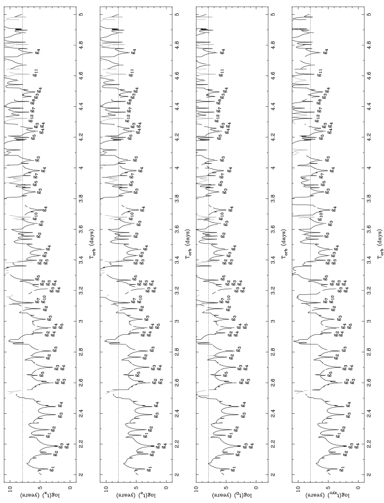
Figure 3: The logarithms of the time scales $t_{a}$, $t_{e}$, $t_{\Omega}$, and $t_{\rm syn}$ as functions of the orbital period for the $5\,M_{\odot}$ ZAMS model and for an orbital eccentricity $e=0.5$. The black lines correspond to orbital periods at which $da/dt<0$, $de/dt<0$, $d\Omega/dt>0$, and $[1/(\Omega-n)][d(\Omega-n)/dt]<0$, and the grey lines to orbital periods at which $da/dt>0$, $de/dt>0$, $d\Omega/dt<0$, and $[1/(\Omega-n)][d(\Omega-n)/dt]>0$. The dotted horizontal line represents the logarithm of the star’s nuclear time scale.

With the exception of the shortest orbital periods considered, the time scales for the relative rates of secular change of the orbital elements and the star’s rotational angular velocity are mostly longer than the star’s nuclear time scale, in accordance with the results of earlier investigations (e.g., Savonije & Papaloizou, 1983). The shortest time scales found for the relative rates of secular change are about five orders of magnitude smaller than the nuclear time scale. With regard to the synchronisation of the star’s rotation with the orbital motion of the companion, the time scales found are generally shorter than the time scales associated with the relative rates of secular change of the orbital eccentricity. Synchronisation of the star’s rotation with the orbital motion of the companion at the periastron of its relative orbit can therefore be expected to occur before the circularisation of the orbit. A similar conclusion was reached by Zahn (1977) for low-frequency dynamic tides, after averaging over the effects of resonances.

When the orbital period becomes larger, nonadiabatic resonant dynamic tides have a decreasing influence on the time scales for the relative rates of secular change of the orbital elements and the star’s angular velocity. The underlying reason is the rapid decrease of the quantity $H_{2,N}$ for higher-order $g^{+}$-modes, which are the relevant modes for resonances of dynamic tides in close binaries with longer orbital periods (see also Paper I).

On the basis of these results, we suggest that nonadiabatic resonant dynamic tides may be an efficient mechanism for the circularisation of orbits in close X-ray binaries, especially when the orbital period is short. X-ray binaries are thought to have initially highly eccentric orbits as a result of the supernova explosion which generates the compact star. However, the orbits of several X-ray binaries with short orbital periods have been reported to be circular. Two examples are the X-ray binaries Cen X-3 and SMC X-1. The orbital period of the system Cen X-3 is 2.1 days, and that of the system SMC X-1 3.9 days (Verbunt & Van den Heuvel, 1995). For close binaries with such short orbital periods and highly eccentric orbits, resonances of dynamic tides with low-order $g^{+}$-modes are quite possible.

8 Concluding remarks

We have studied the effects of nonadiabatic resonant dynamic tides in a component of a close binary on the orbital elements and on the star’s axial rotation. The companion is considered to move in a fixed Keplerian orbit, and the star is supposed to rotate uniformly around an axis perpendicular to the orbital plane, but the effects of the centrifugal force and the Coriolis force are neglected. The relative difference between the frequency imposed by the companion and the star’s eigenfrequency is assumed to be of the order of the ratio of the tidal force to the gravity at the star’s equator. Furthermore, the nonadiabatic effects are considered to be of the same order of magnitude at least in some region near the star’s surface.

We have derived semi-analytical solutions for the linear, nonadiabatic resonant dynamic tides by applying a two-time variable expansion procedure, in which the ratio of the tidal force to the gravity at the star’s equator is adopted as the small expansion parameter. In this perturbation method, the nonadiabatic effects are evaluated in the quasi-isentropic approximation. At the lowest order of approximation, the resonant dynamic tide corresponds to the free oscillation mode involved in the resonance. This conclusion is similar to the conclusion reached by Smeyers et al. (1998) for resonant dynamic tides treated in the isentropic approximation.

Due to the nonadiabatic effects, the amplitude of the resonantly excited oscillation mode is reduced in comparison to the amplitude it reaches in the isentropic approximation. The magnitude of the reduction is determined by the ratio of the coefficient of vibrational stability to the eigenfrequency of the oscillation mode.

The main difference with the dominant solutions derived in the isentropic approximation is that the nonadiabatic effects induce a phase shift between the tidal displacement and the tide-generating potential. The magnitude and the sign of the phase shift depend on the coefficient of vibrational stability and on the relative difference between the forcing angular frequency and the eigenfrequency of the oscillation mode involved in the resonance. The tidal displacement field lags behind the tide-generating potential when the star is vibrationally stable with respect to the oscillation mode, whereas it precedes the tide-generating potential when the star is vibrationally unstable with respect to the oscillation mode.

The phase shift leads to variations of the semi-major axis and the eccentricity of the companion’s relative orbit, in addition to the variation of the longitude of the periastron already found in the isentropic approximation of a resonant dynamic tide. The contributions to the relative rates of secular change of the semi-major axis and the orbital eccentricity are determined by Eqs. (46) and (47) and are of the order of $\left(R_{1}/a\right)^{7/2}$, which is much larger than the order of $\left(R_{1}/a\right)^{21/2}$ derived by Zahn (1977) for the limiting case of dynamic tides with small frequencies.

As well because of the phase shift, the companion exerts a torque on the tidally distorted star, which is normal to the orbital plane. The average value of the torque is given by Eq. (57). For nonaxisymmetric resonant dynamic tides, angular momentum is exchanged between the orbital motion and the star’s rotation. On the assumption that the star rotates as a rigid body, the relative rate of secular change of the angular velocity due to a resonant dynamic tide is determined by Eq. (64) and is of the order of $\left(R_{1}/a\right)^{3/2}$, which is also considerably larger than the order of $\left(R_{1}/a\right)^{17/2}$ derived by Zahn (1977) for the limiting case of dynamic tides with small frequencies.

We have applied our results to resonances of dynamic tides with second-degree, lower-order $g^{+}$-modes in a $5\,M_{\odot}$ zero-age main sequence stellar model consisting of a convective core and a radiative envelope. For the orbital eccentricity $e=0.5$, numerous resonances of dynamic tides with $g^{+}$-modes may occur in the range of orbital periods from 2 to 5 days. At several orbital periods, even resonances with two or more $g^{+}$-modes may take place.

Since the quasi-isentropic approximation led to inadequate results for the coefficient of vibrational stability, we passed on to the linear growth rates determined within the framework of a fully nonadiabatic analysis.

Relative to the resonances, we have determined time scales associated with the rates of secular change of the semi-major axis, the orbital eccentricity, and the star’s rotational angular velocity. The shortest time scales are found for the shortest orbital periods and for resonances with the lowest-order $g^{+}$-modes. They are about five orders of magnitude smaller than the star’s nuclear time scale. The time scales for synchronisation of the star’s rotation with the companion’s orbital motion at the periastron in the relative orbit are generally shorter than the time scales for circularisation of the orbit.

Because of the shortness of the time scales, the system may be expected to rapidly evolve away from any resonance between a dynamic tide and a free oscillation mode, so that only a limited amount of angular momentum can be exchanged between the star’s rotation and the orbital motion of the companion. However, Witte & Savonije (1999b, 2001) have shown that when both stellar and orbital evolution are taken into account, a dynamic tide can easily become locked in a resonance for a prolonged period of time. In these circumstances, the exchange of angular momentum might be sustained throughout the locking of the resonance.

For conclusion, in components of close binaries with short orbital periods and highly eccentric orbits, various resonant dynamic tides can be excited which, through their nonadiabatic character, may act as an efficient mechanism for the synchronisation of the rotation and the circularisation of the orbital motion of stellar components in time scales shorter than their nuclear time scales.

Appendix A Resonant dynamic tides within a fully nonadiabatic framework

In this appendix, we briefly describe how the lowest-order solution for a nonadiabatic resonant dynamic tide can be derived within a fully nonadiabatic framework.

Following Van Hoolst (1994), we express the equations that govern linear, nonadiabatic stellar oscillations in the form of a first-order, linear differential equation in the vector ${\@vec{z}}=(\@vec{\xi},\partial\@vec{\xi}/\partial t,\delta S)$, where $\@vec{\xi}$ is the Lagrangian displacement, and $\delta S$ the Lagrangian perturbation of the entropy. Adding the tidal force exerted by a companion star, one has

$${\partial{\bf z}\over\partial t}=M{\bf z}+\@vec{N},$$ (67)

where $\@vec{N}=(0,-\varepsilon_{T}\nabla W,0)$, and $M$ is the integro-differential operator governing free nonadiabatic stellar oscillations as defined in Van Hoolst (1994). The vector ${\bf z}$ is expanded in terms of linear, nonadiabatic eigenvectors ${\bf e}_{n}$ as

$${\bf z}(t,{\bf r})=\sum_{n}a_{n}(t){\bf e}_{n}({\bf r}),$$ (68)

where the eigenvectors ${\bf e}_{n}$ depend on time by $\exp(\sigma_{n}t)$ and obey the equation

$$M{\bf e}_{n}=\sigma_{n}{\bf e}_{n}.$$ (69)

The complex angular frequency $\sigma_{n}$ can be expressed as

$$\sigma_{n}=\kappa_{n}+{\rm i}\Omega_{n},$$ (70)

where $\Omega_{n}$ is the oscillation frequency, and $\kappa_{n}$ the opposite of the linear growth rate.

In order to derive a first-order expression for resonant dynamic tides, we use a multiple time scales method (Nayfeh, 1973, 1981). Therefore, we introduce time variables $T_{0}$ and $T_{1}$ as

$$T_{0}=t,\,\,\,T_{1}=\varepsilon_{T}t,$$ (71)

and expand the amplitude $a_{S}(t)$ of the resonant mode in terms of the small parameter $\varepsilon_{T}$ as

$$a_{S}=a_{S}^{(0)}+\varepsilon_{T}a_{S}^{(1)}.$$ (72)

In addition, we assume the linear growth rate to be small and of the order of $\varepsilon_{T}$. In contrast with the procedure followed in the quasi-isentropic treatment, we here do not consider the nonadiabatic effects to be small everywhere in the star.

The application of the method of the multiple time scales as described in Van Hoolst (1994) leads to an equation for the first-order real part of the eigenfunction that has the same form as Eq. (39), except for the fact that $\kappa_{\ell,N}$ now stands for the linear growth rate, and the fact that the factor $Q_{\ell,N}$ is defined in terms of the complex nonadiabatic eigenfunctions of the mode.

References

- Alexander (1973) Alexander M. E., 1973, Ap&SS 23, 459
- Cox (1980) Cox J. P., 1980, Theory of stellar pulsation, Research supported by the National Science Foundation Princeton, NJ, Princeton University Press
- Degryse et al. (1992) Degryse K., Noels A., Gabriel M., Waelkens C., Smeyers P., 1992, A&A 263, 137
- Dziembowski et al. (1993) Dziembowski W. A., Moskalik P., Pamyatnykh A. A., 1993, MNRAS 265, 588
- Gautschy & Saio (1993) Gautschy A., Saio H., 1993, MNRAS 262, 213
- Hut (1981) Hut P., 1981, A&A 99, 126
- Kevorkian & Cole (1981) Kevorkian J., Cole J. D., 1981, Perturbation Methods in Applied Mathematics, Springer-Verlag, New York
- Kevorkian & Cole (1996) Kevorkian J., Cole J. D., 1996, Multiple Scale and Singular Perturbation Methods, Springer-Verlag, New York
- Lai (1997) Lai D., 1997, ApJ 490, 847
- Ledoux & Walraven (1958) Ledoux P., Walraven T., 1958, ”Variable Stars” in Handbuch der Physik, edited by S. Flügge, Vol. 51, Springer-Verlag, Berlin
- Nayfeh (1973) Nayfeh A. H., 1973, Perturbation Methods, John Wiley and Sons, New York
- Nayfeh (1981) Nayfeh A. H., 1981, Introduction to perturbation techniques, John Wiley and Sons, New York
- Papaloizou & Savonije (1997) Papaloizou J. C. B., Savonije G. J., 1997, MNRAS 291, 651
- Polfliet & Smeyers (1990) Polfliet R., Smeyers P., 1990, A&A 237, 110
- Rocca (1989) Rocca A., 1989, A&A 213, 114
- Ruymaekers (1992) Ruymaekers E., 1992, A&A 259, 349
- Savonije & Papaloizou (1983) Savonije G. J., Papaloizou J. C. B., 1983, MNRAS 203, 581
- Savonije & Papaloizou (1984) Savonije G. J., Papaloizou J. C. B., 1984, MNRAS 207, 685
- Savonije & Papaloizou (1997) Savonije G. J., Papaloizou J. C. B., 1997, MNRAS 291, 633
- Savonije et al. (1995) Savonije G. J., Papaloizou J. C. B., Alberts F., 1995, MNRAS 277, 471
- Smeyers et al. (1991) Smeyers P., Van Hout M., Ruymaekers E., Polfliet R., 1991, A&A 248, 94
- Smeyers et al. (1998) Smeyers P., Willems B., Van Hoolst T., 1998, A&A 335, 622 (Paper I)
- Sterne (1960) Sterne T. E., 1960, An introduction to celestial mechanics, Interscience Publishers, London
- Stothers & Simon (1970) Stothers R., Simon N. R., 1970, ApJ 160, 1019
- Tassoul (1987) Tassoul J., 1987, ApJ 322, 856
- Terquem et al. (1998) Terquem C., Papaloizou J. C. B., Nelson R. P., Lin D. N. C., 1998, ApJ 502, 788
- Unno et al. (1989) Unno W., Osaki Y., Ando H., Saio H., Shibahashi H., 1989, Nonradial oscillations of stars, Nonradial oscillations of stars, Tokyo: University of Tokyo Press, 1989, 2nd ed.
- Van Hoolst (1994) Van Hoolst T., 1994, A&A 292, 471
- Verbunt & Van den Heuvel (1995) Verbunt F., Van den Heuvel E. P. J., 1995, in X-ray binaries, edited by W.H.G. Lewin, J. Van Paradijs, and E.P.J. Van den Heuvel, Cambridge University Press, Cambridge and New York, p. 457
- Willems (2000) Willems B., 2000, Contribution to the linear theory of dynamic tides and orbital evolution in close binaries, PhD Thesis, Katholieke Universiteit Leuven, Belgium
- Witte & Savonije (1999a) Witte M. G., Savonije G. J., 1999a, A&A 341, 842
- Witte & Savonije (1999b) Witte M. G., Savonije G. J., 1999b, A&A 350, 129
- Witte & Savonije (2001) Witte M. G., Savonije G. J., 2001, A&A 366, 840
- Zahn (1975) Zahn J. P., 1975, A&A 41, 329
- Zahn (1977) Zahn J. P., 1977, A&A 57, 383
- Zahn (1978) Zahn J. P., 1978, A&A 67, 162