Polarization of photospheric lines from turbulent dynamo simulations

Abstract

We employ the magnetic and velocity fields from turbulent dynamo simulations to synthesize the polarization of a typical photospheric line. The synthetic Stokes profiles have properties in common with those observed in the quiet Sun. The simulated magnetograms present a level of signal similar to that of the Inter-Network regions. Asymmetric Stokes $V$ profiles with two, three and more lobes appear in a natural way. The intensity profiles are broadened by the magnetic fields in fair agreement with observational limits. Furthermore, the Hanle depolarization signals of the Sr I $\lambda$4607 Å line turn out to be within the solar values. Differences between synthetic and observed polarized spectra can also be found. There is a shortage of Stokes $V$ asymmetries, that we attribute to a deficit of structuring in the magnetic and velocity fields from the simulations as compared to the Sun. This deficit may reflect the fact that the Reynolds numbers of the numerical data are still far from solar values. We consider the possibility that intense and tangled magnetic fields, like those in the simulations, exist in the Sun. This scenario has several important consequences. For example, less than 10% of the existing unsigned magnetic flux would be detected in present magnetograms. The existing flux would exceed by far that carried by active regions during the maximum of the solar cycle. Detecting these magnetic fields would involve improving the angular resolution, the techniques to interpret the polarization signals, and to a less extent, the polarimetric sensitivity.

1 Introduction

In the absence of gradients of velocity and magnetic field in the resolution element, the polarization emerging from an atmosphere must be either symmetric or antisymmetric with respect to the central wavelength of each spectral line (e.g., Unno 1956; Landi Degl’Innocenti & Landolfi 1983). The polarization observed in the solar photosphere does not show such symmetries. Asymmetric Stokes profiles arise from the quiet Sun (e.g., Sánchez Almeida et al. 1996; Sigwarth et al. 1999), from plages and network regions (e.g., Baur et al. 1981; Stenflo et al. 1984), as well as from sunspot penumbrae (e.g., Grigorjev & Katz 1972; Makita 1986; Sánchez Almeida & Lites 1992). The fact that such asymmetries are found even when observing at the limit of present resolution suggests that a rich structuring remains unresolved to the current observations.

Because asymmetries carry information on the spatially unresolved properties of the photospheric plasma, their study and correct interpretation offers a chance to overcome the limitations imposed by the angular resolution, and to retrieve information inaccessible to direct imaging. Indeed, such possibility has been exploited during the last decade, always relying on a considerable amount of modeling and assumptions. In broad terms, one can distinguish two approaches depending on the size of the unresolved structures that are responsible for the asymmetries.

The first approach assumes that the unresolved photospheric structures are actually on the verge of being resolved in broad-band images taken with the current instrumentation. The smallest detectable features are of the order of 0.2$\farcs$(or 150 km on the Sun); a size set by technical limitations of the present solar telescopes (e.g., Bonet 1999). Several models of this kind have been proposed to explain asymmetries in special cases like penumbrae, plage and network regions, and in the quiet Sun (e.g., Solanki & Montavon 1993; Grossmann-Doerth et al. 1988; Bellot Rubio et al. 1997; Steiner 2000). For example, Steiner (2000) invokes special thermal structures (temperature inversion) within magnetic regions in order to explain some extreme Stokes $V$ shapes frequently observed in the quiet Sun. The distinctive feature of this approach is that the proposed configurations (thermal, magnetic or kinetic) are specific to the case under study. The fact that asymmetries occur everywhere is therefore difficult to explain within this framework.

The second approach is more consonant with the ubiquity of the asymmetries in the polarization of photospheric lines. It assumes that the photospheric plasma is in a turbulent state and that small-scale structures both in velocity and magnetic field are present. Order of magnitude estimates for the magnetic and kinetic Reynolds numbers in the granulation indicate that the magnetic field could be structured on spatial scales as small as a few kilometers (e.g., Schüssler 1986). This picture is consistent with recent progress in dynamo theory suggesting that a substantial part of the magnetic field in the quiet Sun could be generated locally by dynamo action driven by the granular flows (Meneguzzi & Pouquet 1989; Petrovay & Szakaly 1993; Cattaneo 1999; Emonet & Cattaneo 2001). This second approach is also supported by certain observations indicating that the magnetic field is structured on spatial scales below the resolution limit of current telescopes (e.g., Berger & Title 1996; Berger et al. 1998; Sánchez Almeida 1998). Based on these premises, it is reasonable to think of the asymmetries as the result of observing magnetic fields that vary spatially on scales much smaller than the mean-free-path of the photons. Interpretations of Stokes profiles taking into account this very fine structuring of the atmosphere have been carried out for several years (Sánchez Almeida et al. 1996). The model atmospheres used to fit the observed profiles consist of a collection of magnetic and non-magnetic components, each containing mild gradients to comply with the height variations of the mean photosphere, but interleaved in such a way as to produce large gradients along the line-of-sight (Sánchez Almeida 1997). The appealing aspect of this approach is that asymmetries emerge spontaneously, and independently of the details of the model; arising from correlations between the magnetic and the velocity fields of the various components (e.g., asymmetries occur if, on average, downflowing elements have low magnetic field strength). It is known that atmospheres with micro-structure reproduce all kinds of Stokes profiles observed in the quiet Sun, including network and Inter-Network (IN) regions (Sánchez Almeida & Lites 2000; Socas-Navarro & Sánchez Almeida 2002). These MIcro-Structured Magnetic Atmospheres (MISMAs) portray a quiet Sun with large amounts of unsigned magnetic flux and very complex magnetic topology (very often two magnetic polarities coincide in a resolution element).

In the present paper we take advantage of recent developments in the numerical modeling of surface dynamos to understand the origin of asymmetries in the line polarization. We use the magnetic and velocity fields from a set of numerical data generated to study the interaction between thermally driven turbulent convection and magnetic fields (Cattaneo 1999; Emonet & Cattaneo 2001). Although these numerical simulations were not designed for a detailed description of the solar photosphere, the complexity and ubiquity of its fields recall in many respects the magnetic quiet Sun inferred from the observed asymmetries. Assuming a Milne-Eddington (ME) atmosphere for the thermodynamic variables we produce synthetic Stokes profiles. Thus, the asymmetries in the resulting profiles are directly related to the correlations between the velocity and the magnetic field that exist in the numerical data, but they are decoupled from the thermodynamic variables of the simulation. The comparison between the synthetic profiles and solar data shows that the synthetic spectra are frequently similar to the observed ones. Such agreement suggests that the simulation includes some of the ingredients that characterize the quiet Sun magnetic fields; in particular, the correlations between magnetic field and velocity at the smallest spatial scales. On the other hand, discrepancies between synthetic and observed Stokes profiles allow to identify missing ingredients and, consequently, to devise strategies to improve the simulations and the inversions. Finally, following Emonet & Cattaneo (2001), one can use the synthetic profiles to estimate the angular resolution required to determine the basic properties of the magnetic structures present in the numerical simulation. This angular resolution may be of relevance to decide the specifications of new solar instruments.

The work is organized as follows. The numerical data is briefly described in §2. The synthesis procedure is detailed in §3 and includes two subsections: in §3.1 we characterize the angular resolution of the model observations, and in §3.2 we calibrate the synthetic magnetograms. The main results of the synthesis are analyzed in §4: the variation of the apparent flux of the region depending on the sensitivity and spatial resolution of the observation (§4.1), the asymmetries of the Stokes $V$ profiles (§4.2), and the magnetic broadening of the intensity profiles (§4.3). Hanle depolarization signals to be expected for Sr I $\lambda$4607 Å are worked out in §5. §6 discusses the diameter of the ideal telescope needed to spatially resolve the simulations. Finally, the implications of the present work are discussed in §7.

2 Description of the set of MHD data

The numerical data set used in the present work is part of a series of numerical simulations to study the generation and interaction of magnetic fields with turbulent convection. The simulations are based on a idealized model describing a layer of incompressible (Boussinesq) fluid with constant kinematic viscosity $\nu$, thermal diffusivity $\kappa$ and magnetic diffusivity $\eta$. The boundary conditions are periodic in the horizontal directions, and impenetrable and stress free with constant temperature and zero horizontal magnetic field along the upper and lower boundaries of the computational domain. As is common in this kind of simulations, the unit of length is the vertical extent of the layer, the unit of time is the thermal diffusion time across that layer and the magnetic intensity is expressed as an equivalent Alfvén speed. With these units the particular dynamo solutions used below is defined by the following dimensionless parameters: aspect-ratio of the computational domain $10\times 10\times 1$, Rayleigh number $5\times 10^{5}$ and Prandtl numbers $\nu/\kappa=1$, $\nu/\eta=5$. The numerical resolution was $512\times 512\times 97$ collocation points. In this regime, the solution corresponds to a state of vigorous convective turbulence characterized by a kinetic and magnetic Reynolds numbers of ${\hbox{Re}}=200$ ${{\hbox{Re}}_{m}}\simeq 1000$, respectively. The resulting flow is strongly chaotic and acts as an efficient dynamo generating an intermittent magnetic field with no mean flux and a magnetic energy roughly 20% of the kinetic energy. For the present study, we use one time step of the dynamo evolution that is well into the statistically stationary regime. At this epoch, the rms velocity of the fluid is $u\approx 200$ with a corresponding turnover time of $1/100$. A more complete description of the simulation procedure, and further details about the numerical solutions can be found in Cattaneo (1999), Emonet & Cattaneo (2001) and Cattaneo et al. (2001).

3 Spectral synthesis

The numerical simulations described above were not designed specifically for spectral synthesis, rather to study dynamo action. In order to achieve the high magnetic Reynolds numbers (${{\hbox{Re}}_{m}}=1000$) necessary for dynamo action to manifest itself, and given finite computer resources ($10^{7}$–$10^{8}$ grid points), we found it necessary to resort to the Boussinesq approximation. The latter is valid provided that the vertical extent of the layer is much smaller than the pressure, density, and temperature scale heights (see e.g. Spiegel & Veronis 1960). As a consequence, the thermodynamic variables from the numerical solutions have modest variations across the layer, and cannot be used to calculate the opacity and source functions needed for the synthesis. Consequently, we address the synthesis problem ignoring the thermodynamic variables from the simulations, but keeping the variations in the velocity (${\bf u}$) and magnetic field (${\bf b}$). Although ${\bf u}$ and ${\bf b}$ are then decoupled from the density and temperature distributions, the resulting synthetic profiles are useful to study the properties of the emerging line polarization that depends, primarily, on the magnetic and velocity structure. In the remainder of this section we explain the process followed to generate the synthetic profiles.

The first step is to translate the dimensionless velocity and magnetic data of the simulations into units that are practical for the synthesis. The spatial scale is fixed by assuming that the typical size of one granule is about 1000 km. In the statistically stationary regime the computational domain is about 5 granules wide. Thus the horizontal size of the domain corresponds to 5000 km, with a corresponding grid resolution of approximately $10$ km in the horizontal, and $5$ km in the vertical. Magnetic field strengths $B$ and velocities $U$ readily follow from the energy equipartition arguments. $B$ and $U$ are proportional to the dimensionless magnetic strength $b$ and velocity $u$ through the factors $f_{u}$ and $f_{b}$,

$$B= f_{b}b,\qquad U= f_{u}u.$$ (1)

Equipartition between kinetic energy density and magnetic energy density is reached in dimensionless units when

$$b_{eq}^{2}=u_{eq}^{2},$$ (2)

or equivalently when

$$B_{eq}^{2}/(8\pi)=\rho U_{eq}^{2}/2\;,$$ (3)

$\rho$ being the density. The previous equation, together with equations (1) and (2), lead to

$$f_{b}=f_{u}(4\pi\rho)^{1/2}\;.$$ (4)

Thus, if one associates the rms speed $u\simeq 200$ with the rms velocity fluctuations observed in the solar granulation $U=2$ km s^-1 (e.g., Durrant 1982; Topka & Title 1991), then

$$f_{u}=10^{-2}\ {\rm km\ s}^{-1}\;,$$ (5)

and for a typical density at the base of the photosphere (3 $\times 10^{-7}$ g cm^-3; Maltby et al. 1986), equations (4) and (5) render

$$f_{b}\simeq 2\ {\rm G}\;.$$ (6)

Except for a few exploratory calculations described in §4.2 and §5, the scaling factors in equations (5) and (6) are used for the rest of the work. Notice that reasonable deviations from this scaling do no affect our results in a substantial way (a point addressed in §4).

Following our previous assumption, the absorption and emission terms of the radiative transfer equations (e.g., Beckers 1969; Wittmann 1974; Landi Degl’Innocenti 1976) are not based on the thermodynamic variables of the numerical data set. Instead, we resort to a Milne-Eddington (ME) synthesis which assumes a constant line absorption and a linear source function (e.g., Unno 1956; Landi Degl’Innocenti 1992). The ME assumption is routinely used for magnetic field diagnostics (e.g., Socas-Navarro 2001) since it yields an analytic expression for the emerging polarized spectrum that only depends on a few parameters. The analytic solution is used to fit observed spectra and retrieve information from them (e.g., Skumanich & Lites 1987). The ME synthesis hides all the unknown thermodynamic properties of the atmosphere in five parameters, namely, the line absorption coefficient, two parameters that define the (linear) source function, the damping coefficient, and the Doppler width. In our syntheses, we adopt the values characteristic of the Fe I line at $\lambda$6302.5 Å in the quiet Sun (Sánchez Almeida et al. 1996, Table 1, including a Doppler width of 40 mÅ or 1.9 km s^-1). This magnetically sensitive spectral line is often used for magnetic studies, including those of the Advanced Stokes Polarimeter (Elmore et al. 1992). Working with the same line allows us to compare our results directly with its observations. The use of observed ME thermodynamic parameters to represent the synthetic line provides realism to the part of the synthesis that we do not obtain directly from the numerical simulation. The emerging spectra will have the observed equivalent widths, line widths, etc.

The standard ME assumption considers an atmosphere having a uniform magnetic field (e.g., Unno 1956; Landi Degl’Innocenti 1992). Such assumption is clearly at odds with our numerical data in which the magnetic diffusive scale is of the order of $500\times{{\hbox{Re}}_{m}}^{-1/2}$ km $\simeq 15$ km, i.e., three grid points in the vertical direction. The field is therefore not constant over the range of heights where the typical photospheric lines are formed (say 100 km). A realistic spectral line synthesis would have to take into account the contributions from many layers in the simulation. The brute-force approach would be to assign an optical depth to each horizontal plane in the simulation and then synthesizing the spectrum by direct numerical integration of the radiative transfer equations for polarized light. Here, instead, we resort to a different strategy that a) is simpler and much faster, b) reduces the number of free parameters of the synthesis (no need to specify the optical depths of all the different planes of the atmosphere) and, c) produces spectra very close to those obtained by the brute-force approach. We employ a multi-component ME atmosphere, as defined by Sánchez Almeida et al. (1996; §2.1). We assume that not all individual planes of the simulation contribute to the emerging spectrum, and consider only a sub-set whose thickness is of the order of the photon mean-free-path. We take into account that the planes are optically thin so that the emerging spectrum depends only on the average along the line-of-sight of the emission and the absorption (the so-called MISMA approximation; Sánchez Almeida et al. 1996). As argued below, these assumptions are not unreasonable, and reduce the radiative transfer calculation to deciding how many planes contribute to the emerging spectrum. Subsequently, the average absorption matrix is computed, and used jointly with the analytic solution for the regular ME synthesis (Sánchez Almeida et al. 1996).

In our case we choose the 21 uppermost planes of the simulation, excluding the upper boundary. According to the scaling described in the previous paragraph, this corresponds to approximately 100 km in the atmosphere, a typical range for the formation of a photospheric line. We further assume that the numerical simulation is placed at disk center, i.e., with the line-of-sight along the vertical direction.

Since the individual planes of the simulation are indeed optically thin (5 km), using the average emission and absorption instead of solving the full radiative transfer should be a good approximation. We checked this assumption by comparing spectra computed by direct integration of the radiative transfer equation with those resulting from our approximation. Figure 1 contains one example. The full synthesis is performed assuming the 21 different planes of the ME synthesis to be equi-spaced in and spanning from $\log\tau=0$ to $\log\tau=-1$. (The symbol $\tau$ stands for the continuum optical depth.) This layer is periodically repeated to complete the atmosphere from $\log\tau=10$ to $\log\tau=-3$. The synthesis of 1000 randomly chosen spectra shows relative differences between the two kinds of syntheses of only a few per cent. This deviation is negligible for the analysis that we carry out in the present work. The choice of number of planes to be used for the spectral synthesis is a more delicate matter. Using 26 instead of 21 planes we find differences between spectra of up to 25%. These differences are due to the strong variability of the magnetic conditions, an uncertainty that also affects any other way of synthesizing the spectra. For example, in the case of the brute-force approach the signals depend on the optical depths arbitrarily assigned to each plane of the numerical data.

3.1 Spatial resolution: seeing and telescope diameter

Studying the consequences of observing the simulations with a finite spatial resolution is one of the key objectives of the present work. We use the term seeing to denote all the effects that may reduce the spatial resolution (from genuine seeing to optical aberrations of the instruments). Here the effects of seeing are modeled by smearing the 2D maps of the Stokes profiles with Gaussian functions. Note that the 2D convolution is carried out at each individual wavelength of each Stokes parameter. The amount of smearing is characterized by the FWHM (Full Width Half Maximum) of the Gaussian function. We take this particular point spread function for the sake of simplicity, however, it accurately describes long-integration-time atmospheric seeing (e.g, Roddier 1981, §4.5). In one of the sections (§6), we measure seeing in terms of the diameter, $D$, of an ideal telescope that provides a given angular resolution. Considering that the Airy disk of an ideal telescope has a FWHM $\simeq\lambda/D$, then

$$D=13\ {\rm cm\ (\lambda/6302)\ (FWHM/725)^{-1}},$$ (7)

where FWHM is expressed in km and $\lambda$ in Å. We have used a scale of 725 km/″, corresponding to our target at 1 AU.

3.2 Longitudinal Magnetograms

Longitudinal magnetograms are images showing the degree of circular polarization in the flank of a spectral line (e.g., Babcock 1953; Landi Degl’Innocenti 1992; Keller et al. 1994). They can be produced using relatively simple and compact instruments and therefore have been widely used in solar magnetic field studies. A significant fraction of what we know about quiet Sun magnetic fields has been derived from them (e.g., Wang et al. 1995, and references therein). Longitudinal magnetograms are usually calibrated in units of magnetic field strength (G). Since we wish to compare the polarization signals with observed magnetograms, calibrated magnetograms must be prepared out of the synthetic Stokes profiles. We follow a procedure that mimics the observational process. First, the circular polarization signals are averaged in wavelength, this is because magnetograms are often obtained through a rather broad color filter. We employ a running box filter, 100 mÅ wide, centered in the blue wing of the line at 50 mÅ from the line center. (These values are comparable to those employed in real measurements; e.g., Yi & Engvold 1993; Berger & Title 2001.) Then the wavelength averaged circular polarization signal $V_{a}$ is calibrated to yield the so-called longitudinal magnetic flux density $B_{\rm los}$, i.e.,

$$B_{\rm los}=C_{\rm cal}\thinspace V_{a}.$$ (8)

The calibration constant $C_{\rm cal}$ is evaluated using the magnetograph equation and the properties of the line in which the magnetograph operates; explicitly,

$$C_{\rm cal}^{-1}=-c\lambda_{0}^{2}g_{\rm eff}{{dI_{a}}\over{d\lambda}}.$$ (9)

Here, the symbol $\lambda_{0}$ stands for the central wavelength of the line, $g_{eff}$ is the effective Landé factor, and $I_{a}$ corresponds to the intensity profile smeared with the same color filter used to produce $V_{a}$. The constant $c$ equals 4.67 $\times~{}10^{-13}$ Å^-1 G^-1. For the atomic parameters of Fe I $\lambda$6302.5 Å, and using the mean Stokes $I$ profile over a complete snapshot, we find $C_{\rm cal}\simeq~{}5850$ G when $V_{a}$ is given in units of the continuum intensity. This synthetic calibration constant is in good agreement with the values that can be found in the literature for this line (e.g., Yi & Engvold 1993; Lites et al. 1994; Socas-Navarro & Sánchez Almeida 2002).

With several additional simplifying assumptions, it can be shown that

$$B_{\rm los}=\int_{S}B_{z}dS\Big{/}\int_{S}dS,$$ (10)

where the integrals extend to the resolution element $S$, and $B_{z}$ is the component of the magnetic field vector pointing towards the observer. This identity provides the rationale to denote magnetogram signals as longitudinal magnetic flux densities. (According to equation [10], $B_{\rm los}$ represents the magnetic flux per unit area.)

4 Results

In this section we analyze the synthesis of the 512 $\times$ 512 Stokes spectra calculated from the dynamo simulation described in §2. We only use the numerical solution at one instant since the purpose of the work is to study the kind of spectra characterizing the stationary state of the simulation (studies of the time dependent behavior is deferred for later). We place the simulation at the solar disk center so that the vertical direction follows the line-of-sight.

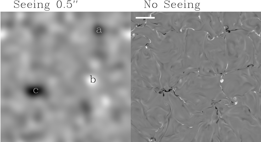
Figure 2: Magnetogram of the snapshot of the numerical simulation analyzed in the work. It shows both the original one at full resolution (right), as well as the result of smearing the magnetogram with a 0$\farcs$5 seeing (left). The white gauge indicates 1″ on the Sun. The labels $a$, $b$ and $c$ point out three entities that may be identified as single magnetic concentrations in the 0$\farcs$5 seeing magnetogram. The scale of grays of the two magnetograms is independent since the seeing diluted signals (left) would remain almost unnoticed if scaled to those in the original magnetogram (right).

Figure 2 shows the magnetogram that results when applying equation (8) to the synthetic Stokes $V$ spectra (right panel). The effect of observing with a 0$\farcs$5 seeing – representative of the best angular resolution achieved at present (e.g., Berger & Title 2001), is also shown on the left panel. Ignoring the underlying substructure, an observer would identify a number of magnetic concentrations in the smeared magnetogram (e.g., points $a$, $b$ and $c$). However, these are difficult to associate with single structures once the underlying substructure is acknowledged. Rather, the points with enhanced signal in the 0$\farcs$5 magnetogram represent locations where the convective flows are continuously advecting magnetized plasma to balance the plasma that constantly disappears in the downdrafts (see also § 3.2 in Emonet & Cattaneo 2001). The fact that the residual polarization signal shows up suggests the presence of a large-scale structure of the advecting velocity. Indeed, detailed analysis of the numerical data reveals the existence of a mesogranular flow (Cattaneo et al. 2001).

Except for a few test calculations in §4.2, the spectra discussed in this section correspond to a scaling of the dimensionless magnetic field and velocity given by equations (5) and (6). However, syntheses using $f_{u}=0.02$ km s^-1 and $f_{b}=2.5$ G were also tried. We found that the degree of circular polarization increases linearly as $f_{b}$, whereas a larger $f_{u}$ enhances the line asymmetries. On the other hand, the kind of general trends and properties that we analyze here do not depend on the precise value of the scale factors.

4.1 Flux density versus angular resolution

The amount of magnetic flux and energy in the numerical data is far larger than that detected in the Sun as IN fields. This difference can be understood as the result of two important factors that hinder the detection of the weak signals emerging from the simulation. First, the magnetic fields are highly disorganized so that the polarization signals tend to cancel as the angular resolution deteriorate (Emonet & Cattaneo 2001). Second, most synthetic signals are extremely low, i.e. at and below the sensitivity of the present instrumentation. Consequently a large fraction could not be detected at present. In this section we use our synthetic lines to explore these effects. We find that once realistic angular resolution and sensitivity are taken into account, the simulations are in good agreement with the observations.

Figure 3 shows the mean unsigned signal in the magnetogram of Figure 2 as a function of the seeing (i.e., mean $|B_{\rm los}|$ over the snapshot versus FWHM of seeing). We consider various sensitivities of the magnetograph: moderate (20 G), good (5 G) and very good (0.5 G). We account for the limited sensitivity by setting to zero all those points in the smeared magnetogram where the signal is below the hypothetical observational threshold. Figures 3b is identical to Figure 3a except that it has been normalized to the mean longitudinal field in the simulation (i.e., mean $|B_{z}|\simeq 51$ G, where the average considers all the points of the simulation that we use). According to the standard interpretation (equation [10]), this is the parameter that one retrieves from a magnetogram. The normalization helps visualizing the fraction of real signal that remains in the magnetogram for a given angular resolution and sensitivity. There are several features in these two figures that deserve comment.

Even with perfect sensitivity and maximum angular resolution, one detects only 80 % of the existing flux. The cancellation is mostly due to the averaging along the line-of-sight caused by the radiative transfer. At maximum angular resolution, the flux in the magnetogram depends little on the sensitivity since most of the signals exceed 20 G.

The decrease in signal strength as the angular resolution deteriorate is severe. For the typical 1″ angular resolution, the detectable signals are only 10 % of the original ones (Fig. 3b). This estimate is optimistic since it holds true if the sensitivity is good; should the latter be moderate, only traces of the original signals remain (1% for 20 G sensitivity).

Figure 3a includes values for solar IN magnetic flux densities observed by various authors. The level of detected flux density agrees well with the predictions of the simulations once the angular resolution has been taken into account. Note that the observed flux densities are more than a factor of ten smaller than the signals in the original magnetogram. We should not overemphasize the agreement, since the observational points are rather uncertain (they come from inhomogeneous sources, with different sensitivities and based on disparate techniques: see below). However, two conclusions can be drawn. First, intense yet tangled magnetic fields like those in the numerical simulation are compatible with the present solar observations. Second, if our spatially fully resolved synthetic spectra were emitted by the Sun, they would produce the degree of polarization that we detect on the Sun with the present instrumentation.

The observations presented in Figure 3a required transformation from the numbers quoted in the original works to the quantities plotted in the figure. Here we briefly describe these transformations for the sake of completeness. (The symbols accompanying the citations correspond to those used in Fig. 3a.) Socas-Navarro & Sánchez Almeida (2002; bullet sign $\bullet$) deduce 10 G mean flux density for the quiet Sun fields, however, they mention that the apparent flux density decreases by a factor 2.4 if it is estimated from magnetograms. This renders 4.2 G for a 1″ angular resolution, a figure derived from the cut off frequency in the Fourier domain of the continuum intensity image (Sánchez Almeida & Lites 2000). The same procedure is used to estimate the angular resolution of the spectra in Collados (2001; square $\Box$). The mean flux density, 3.4 G, has been directly provided by the author. Wang et al. (1995; asterisk $\ast$) point out, explicitly, a 1.65 G flux density for their angular resolution of 2″. Stolpe & Kneer (2000; times sign $\times$) find some 3.5 G mean flux density (private communication), to which we associate an angular resolution of two pixels or 1$\farcs$4. Lin & Rimmele (1999; triangle $\bigtriangleup$) do not directly give a mean flux density for their measurements. However, their Figure 3 contains the magnetic fluxes of individual measurements, and the authors provide the scale factor between the magnetic flux and the magnetic flux density ($5\times 10^{15}$ Mx G^-1). With this conversion, the mean flux density of these observations is about 4 G. The magnetic features occupy 68 % of the surface, since the rest remains below the sensitivity threshold. Consequently, the mean flux density over the whole surface results 0.68 $\times~{}4$ G. Grossmann-Doerth et al. (1996, Fig. 1; plus sign $+$) provide the distribution of Stokes $V$ Fe I $\lambda$5250 Å signals found in the quiet Sun, being the average signal about $2\times 10^{-3}$ (in units of the continuum intensity). The authors also point out a calibration constant from Stokes $V$ signal to flux density. It gives 2 G for the mean observed signal. Since these signals fill 40% of the solar surface, the mean flux density is about 0.8 G. We assign to these data an angular resolution twice the sampling interval (some 2$\farcs$3). Finally, Domínguez Cerdeña et al. (2002; diamond $\diamond$) have recently found 17 G mean flux density in a 0$\farcs$5 angular resolution magnetogram taken with Fe I $\lambda$6302.5 Å.

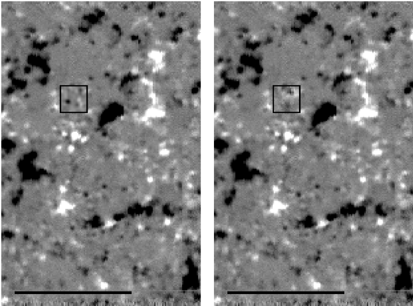
Figure 4: Synthetic magnetogram embedded in the real magnetogram of a quiet Sun region: inset within a box in the left image. The right image shows the original magnetogram, including the box for reference. The bar in the bottom corresponds to 25 000 km on the Sun, i.e., the linear dimension of a typical network cell. Note how the synthetic magnetogram fits in smoothly within the real magnetogram. It produces the right polarization for IN fields and it also has the proper spatial scales.

Figure 4 provides a different illustration of the similarities between the synthetic magnetogram and the real Sun. It shows a real magnetogram of the quiet Sun obtained in the blue wing of Fe I $\lambda$6302.5 Å  (Sánchez Almeida & Lites 2000, Fig. 1), i.e., using the observational setup that we have tried to reproduce (see §3.2). A patch of the real magnetogram with the size of the numerical simulation has been replaced with the synthetic one (Fig. 4 left). Except for the location of the inset, which we place in an IN region, we have not used free parameters to produce the combined magnetogram. The angular resolution has been chosen to match the observation (1″), whereas the degree of polarization comes directly from the synthesis. Despite the absence of fine-tuning, it turns out to be extremely difficult to distinguish the magnetogram with the artificial inset (Fig. 4 left) from the real one (Fig. 4 right). In other words, the synthetic magnetogram contains structure with a spatial distribution similar to the observed one, and with a degree of polarization which fits within the observed range.

4.2 Asymmetries of the Stokes $V$ profiles

In the absence of gradients of magnetic and velocity fields within the resolution element, the Stokes profiles have to obey well defined symmetries (see §1). This kind of symmetries are never found in the quiet Sun, instead profiles frequently show extreme asymmetries (Sánchez Almeida et al. 1996; Grossmann-Doerth et al. 1996; Sigwarth et al. 1999). Because the magnetic field in the numerical simulation has a highly intermittent structure (Cattaneo 1999; Emonet & Cattaneo 2001), we expected the resulting synthetic Stokes profiles to be asymmetric. In the following, we compare our synthetic profiles with observed ones and study in a statistical sense their differences and similarities. We proceed by first classifying the types of Stokes $V$ profiles produced by the simulation. The $2.6\times 10^{5}$ Stokes $V$ profiles in the snapshot were assorted using a cluster analysis algorithm identical to that employed with real data by Sánchez Almeida & Lites (2000; §3.2). The procedure identifies and groups profiles with similar shape, irrespective of their degree of polarization and polarity, since it employs Stokes $V$ profiles normalized to the largest blue peak (see Sánchez Almeida & Lites 2000 for details).

The classification is summarized in Figure 5. For each different class, the averaged Stokes $V$ profile over the ensemble is plotted. The mean is taken after each individual profile has been multiplied by the sign of its largest blue peak. This avoids cancellation of different polarities. The mean profiles are numbered (upper left corner in each panel) according to the percentage of profiles in the simulation that are elements of their class, with #0 being the most probable and #17 the least probable. The probability to find a profile of a given class is indicated in the upper right corner of each panel. Note the various possibilities. From virtually anti-symmetric Stokes $V$ (implying no asymmetry), to profiles with one (e.g., #11 and #13) or three lobes (e.g., #12 and #14). All these asymmetries are produced by gradients of magnetic and velocity fields along the line-of-sight. The peak polarization is considerable, some 1% in units of the continuum intensity. This has to be the case to yield the large flux density shown in Figure 3a for perfect angular resolution. Another detail worthwhile noting is the balance between the number of profiles having a large blue lobe and those whose principal lobe is the red one.

The line shapes in Figure 5 are difficult to compare with observed profiles since observations of the quiet Sun have much lower angular resolution. Figure 6 shows another classification having all the features explained above, except that the simulation data have been smeared with a 1″ seeing, typical of the real observations. First, the polarization signals are reduced by one order of magnitude with respect to the original profiles; compare them with those in Figure 5. Second, new more complicated line shapes have arisen as the result of the large spatial smearing (radiative transfer smoothes over only 100 km, whereas the spatial smearing does it over 725 $\times$ 725 km²). Stokes profiles having all these very asymmetric shapes are indeed observed in the real quiet Sun (see Sánchez Almeida et al. 1996, Fig. 12; Sigwarth et al. 1999, Fig. 7; Sánchez Almeida & Lites 2000, Fig. 4, 5 and 6; Sigwarth 2001, Fig. 4). This qualitative agreement is again a notable feature of the simulation, since there was no obvious a priori reason to expect it.

However, despite such general qualitative agreement, one can find quantitative differences between the synthetic and the observed profiles. As it happens with the fully resolved profiles (Fig. 5), the number of synthetic profiles having a principal blue lobe and those with a principal red lobe is similar (e.g., the pairs #12 and #18; #31 and #34; #33 and #35). Such balance is not present among the observed profiles, where the blue lobe usually dominates (e.g., Sánchez Almeida & Lites 2000, Fig. 4; Sigwarth et al. 1999, Fig. 12). Another qualitative difference with observations concerns the profiles that are most frequently obtained in the simulation. They show almost no asymmetry (see classes #0 to #7). Contrariwise, the observational counterpart have a well defined asymmetry characterized by a large blue lobe (similar to those observed in plage and enhanced network regions). This lack of significant asymmetry can be traced back to the original syntheses (Fig. 5, classes #0 to #4), and therefore to the variations along the line-of-sight of the magnetic field and velocity. The probable cause is discussed in the next paragraph.

Figure 7 summarizes the kind of variations along the line-of-sight existing in the numerical simulation. Several definitions are required before it can be interpreted. The variations are described using standard statistical parameters, namely, the line-of-sight mean value $\overline{f}_{ij}$, the line-of-sight standard deviation $\overline{\delta f}_{ij}$, and the line-of-sight correlation coefficient $\overline{(fg)}_{ij}$,

$$\overline{f}_{ij}=n_{z}^{-1}\sum_{k=1}^{n_{z}}f_{ijk},$$

$$\overline{\delta f}_{ij}=\Bigl{[}\overline{(f_{ijk}-\overline{f}_{ij})^{2}}\Bigr{]}^{1/2},$$ (11)

$$\overline{(fg)}_{ij}=\bigl{[}\overline{(f_{ijk}-\overline{f}_{ij})(g_{ijk}-\overline{g}_{ij})}\bigr{]}\Big{/}\bigl{[}\overline{\delta f}_{ij}~{}\overline{\delta g}_{ij}\bigr{]}.$$

The arrays $f_{ijk}$ and $g_{ijk}$ may represent any component of the fields, and their indexes vary according to the position in the horizontal plane ($i$ and $j$) and in the vertical direction ($k$). The symbol $n_{z}$ stands for the number of grid points in the vertical direction. We should bear in mind that the line-of-sight averages defined in equations (11) depend on the horizontal coordinates. We need to characterize the typical properties of these line-of-sight mean values for each range of mean longitudinal magnetic field strength. For this purpose we define the average $\langle\overline{h}\rangle$ and the dispersion $\Delta\overline{h}$ of the quantity $\overline{h}$ among all those points in the simulation with a given line-of-sight mean longitudinal magnetic field $\xi$, i.e.,

$$\langle\overline{h}\rangle(\xi)=n_{s}^{-1}\sum_{i=1}^{n_{x}}\sum_{j=1}^{n_{y}}\overline{h}_{ij}\ P(\xi,i,j),$$ (12)

$$\Delta\overline{h}(\xi)=\Big{[}n_{s}^{-1}\sum_{i=1}^{n_{x}}\sum_{j=1}^{n_{y}}\Big{(}\overline{h}_{ij}-\langle\overline{h}\rangle(\xi)\Big{)}^{2}\ P(\xi,i,j)\Big{]}^{1/2},$$ (13)

with

$$P(\xi,i,j)=\cases{1,&if $\big{|}\xi-|\overline{B_{z}}|_{ij}\big{|}<\epsilon/2$,\cr 0,&otherwise,}$$ (14)

and

$$n_{s}=\sum_{i=1}^{n_{x}}\sum_{j=1}^{n_{y}}P(\xi,i,j).$$ (15)

Note that the symbol $\overline{h}$ may represent any of the statistical parameters in equation (11) ($\overline{f}$, $\overline{\delta f}$ or $\overline{(fg)}$), and $n_{x}$ and $n_{y}$ correspond to the grid points in the two horizontal directions. The bin size $\epsilon$ has to be chosen to guarantee having enough points per bin. Following these definitions, we can now interpret Figure 7. The different quantities represented are plotted as function of the line-of-sight mean magnetic field.

The first panel in Figure 7 shows the variation of $\langle\overline{U_{z}}\rangle$ and $\langle\overline{\delta U_{z}}\rangle$. The limited dispersion of the vertical velocities provides an explanation for the predominance of profiles with small asymmetries. The dispersion must be of the order of the line width to produce a substantial modification of the line shape. The typical standard deviation of the vertical velocities along the line-of-sight turns out to be between 0.2 and 0.3 km s^-1 ($\langle\overline{\delta U_{z}}\rangle$, Fig. 7a, the solid line), whereas the line widths are of the order of 2 km s^-1 (see §3). The magnetic field itself is probably not responsible for the moderate asymmetries since its variations along the line-of-sight are large. For example, Figure 7b shows the standard deviation of the mean longitudinal magnetic field $\langle\overline{\delta B_{z}}\rangle$, which is frequently larger than the absolute value of $\overline{B_{z}}$. In fact, the variations of the longitudinal magnetic fields are so important that $B_{z}$ very often changes sign along the line-of-sight (Fig. 7c). Note that none of these statements on large magnetic field gradients apply to the intrinsically strong fields, a case discussed separately in the next paragraph. Above, say, 200 G, the variations of field strength are mild and the longitudinal field maintains a constant sign along the line-of-sight (Figs. 7b and 7c). Concerning the balance between the number of asymmetries towards the blue and towards the red in Figures 5 and 6, it is probably due to the lack of a definite sign for the correlation between magnetic field and velocity. Works on the asymmetries in plage and network regions repeatedly indicate the need for a negative correlation to account for the observed preponderance of the Stokes $V$ blue lobe, explicitly,

$$\overline{(U_{z}|B_{z}|)}<0,$$ (16)

(see, e.g., Solanki & Pahlke 1988; Sánchez Almeida et al. 1988; Sánchez Almeida et al. 1989; Grossmann-Doerth et al. 1988; Grossmann-Doerth et al. 1989; Sánchez Almeida 1998). Such condition is satisfied when downflows and magnetic fields are spatially separated, i.e., when the strongest downflows tend to occur in weakly magnetized plasma. (Note that $U_{z}>0$ corresponds to downflows.) One can see in Figure 7d that the correlation between $|B_{z}|$ and $U_{z}$ has a well defined negative value only for the largest field strengths. Since theses points represent a small fraction of the synthetic profiles, they contribute very little to the classification in Figure 5 which, consequently, shows no obvious preference for a blue asymmetry.

Those patches in the simulation with the largest field strength show a clear negative correlation fulfilling the criterion in equation (16) (see Fig. 7d). Do they produce the observed Stokes $V$ profiles with a main blue lobe? They do not, since the asymmetry of the profiles emerging from concentrations of intense field strength are minimal. This fact can be understood using Figures 7a and 7b, which reveal gradients of both magnetic field and velocity too small for the requirements described in the previous paragraph. Despite this apparent disagreement, the key ingredients to yield the right shapes are already present in the simulation. If one artificially increases the gradients of magnetic field and velocity already existing in the simulation, large asymmetries similar to the observed ones automatically show up. Figure 8 contains synthetic profiles emerging from the three more intense magnetic concentrations in the snapshot (labeled as $a$, $b$ and $c$ in Fig. 2, left). Note that they already have the Stokes $V$ asymmetries that characterizes network and IN regions. (Figure 8d includes one of these observed Stokes $V$ profiles for reference, namely, one network profile in Sánchez Almeida & Lites 2000). In order to produce theses new synthetic profiles with enhanced asymmetries, we increased the intensity of the flow with respect to the scaling in §3 by using $f_{u}=0.04$. In addition, we increased the variations of magnetic field strength by averaging all the absorption and emission over 0$\farcs$5 of the simulation (i.e., over all the points in a box of this size). The qualitative agreement between synthetic and real profiles is remarkable.

The above considerations lead to an interesting question. How should the numerical simulations be modified in order to produce asymmetries closer to the observed ones? First, the dispersion of velocities at the smallest scales must be increased, which implies a decrease in the kinematic viscosity. Second, magnetic and non-magnetic regions should be even more intermittent to strengthen the correlation (16). This can be achieved by decreasing the magnetic diffusivity, which would both increase the tangling of magnetic field lines and the dispersion of field strengths existing in the intense concentrations.

4.3 Broadening of the Intensity profiles

One of the observational constraints on the existence of a complex and tangled magnetic field in the solar photosphere comes from the work by Stenflo & Lindegren (1977) (see also Unno 1959; Stenflo 1982). If a tangled magnetic field exist, it has to broaden the spectral lines of the solar spectrum according to their magnetic sensitivities (i.e., according to their effective Landé factors). All other things being the same, those with larger sensitivity should be slightly broader. Stenflo & Lindegren (1977) looked for such effect in the solar unpolarized spectrum with no success. From the error budget of the measurement the authors set an upper limit to the field strength of the existing fields (Stenflo & Lindegren 1977, equation [12]),

$$B_{\rm app}\leq 140\ {\rm G}.$$ (17)

In this section we analyze if the magnetic fields in the simulations produce line broadenings compatible with such observational upper limit. This exercise allows to address the question of whether magnetic fields as intense as those in the simulation may exist on the Sun, and still remain below the present observational detection limit. We already know that the degree of circular polarization of the simulation stays well within the observational bounds (§4.1). Here we address the question from a different perspective, using a totally different observational constrain that depends on the magnetic fields in a intrinsically different way.

Our synthetic Stokes $I$ spectra have an excess of broadening caused by the presence of magnetic fields. Figure 9 shows the difference between the mean Stokes $I$ profile produced by the region, and the mean profile produced when the syntheses are repeated with no magnetic field, but keeping everything else identical. The magnetic profile is broader and shallower at the line center, producing a residual with three lobes. Is this extra broadening compatible with the observational limit (17)? A detailed modeling of the procedure employed by Stenflo & Lindegren (1977) is clearly beyond our possibilities, since it requires the synthesis of hundreds of spectral lines with different temperature and magnetic field sensitivities. Fortunately, the essence of the procedure is simple. If two lines are identical except for their magnetic sensitivity, the small excess of width $\Delta w$ can be directly related to an apparent magnetic field strength $B_{\rm app}$ according to the rule,

$$B_{\rm app}=\delta\sqrt{(\Delta w/w)}.$$ (18)

The scale factor $\delta$ depends of the wavelength, the difference of Landé factor, and the mean line width $w$. For two lines with the wavelength and strength of Fe I $\lambda$6302.5 Å, one magnetic and another one non-magnetic, the scaling factor turns out to be

$$\delta\simeq 2.1\times 10^{3}\ {\rm G},$$ (19)

which follows from the equations (7) and (8) in Stenflo & Lindegren (1977). The estimate of the apparent magnetic field strength using equations (18) and (19) is a matter of determining the excess of broadening $\Delta w/w$ associated with the residuals in Figure 9. Following Stenflo & Lindegren (1977), the two mean intensity profiles where fitted using Gaussian functions, i.e.,

$$I_{c}-I\propto\exp\big{[}-(\lambda/w)^{2}\big{]},$$ (20)

where $\lambda$ stands for the wavelength relative to the line center and $I_{c}$ represents the continuum intensity. Then the difference between the widths $w$ for the syntheses with and without magnetic field directly yields

$$\Delta w/w\simeq 1.1\times 10^{-2},$$ (21)

or, using equations (18) and (19),

$$B_{\rm app}\simeq 220\ {\rm G}.$$ (22)

Note that the Gaussian fits reproduce fairly well the difference between the two synthetic profiles (see the dashed line in Fig. 9).

The field strength of our synthetic profiles (equation [22]) apparently come into conflict with the observational limit in equation (17). Should the inconsistency be real, it points out an excess of magnetic fields in the numerical simulations as compared to the solar case (an excess of magnetic field strength, area coverage of the fields, etc.). However, the marginal discrepancy is probably not significant in view of the uncertainties affecting both the syntheses and the observational limit. Actually, the similarity between the observational limit and the predicted width should be understood as real chance to test whether complex tangled fields like those in the numerical simulations are present in the solar photosphere. A slight refinement of the currently available diagnostic tools (e.g., Stenflo & Lindegren’s technique) should be able unambiguously to confirm them or discard them. We return to this point in §7.

5 Hanle signals produced by the dynamo simulations

Up to now we only consider polarization signals generated by Zeeman effect. However, solar turbulent magnetic fields have been inferred using Hanle effect signals. They indicate the presence of turbulent magnetic fields in the upper photosphere-lower chromosphere with a field strength between 5 and 60 G (e.g., Faurobert-Scholl et al. 1995; Bianda et al. 1999). These strengths may seem too low compared to those assumed in this work, with a mean value larger than 100 G (e.g., §4.3). Therefore, we felt compelled to estimate the Hanle signals expected from the dynamo simulation and compare them with observed values. Once more we face the question of whether magnetic fields similar to those in the simulations may exist and still produce observable effects within solar values.

A complete Hanle effect synthesis similar to that carried out for the Zeeman effect is clearly beyond the scope of this paper. Fortunately, one can estimate the level of Hanle signals for one of the typical lines used in Hanle effect based diagnostics. Considering the Sr i line at $\lambda$4607 Å, the depolarization produced by a magnetic field can be expressed as

$$Q/Q_{0}\simeq W_{B}=1-{2\over 5}\Big{(}{{\gamma_{H}^{2}}\over{1+\gamma_{H}^{2}}}+{{4\gamma_{H}^{2}}\over{1+4\gamma_{H}^{2}}}\Big{)},$$ (23)

where $Q/Q_{0}$ is the ratio between the observed linear polarization $Q$ and the polarization expected if there were no magnetic field $Q_{0}$. The symbol $\gamma_{H}$ parameterizes the magnetic field strength of the turbulent field $B$,

$$\gamma_{H}=B/B_{H}.$$ (24)

The normalization factor $B_{H}$ scales linearly with the radiative transition rate plus the depolarizing collision rate. The relationship (23) is an approximation which works well for this particular line in standard quiet Sun model atmospheres (see Faurobert et al. 2001, where one can also find the dependence of $B_{H}$ on the density and temperature of the atmosphere). For additional details see, e.g., Landi Degl’Innocenti (1985) and Trujillo Bueno & Manso Sainz (1999).

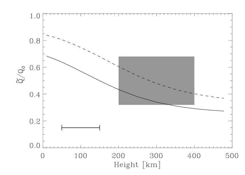
Figure 10: Hanle depolarization produced by the dynamo simulations. The depolarization of Sr i $\lambda$4607 Å is represented versus the height in the atmosphere where the depolarizing collisions are evaluated. The two types of line represent different scalings of the dimensionless magnetic field strength: the one used along the paper (the solid line), and a factor two smaller (the dashed line). The shaded region corresponds to measurements of the depolarization close to the solar disk center (see Faurobert-Scholl et al. 1995). The segment points out the range of heights that we ascribe to the dynamo simulation for the synthesis of Fe I 6302.5 Å.

In case that the magnetic field strength is not unique but has a distribution of values, the mean signal $\widetilde{Q}/Q_{0}$ turns out to be equal to the mean depolarization factor considering the distribution of the field strengths $\widetilde{W}_{B}$ (see Landi Degl’Innocenti 1985, §3). Note that $W_{B}$ no longer varies with $B$ as $B\gg B_{H}$ ($\gamma_{H}\gg 1$), therefore the average depolarization $\widetilde{W}_{B}$ bears no information on the large field strengths that may exist in the distribution. In other words, the mean signal will always be biased towards weak field strengths (e.g., Trujillo Bueno 2001, Fig. 3). This fact could reconcile the large fields in the dynamo simulations with the observed Hanle depolarization signals. In order to check such possibility, we evaluate the mean $\widetilde{W}_{B}$ for the snapshot studied in the paper. The transition and collision rates required to compute $B_{H}$ are determined, according to the prescription in Faurobert et al.(2001, §3), using the quiet Sun densities and temperatures given by Maltby et al. (1986). We only consider the photospheric layers. The expected signals, including all the magnetic fields in the snapshot describing the distribution of $B$, are represented in Figure 10. The depolarization changes with height due to the variation of temperature and density in the model atmosphere, which modify $B_{H}$. Figure 10 includes the range of Hanle signals observed close to the disk center, namely, $\widetilde{Q}/Q_{0}=0.50\pm 0.18$ (quoted by Faurobert-Scholl et al. 1995, from the measurements of Stenflo 1982 at an heliocentric angle whose cosine is $\mu=0.81$). The observational signal has been chosen to be as close as possible to the disk center to sample deep photospheric layers. The measurement of depolarization is ascribed by Faurobert-Scholl et al. (1995) to a range of heights between 200 km and 400 km. Although these layers are still too high for the range of heights that we assign to the simulation in the Zeeman syntheses (the base of the photosphere), the depolarization turns out to be within the bounds set by observations (see Fig. 10, the solid line). The agreement improves taking into account that the turbulent field strengths are expected to decrease with height in the atmosphere (e.g. Faurobert-Scholl et al. 1995). The dashed line in Figure 10 has been computed assuming the field strengths to be a factor of two smaller than those in the original snapshot. In short, our simplified estimate indicates no obvious inconsistency between the simulations and the observed Hanle effect depolarization signals for Sr I $\lambda$4607 Å.

6 What spatial resolution is necessary to resolve the numerical data?

Answering this question may be relevant to design of the next generation solar telescopes (Rosner & Beckers, 2001, private communication). For the sake of simplicity, we adopt the magnetic flux as the physical parameter to be determined. It is routinely measured using standard instrumentation, and it suffers a severe bias due to insufficient spatial resolution (§4.1). The fraction of magnetic flux in the simulation that one still detects in synthetic magnetograms is used to quantify the required angular resolution. This information is contained in Figure 3b, which we plot in a slightly different way in Figure 11. Abscissae and ordinates have been interchanged, and the angular resolution is also presented in terms of the diameter of the ideal telescope achieving the angular resolution (see equation [7]).This representation suits our present purposes. The curve is shown for two different sensitivities, i.e., when (virtually) all polarization signals are detected, and when only those larger than 20 G are above the noise level. The following conclusions follow from Figure 11:

1. Irrespective of the resolution, one only detects 80 % of the existing flux. The residual 20 % cancellation is due to the smearing along the line-of-sight produced by the radiative transfer. Surpassing this upper limit is not a question of increasing the telescope size but rather it demands improving the diagnostic techniques used to measure the magnetic flux.

2. Detecting 50 % of the flux would require an angular resolution of 110 km or a telescope of 85 cm. Detecting another 20 % additional magnetic flux demands resolving 40 km and so a telescope some three times larger (2.3 m).

3. Points #1 and #2 refer to observations without noise. If one considers a detection threshold of 20 G (which corresponds to a degree of polarization of some 0.3 %, according to the calibration in §3.2), then only 70 % of the flux present in the simulation can be detected. On the other hand detecting 50 % implies an angular resolution of 70 km or a diameter of $\simeq$ 1.3 m.

4. The slope of the solid line in Figure 11 drastically changes when trying to detect more than, say, 65 % of the original flux. Going beyond this point requires a large increase of telescope diameter for a limited increase of additional signal. This 65 % may represent an optimal compromise between resolution and telescope size, and it corresponds to 60 km on the Sun or a diameter of 1.5 m.

7 Discussion

The dynamo simulation by Cattaneo (1999) (see also Emonet & Cattaneo 2001) produce magnetic fields whose structure resembles in many ways the quiet Sun magnetic fields (§1). Although the simulations were not designed for a realistic description of the solar conditions, the quantitative comparison with the quiet Sun that we undertake is useful for a variety of reasons. It allows to judge whether, and to what extent, the turbulent dynamo provides a paradigm to describe the quiet Sun magnetism. It allows to identify, study and understand the difficulties and biases faced by the current observational techniques when applied to very complex fields. It helps identifying physical ingredients that are missing in the simulations, an exercise helpful to guide future numerical work. Finally, it may suggest the type of technical developments needed to measure the properties of a magnetic field with the complexity present in the numerical data. Keeping in mind all these reasons, we synthesize the polarization emerging from the simulation. Specifically, we choose a snapshot of the time series representative of the stationary regime, which renders some 2.6 $\times$ 10⁵ individual spectra. The assumptions and limitations of our Milne-Eddington approach to the synthesis are discussed in §3. They let us calculate the polarization produced by a magnetically sensitive spectral line similar to Fe I $\lambda$6302.5 Å. The synthetic spectra have been analyzed in the light of observations of quiet Sun magnetic fields. The comparison reveals similarities and differences. In addition, it provides some hints and caveats to keep in mind when interpreting observations. These three aspects of the synthetic spectra are discussed next.

The magnetograms produced by the numerical data are in good agreement with those observed in the Sun (§4.1, Figs. 3a and 4). The agreement, however is only achieved after a severe canceling of signals produced by the poor spatial resolution of the current observations. More than 90 % of the unsigned magnetic flux existing in the numerical data does not appear in magnetograms with 1″angular resolution (Fig. 3b). In other words, it is this 2 to 10 % residual that agrees with the observed signals. The Stokes $V$ profiles emerging from the simulation are frequently very asymmetric, in qualitative agreement with observations (see references in §1). In particular, Stokes $V$ profiles with three and more lobes result from the existence of two opposite polarities in the resolution element. Part of these asymmetries are produced by gradients of magnetic field and velocity along the line-of-sight (Fig. 5), but the Stokes $V$ profiles also owe much of their shapes to variations across the line-of-sight within the resolution element (cf. Figs. 5 and 6). We studied in §4.3 the excess of broadening of the synthetic intensity profiles due to the presence of a magnetic field. The additional broadening is found to be close to, but typically in excess of, the upper limit of 140 G set by Stenflo & Lindegren (1977). The uncertainties of the measurement could easily explain this discrepancy, therefore, we understand this marginal disagreement as an invitation to revisit the work by Stenflo & Lindegren (1977) and improve the sensitivity by a factor two. This should be enough clearly to confirm or discard a solar magnetic field with the features present in the numerical data. So far only Zeeman signals of typical photospheric lines have been mentioned. We also estimate in §5 the Hanle depolarization to be expected if the simulation is placed at various heights in the photosphere. All the uncertainties notwithstanding, the depolarization signals for Sr I $\lambda$4607 Å  turn out to be within the observed bounds.

A quantitative analysis of the Stokes $V$ asymmetries reveals real discrepancies between the synthetic spectra and the quiet Sun. Most of the synthetic profiles show mild asymmetries, well below the mean observed values. Moreover, the synthetic spectra do not contain the clear observed tendency for the Stokes $V$ blue lobe to dominate. Such trend is present even in the largest polarization signals, which trace big concentrations of magnetic field. We believe that the cause of the discrepancy is twofold. First, the dispersion of velocities between nearby pixels is too small. Second, the spatial separation between strongly magnetized and unmagnetized plasmas is too large. These two factors minimize the asymmetries in the intergranular lanes, despite the fact that the kind of correlation between magnetic field and velocity already existing in the simulation produces the right asymmetry. Arguments for such explanation are given in §4.2. As a support of this view, we artificially increase the dispersion of velocities and magnetic fields existing in the simulation to synthesize spectra in three particularly large magnetic concentrations. The resulting Stokes $V$ profiles look very much like those observed in the quiet Sun network (synthetic and observed profiles are represented in Fig. 8). If we have correctly identified the origin of the differences, what must be modified in the numerical simulation in order to produce asymmetries closer to the observed ones? One would need to increase the dispersion of velocities and magnetic fields at the smallest spatial scales, keeping the relationship between them already existing in the simulation. This could be attained by increasing the Reynolds numbers of the simulations.

There is another discrepancy between the synthetic and the observed profiles which has not been mentioned yet. The analysis of Stokes $V$ shapes observed in the quiet Sun reveals that kG field strengths are common (see Sánchez Almeida & Lites 2000, Socas-Navarro & Sánchez Almeida 2002). There are also weaker fields (e.g., Lin & Rimmele 1999; Collados 2001), but the frequency of kG is certainly larger than that present in the simulation. This difference can be readily pin down to the incompressibility of the simulation (§2), which hampers the strong evacuation of the plasma, an ingredient always associated with the existence of kG fields in the photosphere.

We have found several similarities between the synthetic spectra emerging from the dynamo simulation and observations of quiet Sun magnetic fields. Such (sometimes unexpected) agreement seems to point out that the simulation already capture some of the essential features characterizing the quiet Sun magnetic fields. These arguments enables us to proceed by analogy and propose the existence of magnetic fields on the Sun similar to those in the numerical simulations. Several interesting consequences follow from this assumption:

1. The amount of flux inferred by conventional magnetograms depends very much on the angular resolution and the sensitivity of the measurements. Good or very good sensitivity is mandatory to detect any fluxes with the canonical 1″angular resolution. For example, the structures in the numerical simulation would be very difficult to detect in magnetograms like those provided by the MDI instrument on board the SOHO spacecraft, with a sensitivity of some 15 G (e.g., Liu & Norton 2001). According to Figure 3b, only 1% of the original magnetic flux is detectable at this sensitivity level. On the other hand, the sensitivity is not so critical upon improvement of the angular resolution. In the limit of perfect angular resolution the signals become of the order of 50 G, corresponding to a degree of circular polarization of 1% (see Fig. 5).

2. The amount of unsigned flux existing in the simulation is also very large in absolute terms. Assuming that the full solar surface were covered by magnetic fields like those in the numerical simulations, the associated total unsigned flux would be of the order of $3.1~{}\times~{}10^{24}$ Mx. This figure is a factor 4.5 times larger than the total flux detected at solar maximum with conventional techniques (Rabin et al. 1991, Fig. 5). Should such large amounts of hidden flux exist in the photosphere, it would have to interact with the other classical manifestations of the solar magnetism (active regions, solar cycle, coronal heating, etc). This point in particular deserves further investigations.

3. We discuss in §6 the telescope size required to detect the magnetic structures observed in the simulations. This is a preliminary estimate which certainly has to be revised and refined. (For example, we do not address the question of whether the 60 km optimum spatial resolution is set by the photon mean-free-path or the diffusion processes included in the MHD simulation.) However one conclusion of this preliminary study stands out. A sizeable fraction of the magnetic flux is not detected due to the radiative transfer smearing along the line-of-sight. Improving such bias is not a matter of increasing the telescope size and polarimetric sensitivity. It only depends on interpreting the observed polarization using techniques that account for the line-of-sight smearing. Keeping in mind the complexity of the fields (e.g., the longitudinal magnetic field almost always changes sign along the line-of-sight; see Fig. 7c), the use of inversion techniques that assume optically thin fluctuations of the magnetic field seems to be a reliable selection (e.g., the MISMA inversion code in Sánchez Almeida 1997).

4. The Stokes asymmetries contain information on the magnetic structuring at spatial scales smaller than the resolution element, an information unique and valuable (see §1). The syntheses show that both variations along the line-of-sight and across the line-of-sight are responsible for the asymmetries. Consequently, the inversion techniques aimed at understanding the origin of the asymmetries, and therefore at measuring the properties of the photospheric magnetic fields, have to incorporate the two aspects of the spatial variations.

The importance of the above conclusions depends to some extent, on the degree of realism of the simulations. However, the tendencies that they imply are probably correct; e.g., the existence of large amounts of solar magnetic flux missing in conventional measurements, or the need for non-standard inversion techniques to determine the properties of the quiet Sun magnetic fields. These problems are important enough to deserve a close follow-up.

Figure 1: Approximation used to synthesize the polarized spectrum. The solid lines show Stokes $I$, $Q$, $U$ and $V$ profiles from a point of the simulation synthesized according to the MISMA approximation employed along the text. The dashed lines represent a full integration of the radiative transfer equations. Typical relative deviations are of the order of a few per cent. Wavelengths are in mÅ and the Stokes profiles have been normalized to the continuum intensity.

Figure 3: Mean flux density as a function of the spatial resolution of an hypothetical observation. The three different curves represent different sensitivities of the observation (0.5 G, the solid lines; 5 G, the dotted lines; 20 G, the dashed lines). (a) The flux density in the synthetic magnetogram is given in G. The symbols represent real observations of IN fields. For the equivalence between symbol and reference, see §4.1. (b) The flux density has been normalized to the true mean flux density, i.e., the mean value of $|B_{z}|$ in the simulation. It helps understanding the large fraction of missing flux for the sensitivity and angular resolution of a typical observation (say, 5 G and 1″). Note the 20 % reduction for perfect angular resolution, which is produced by the radiative transfer smearing along the line-of-sight. The arrow on the abscissae points out 1″.

Figure 5: Types of Stokes $V$ profiles produced by the numerical simulation. All plots share a common scale which is indicated at the bottom of the figure. The label of each profile includes a number for cross-reference, and the percentage of profiles in the simulation belonging to the category. The profiles have been taken from the original simulation, with no spatial smearing. The large plus sign of each plot indicates the origin of the horizontal and vertical scales, shown at the bottom of the figure. The Stokes $V$ profiles are normalized to the continuum intensity.

Figure 6: Same as Figure 5, except that the synthetic profiles have been smeared with a 1″ seeing. The variety of possibilities has increased.

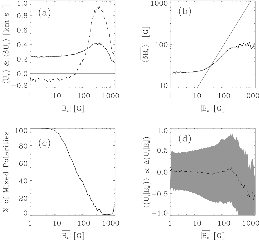
Figure 7: Variations along the line-of-sight of the longitudinal magnetic field and the longitudinal velocity. We represent mean values among all those points in the simulation having the line-of-sight mean longitudinal magnetic field given in the abscissae ($\overline{B_{z}}$; see equations [11] to [15] for definitions). (a) Mean vertical velocity (the dashed line) as well as the mean standard deviation among the velocity fluctuations along the line-of-sight (the solid line). ($U_{z}>0$ corresponds to downflows or redshifts.) (b) Mean standard deviation of the magnetic field fluctuations along the line-of-sight. The oblique straight line $y=x$ is included for reference. (c) Percentage of points where the longitudinal magnetic field changes sign along the line-of-sight. (d) Correlation coefficient for the fluctuations of magnetic field and velocity along the line-of-sight. The dashed line corresponds to the mean value, $\langle\overline{(U_{z}|B_{z}|)}\rangle$, whereas the shaded region shows one standard deviation about this mean value, $\langle\overline{(U_{z}|B_{z}|)}\rangle\pm\Delta\overline{(U_{z}|B_{z}|)}$. Velocities and magnetic fields are in km s^-1 and G, respectively. The correlation coefficients are dimensionless.

Figure 8: (a), (b), and (c) correspond to the synthetic Stokes $V$ profiles resulting form the average of the patches $a$, $b$ and $c$ in Figure 2. (d) Observed profile shown for reference. It is the class 3 profile in Figure 4 of Sánchez Almeida & Lites (2000).

Figure 9: Difference between the Stokes $I$ profiles synthesized with and without magnetic fields ($I-I_{\rm non-magnetic}$). The difference has been modeled as the difference of two Gaussian functions (the dashed line) whose different widths correspond to an apparent magnetic field of the order of 220 G. (See text for details.)

Figure 11: Spatial resolution required to detect a given fraction of the magnetic flux density present in the numerical simulation. The diameter of a diffraction limited telescope that yields the required spatial resolution is given in the second axis of ordinates. The solid line represents observations without noise whereas the dashed line corresponds to a noise of 20 G, equivalent to a degree of polarization of some 0.3% . Angular resolutions are in Mm and telescope diameters in m.

References

- Babcock (1953) Babcock, H. W. 1953, ApJ, 118, 387
- Baur et al. (1981) Baur, T. G., Elmore, D. E., Lee, R. H., Querfeld, C. W., & Rogers, S. R. 1981, Sol. Phys., 70, 395
- Beckers (1969) Beckers, J. M. 1969, Sol. Phys., 9, 372
- Bellot Rubio et al. (1997) Bellot Rubio, L. R., Ruiz Cobo, B., & Collados, M. 1997, ApJ, 478, L45
- Berger et al. (1998) Berger, T. E., Löfdahl, M. G., Shine, R. A., & Title, A. M. 1998, ApJ, 506, 439
- Berger & Title (1996) Berger, T. E., & Title, A. M. 1996, ApJ, 463, 365
- Berger & Title (2001) Berger, T. E., & Title, A. M. 2001, ApJ, 553, 449
- Bianda et al. (1999) Bianda, M., Stenflo, J. O., & Solanki, S. K. 1999, A&A, 350, 1060
- Bonet (1999) Bonet, J. A. 1999, in ASSL, Vol. 239, Motions in the Solar Atmosphere, ed. A. Hanslmeier & M. Messerotti (Dordrecht: Kluwer), 1
- Cattaneo (1999) Cattaneo, F. 1999, ApJ, 515, L39
- Cattaneo et al. (2001) Cattaneo, F., Lenz, D., & Weiss, N. . 2001, ApJ, 563, L91
- Collados (2001) Collados, M. 2001, in ASP Conf. Ser., Vol. 236, Advanced Solar Polarimetry – Theory, Observations, and Instrumentation, ed. M. Sigwarth (San Francisco: ASP), 255
- Domínguez Cerdeña et al. (2002) Domínguez Cerdeña, I., Kneer, F., & Sánchez Almeida, J. 2002, ApJ, submitted
- Durrant (1982) Durrant, C. J. 1982, in Landolt-Börnstein, Vol. 2a, Astronomy Astrophysics & Space Research, ed. K. Schaifers & H. H. Voigt (Berlin: Springer-Verlag), 96
- Elmore et al. (1992) Elmore, D. F., et al. 1992, Proc SPIE, 1746, 22
- Emonet & Cattaneo (2001) Emonet, T., & Cattaneo, F. 2001, ApJ, 560, L197
- Faurobert et al. (2001) Faurobert, M., Arnaud, J., Vigneau, J., & Frish, H. 2001, A&A, 378, 627
- Faurobert-Scholl et al. (1995) Faurobert-Scholl, M., Feautrier, N., Machefert, F., Petrovay, K., & Spielfiedel, A. 1995, A&A, 298, 289
- Grigorjev & Katz (1972) Grigorjev, V. M., & Katz, J. M. 1972, Sol. Phys., 22, 119
- Grossmann-Doerth et al. (1996) Grossmann-Doerth, U., Keller, C. U., & Schüssler, M. 1996, A&A, 315, 610
- Grossmann-Doerth et al. (1988) Grossmann-Doerth, U., Schüssler, M., & Solanki, S. K. 1988, A&A, 206, L37
- Grossmann-Doerth et al. (1989) Grossmann-Doerth, U., Schüssler, M., & Solanki, S. K. 1989, A&A, 221, 338
- Jefferies & Mickey (1991) Jefferies, J. T., & Mickey, D. L. 1991, ApJ, 372, 694
- Keller et al. (1994) Keller, C. U., Deubner, F.-L., Egger, U., Fleck, B., & Povel, H. P. 1994, A&A, 286, 626
- Landi Degl’Innocenti (1976) Landi Degl’Innocenti, E. 1976, A&AS, 25, 379
- Landi Degl’Innocenti (1985) Landi Degl’Innocenti, E. 1985, Sol. Phys., 102, 1
- Landi Degl’Innocenti (1992) Landi Degl’Innocenti, E. 1992, in Solar Observations: Techniques and Interpretation, ed. F. Sánchez, M. Collados, & M. Vázquez (Cambridge: Cambridge University Press), 71
- Landi Degl’Innocenti & Landi Degl’Innocenti (1973) Landi Degl’Innocenti, E., & Landi Degl’Innocenti, M. 1973, Sol. Phys., 31, 299
- Landi Degl’Innocenti & Landolfi (1983) Landi Degl’Innocenti, E., & Landolfi, M. 1983, Sol. Phys., 87, 221
- Lin & Rimmele (1999) Lin, H., & Rimmele, T. 1999, ApJ, 514, 448
- Lites et al. (1994) Lites, B. W., Martínez Pillet, V., & Skumanich, A. 1994, Sol. Phys., 155, 1
- Liu & Norton (2001) Liu, Y., & Norton, A. A. 2001, Mdi measurement errors: the magnetic perspective, Technical Report SOI O1-144, Center for Space Science and Astrophysics, Stanford University
- Makita (1986) Makita, M. 1986, Sol. Phys., 106, 269
- Maltby et al. (1986) Maltby, P., Avrett, E. H., Carlsson, M., Kjeldseth-Moe, O., Kurucz, R. L., & Loeser, R. 1986, ApJ, 306, 284
- Meneguzzi & Pouquet (1989) Meneguzzi, M., & Pouquet, A. 1989, J. Fluid Mech., 205, 297
- Moore et al. (1966) Moore, C. E., Minnaert, M. G. J., & Houtgast, J. 1966, The Solar Spectrum from 2935 Å to 8770 Å , NBS Mono. 61 (Washington: NBS)
- Petrovay & Szakaly (1993) Petrovay, K., & Szakaly, G. 1993, A&A, 274, 543
- Rabin et al. (1991) Rabin, D. M., Devore, C. R., Sheeley, N. R., Harvey, K. L., & Hoeksema, J. T. 1991, Solar interior and atmosphere, ed. A. N. Cox, W. C. Livingston, & M. S. Matthews (The University of Arizona Press), 781
- Roddier (1981) Roddier, F. 1981, in Progress in Optics, ed. E. Wolf, Vol. 19 (Amsterdam: North-Holland Publishing Co.), 281
- Sánchez Almeida (1997) Sánchez Almeida, J. 1997, ApJ, 491, 993
- Sánchez Almeida (1998) Sánchez Almeida, J. 1998, ApJ, 497, 967
- Sánchez Almeida et al. (1988) Sánchez Almeida, J., Collados, M., & del Toro Iniesta, J. C. 1988, A&A, 201, L37
- Sánchez Almeida et al. (1989) Sánchez Almeida, J., Collados, M., & del Toro Iniesta, J. C. 1989, A&A, 222, 311
- Sánchez Almeida et al. (1996) Sánchez Almeida, J., Landi Degl’Innocenti, E., Martínez Pillet, V., & Lites, B. W. 1996, ApJ, 466, 537
- Sánchez Almeida & Lites (1992) Sánchez Almeida, J., & Lites, B. W. 1992, ApJ, 398, 359
- Sánchez Almeida & Lites (2000) Sánchez Almeida, J., & Lites, B. W. 2000, ApJ, 532, 1215
- Schüssler (1986) Schüssler, M. 1986, in Small Scale Magnetic Flux Concentrations in the Solar Photosphere, ed. W. Deinzer, M. Knölker, & H. H. Voigt (Göttingen: Vandenhoeck & Ruprecht), 103
- Sigwarth (2001) Sigwarth, M. 2001, ApJ, 563, 1031
- Sigwarth et al. (1999) Sigwarth, M., Balasubramaniam, K. S., Knölker, M., & Schmidt, W. 1999, A&A, 349, 941
- Skumanich & Lites (1987) Skumanich, A., & Lites, B. W. 1987, ApJ, 322, 473
- Socas-Navarro (2001) Socas-Navarro, H. 2001, in ASP Conf. Ser., Vol. 236, Advanced Solar Polarimetry – Theory, Observations, and Instrumentation, ed. M. Sigwarth (San Francisco: ASP), 487
- Socas-Navarro & Sánchez Almeida (2002) Socas-Navarro, H., & Sánchez Almeida, J. 2002, ApJ, 565, 1323
- Solanki & Montavon (1993) Solanki, S. K., & Montavon, C. A. P. 1993, A&A, 275, 283
- Solanki & Pahlke (1988) Solanki, S. K., & Pahlke, K. D. 1988, A&A, 201, 143
- Spiegel & Veronis (1960) Spiegel, E. A., & Veronis, G. 1960, ApJ, 131, 442
- Steiner (2000) Steiner, O. 2000, Sol. Phys., 196, 245
- Stenflo (1982) Stenflo, J. O. 1982, Sol. Phys., 80, 209
- Stenflo (1994) Stenflo, J. O. 1994, Solar Magnetic Fields, ASSL 189 (Dordrecht: Kluwer)
- Stenflo et al. (1984) Stenflo, J. O., Harvey, J. W., Brault, J. W., & Solanki, S. K. 1984, A&A, 131, 333
- Stenflo & Lindegren (1977) Stenflo, J. O., & Lindegren, L. 1977, A&A, 59, 367
- Stolpe & Kneer (2000) Stolpe, F., & Kneer, F. 2000, A&A, 353, 1094
- Topka & Title (1991) Topka, K. P., & Title, A. M. 1991, Solar interior and atmosphere, ed. A. N. Cox, W. C. Livingston, & M. S. Matthews (The University of Arizona Press), 727
- Trujillo Bueno (2001) Trujillo Bueno, J. 2001, in ASP Conf. Ser., Vol. 236, Advanced Solar Polarimetry – Theory, Observation, and Instrumentation, ed. M. Sigwarth (San Francisco: ASP), 161
- Trujillo Bueno & Manso Sainz (1999) Trujillo Bueno, J., & Manso Sainz, R. 1999, ApJ, 516, 436
- Unno (1956) Unno, W. 1956, PASJ, 8, 108
- Unno (1959) Unno, W. 1959, ApJ, 129, 375
- Wang et al. (1995) Wang, J., Wang, H., Tang, F., Lee, J. W., & Zirin, H. 1995, Sol. Phys., 160, 277
- Wittmann (1974) Wittmann, A. 1974, Sol. Phys., 35, 11
- Yi & Engvold (1993) Yi, Z., & Engvold, O. 1993, Sol. Phys., 144, 1