Abstract

X-ray emission features have been detected in at least five GRB afterglows. Their detection and properties are of great importance in our understanding of the nature of the GRB progenitor. Moreover, they provide us with an un-collimated source of photons, allowing us to put firm constraints on the total energy produced in GRBs, and therefore on their degree of collimation. I will review the radiation mechanisms and geometries proposed as sources of the line emission, and discuss the energy budget of the lines and their implication for the overall energetics of the phenomenon.

1 Introduction

The detection of X-ray emission lines in the afterglow of Gamma-Ray Bursts (GRBs) allows us to probe the close GRB environment and therefore gives clues on the nature of the progenitor. Moreover, being un-collimated, line emission can be used to constrain the energy budget of the bursts and therefore their beaming angle.

There are at least five GRBs to date with evidence for X-ray emission features in their early X-ray afterglow. Two of them were detected by BeppoSAX (GRB 970508 [1] and GRB 000214 [2]), one by ASCA (GRB 970828 [3]), one by Chandra (GRB 991216 [4]) and one by XMM-Newton (GRB 011211 [5]). Even though none of these features has a strictly compelling evidence (all are less than $5\sigma$ statistical confidence), their number, the coincidence with expected emission lines (in all the cases in which an alternative redshift is known) and the fact that the features have been detected by all the X-ray missions capable of doing so, make the presence of these features difficult to challenge. The properties of the detected lines are summarized in Table 1. Additional evidence for the presence of lines or line complexes were also suggested for two more XMM-Newton spectra of GRB 001025A and GRB 010220 [6] and the detection of a transient absorption feature in the X-ray prompt emission of GRB 990705 [7]. Finally it should be mentioned that there are cases in which, despite prompt and deep searches, the presence of emission features could be excluded at flux levels and equivalent widths (EW) much fainter than the detected ones (e.g. in GRB 020405 [8]).

GRB 970508 970828 991216 000214 $z_{\rm{opt}}$ 0.835 0.958^∗ 1.02 0.46^∗ Line ID Fe Fe Fe Fe $F_{\rm{line}}^{[a]}$ $30\pm 10$ $15\pm 8$ $17\pm 5$ $6.7\pm 2.2$ $h\nu$ (keV) $3.4\pm 0.3$ $5\pm 0.25$ $3.5\pm 0.06$ $4.7\pm 0.2$ EW(keV) 1.5 3 0.5 2 $t_{s}-t_{e}^{\ddagger}$ 6–16 32–38 37–40 12–41 $L^{\rm{iso}}_{44}$ (erg/s) $12\pm 4$ $8.1\pm 4.3$ $11\pm 3$ $0.6\pm 0.2$ $E^{\rm{iso}}_{49}$ (erg) $3.6\pm 1.3$ $5\pm 3$ $7.7\pm 2.3$ $0.6\pm 0.3$ Ref. [1] [3] [4] [2] $\theta_{j}^{[b]}$ 16.7 4.1 2.9 $E_{\gamma,51}^{\rm{F01}[c]}$ 0.23 0.57 0.69 $E_{\gamma,51}^{[d]}$ 11–18 4.5–25 3–38 2–3

GRB 011211 011211 011211 011211 $z_{\rm{opt}}$ 2.14 2.14 2.14 2.14 Line ID Si S Ar Tot^† $F_{\rm{line}}^{[a]}$ $1.1\pm 0.3$ $1.\pm 0.3$ $0.7\pm 0.3$ $4\pm 1.6$ $h\nu$ (keV) $0.71\pm 0.02$ $0.88\pm 0.01$ $1.21\pm 0.02$ - EW (keV) 0.43 0.48 0.46 $t_{s}-t_{e}^{\ddagger}$ 11-12.4 11-12.4 11-12.4 11-12.4 $L^{\rm{iso}}_{44}$ (erg/s) $4.3\pm 1.2$ $3.9\pm 1.1$ $2.6\pm 1$ $15.6\pm 6.3$ $E^{\rm{iso}}_{49}$ (erg) $0.6\pm 0.2$ $0.55\pm 0.16$ $0.4\pm 0.14$ $2.2\pm 0.9$ Ref. [5] [5] [5] [5] $E_{\gamma,51}^{[d]}$ 0.5–4.4

Table 1: Properties of the lines detected so far in the early afterglows of GRBs.   ^∗: these bursts do not have an optical determination of the redshift, which is inferred from the X-ray line, identified as a FeXXVI $K_{\alpha}$ line.   ^† In this column all the five lines detected by Reeves et al. [5] are added together.   ^‡ the start and end times of the observations, or the time at which the line is observed to disappear.   ^[a]: units of erg cm^-2 s^-1.   ^[b]: the opening angle of the jet in degrees as measured from the afterglow break time [28].   ^[c]: total energy in $\gamma$-rays in units of $10^{51}$ erg as measured by correcting the GRB fluence for the solid angle [28].   ^[d]: total energy in $\gamma$-rays in units of $10^{51}$ erg as measured from the emission lines fluence [27].

2 Line properties

In this section I will summarize the “average” properties of the detected features. I will in particular emphasize what are the characteristics of the lines which are most difficult to explain in the simplest GRB scenario. The measured properties of the individual emission features are reported in Tab. 1.

Luminosity

The luminosity of the detected lines are large, and reproducing the observed luminosities of these features is one of the big challenges of theoretical models.

$$L\sim\mathrm{few}\times 10^{44}\quad\mathrm{erg~{}s}^{-1}$$ (1)

Equivalent width

In addition to the large measured luminosities, the contrast of the emission features with respect to the continuum is large. Again, this is a challenging property for the models.

$$EW\sim 1\quad\mathrm{keV}$$ (2)

Frequency

The observed frequency of the line emission is, in all cases for which an optical redshift is known, consistent with emission from iron (either neutral or highly ionized). In one case (GRB 011211 [5]) several lighter element lines were detected. A proper velocity of the emitting material has been inferred in all the “good quality” detections [4, 5].

Duration

The duration of the line emission is not completely clear, due to the limitation of the performed observations. Most of the lines have been observed to be active at comoving times

$$T\sim 10\quad\mathrm{h}$$ (3)

Some lines are observed to disappear during the observations [1, 3, 5], some are observed to remain constant while the continuum fades [2] while in some cases the observations were too short to allow for any conclusion [4].

3 First Consequences

In this section I will review the first consequences that stem from the mere detection of these lines with the fiducial properties reported in the above section.

Reprocessing

The lines are detected at a frequency consistent with the expected emission lines from heavy elements in the rest frame of the host galaxy of the bursts. At the time of detection, the fireball is expected to be still highly relativistic [9] ($\Gamma>10$). Therefore, the fact that no blueshift (or only moderate [5]) is observed implies that the line photons are not produced directly within the fireball itself, but by material at rest in the host galaxy

Large densities

It is easy to show that, given the observed properties of the lines, a large density of the producing (or reprocessing) material is required [9]. Let us assume, in fact, that the lines are produced in a low density medium, so that no recombination takes place. Let us also consider iron lines (analogous conclusions can be obtained for different elements). Given the line luminosity and duration of the emission, we can compute the total number of line photons emitted:

$$N_{\mathrm{Fe}}={{L_{\mathrm{line}}\,t_{\mathrm{line}}}\over{h\nu_{\mathrm{line}}}}\sim 10^{57}$$ (4)

where we used the luminosity and duration given in Eq. 1 and 3. Since each iron atom can produce at most 10 line photons [11] (given the effects of Auger auto-ionization) the total mass of reprocessing iron can be computed and, assuming a solar metallicity, the total mass of the reprocessing medium involved in the line emission:

$$M={{N_{\mathrm{Fe}}}\over{10}}{{m_{p}}\over{4.67\times 10^{-5}}}\sim 2000\,M_{\odot}$$ (5)

The size of the emitting region can be constrained by considering that the light travel time cannot be too long, otherwise the total energy carried by line photons would be larger than the burst energy. This yields a limit

$$R\leq c\,t_{\mathrm{line}}\leq 3\times 10^{17}\quad\mathrm{cm}$$ (6)

where we have allowed for a rather long duration of the line $t_{\mathrm{line}}\sim 100$ days. The lower limit on the density can be now computed by simply dividing the mass over the volume occupied by the medium:

$$n\geq{{M}\over{m_{p}\,V}}\sim{{N_{\mathrm{Fe}}}\over{10}}{{1}\over{4.67\times 10^{-5}}}{{3}\over{4\pi\,R^{3}}}\sim 2\times 10^{7}\quad\mathrm{cm}^{-3}$$ (7)

Analogous limits are obtained if, instead of assuming no recombination, we ask a density large enough to allow for efficient recombination of free electrons onto iron ions in the time scale of the GRB duration.

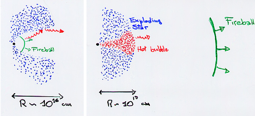
Figure 1: Cartoons showing the basic features of the two classes of models described in the text. The left panel shows the “Geometry Dominated” (GD) models, while the right panel shows the “Engine Dominated” (ED) models.

4 The two classes of models

The constraint on the density derived above poses a serious problem to the overall modelling of the events. Consider, as an example, the case of GRB 991216.Its afterglow lasted one month [12]. A fireball expanding in a high density medium should show a non-relativistic transition which was not observed in the data. Moreover, all the multiwavelength afterglow lightcurves can be modeled with low density environments [13]. Solving this apparent riddle of requiring a very high density to produce the lines and a very low one to account for the power-law afterglows is the most formidable tasks of all the theories willing to explain how the lines have been formed.

The solutions that have been put forward to date can be divided in two classes: those requiring a strong anisotropy of the surrounding medium (a low density line of sight surrounded by high density material) and those calling for a very small and dense reprocessor, which lies inside the fireball and is surrounded by a low density ambient (see Fig. 1). In these two classes of models, an important difference is the reason for the observed duration of the line emission.

4.1 Geometry Dominated Models

For historical reasons I will discuss first the class of Geometry Dominated (GD) models, first discussed by Lazzati et al. in 1999 [9]. The basic idea of these class of models is that the line emission comes from an extended region surrounding the GRB progenitor. While the line emission takes place in a short period of time (maybe the $\sim 100$ seconds of the burst duration only) the observer at infinity receives line photons for a longer time, set by the light crossing time of the emitting region. The typical size of the emitting region is of the order of $R\sim 10^{16}$ cm. Since the region is large, the energy input is taken from the GRB and early afterglow continuum, which is reprocessed through reflection off a cold slab into line photons [14, 15].

The origin of the reprocessing material, which is likely to be moderately enriched in heavy elements, is thought to be the remnant of a recently exploded supernova [16] (SN) or a relic disk due to the interaction of the burst progenitor with a companion star [17]. The shape of this remnant was initially supposed to be a partial covering shell, but the detection of outward velocities of the reprocessing material made it more likely to think of a funnel-like structure [18] (see the left panel of Fig. 1). Such an extreme geometry may be due to the hyper-Eddington emission phase of the burst progenitor between the SN and the burst proper explosions.

Even though the line emission mechanism is supposed to be the reflection of the incident continuum off the cold dense material of the funnel walls, a possible alternative is represented by an optically thin shell of plasma, heated to $T\sim 10^{8}$ K by the burst photons themselves [5, 19]. Such an alternative, however, would require an extremely clumped shell [15], and would be quite difficult to explain the lack of detection of an iron (or cobalt or nickel) line in the afterglow of GRB 011211 [5].

The existence of dense material in the surroundings of at least some GRBs is corroborated by the detection of a transient absorption feature in the afterglow of GRB 990705 [7]. Such a feature can be accounted for by the presence of a fraction of a solar mass of iron at a distance $R\sim 2\times 10^{16}$ cm from the burst [11].

4.2 Engine Dominated Models

The class of GD models, even though provide us with a self-consistent scenario for the production of the detected lines, requires a two step explosion (first the SN and then the burst) and a rather extreme geometrical setup. More recently, alternative models have been presented. In this class of Engine Dominated models (ED), the line reprocessing material is supposed to be contained in a very small region, which is left behind by the fireball which therefore expands in a low density medium, as required by the afterglow observations and modelling (right panel of Fig. 1). The origin of this dense material is the progenitor star itself [20, 21].

The open problem for ED models is to find a suitable source of energy in order to power the line emission, since the fireball has already escaped and cannot contribute to the line production. Two possibilities have been discussed. In the first case, the energy may be provided by the inner engine itself, which instead of turning off abruptly at the end of the GRB emission remains active at a lower level for a longer time, powering the line emission through reflection off the surface of the funnel through which the fireball crossed the star [20]. Alternatively, the energy may be stored in the cocoon that surrounds the jet as it crosses the star [21]. In this case, however, it is difficult to have a mixing of the jet and mantle material tuned to make the bubble hot enough to power the line but not to explode as a second slower fireball.

An additional problem of the ED models is the nickel decay time. In usual SN explosions, in fact, iron is directly synthesized in very small quantities, while unstable nickel is produced in large quantities (up to a fraction of a solar mass). The unstable ⁵⁶Ni decays into ⁵⁶Co in a time scale of $\sim 6$ days which decays into ⁵⁶Fe after $\sim 80$ days. In conclusion, in a typical young supernova remnant, iron is the dominant element (over Ni and Co) starting from $\sim 100$ days after the explosion. For this reason, in ED models, nickel emission lines should be observed rather then iron ones. This problem can be ameliorated by downscattering [22] or by invoking a high neutronization during the SN explosion, which would lead to the direct synthesis of iron. In this latter case, however, no contribution from the SN should be observed in the afterglow, contrary to recent observations [23].

4.3 The spectrum of GRB 011211

The spectral features detected in the spectrum of GRB 011211 may represent a cornerstone in our understanding of the line production mechanism. In fact, the detection of large EW $K_{\alpha}$ lines from elements such as Mg, Si, S, Ar and Ca [5], can be explained, within the framework of reflection models, only if the continuum radiation that illuminates the reflecting material is hidden to the observer [15]. In fact, if a reflected spectrum is added to the incident one, the EW of S lines cannot be larger than $\sim 100$ eV, while Reeves et al. [5] detected a S line with $EW=480\pm 140$ eV, which can be explained only if the emitted line is not diluted into the incident continuum radiation.

Such a condition can be achieved in a contrived geometry or, more simply, can be due to light travel effects, if the reflecting material lies at a certain distance from the burst explosion site away from the line of sight [9]. The observer at infinity will in fact receive the undeflected ionizing continuum at a time $t_{0}$ and the reflected component at a time $t_{0}+R/c(1-\cos\theta)\gg{t}_{0}$ where $\theta$ is the angle between the line of sight and the line connecting the burst explosion site to the reflecting material.

The spectrum of GRB 011211 strongly suggests, therefore, that lines are produced in a GD scenario. It should be mentioned, however, that the line detection, albeit confirmed by the authors [24], has been challenged on data analysis [25] and on statistical [26] grounds, and all the conclusion above are therefore subject to revision, should the detection be proved false.

5 Line and burst energetics

Besides being a powerful probe of the condition of the close environment of GRBs, emission lines provide us with an isotropic emission that can be used to constrain the total energetics of the event [27]. The total energy of the burst as derived from the line emission can be written as:

$$E=E_{\mathrm{line,~{}iso}}\quad\epsilon_{\mathrm{line}}^{-1}\quad\epsilon_{\mathrm{spex}}^{-1}\quad\epsilon_{\mathrm{eff}}^{-1}$$ (8)

where $E_{\mathrm{line,~{}iso}}$ is the isotropic equivalent energy observed in line photons and $\epsilon_{\mathrm{line}}^{-1}$ is the efficiency of line production, i.e. the ratio of the line to incident continuum luminosity. $\epsilon_{\mathrm{spex}}^{-1}$ is the fraction of the burst spectrum in the X-ray band and $\epsilon_{\mathrm{eff}}^{-1}$ is the ratio of total energy to the energy in photons.

5.1 Line energetics

In order to obtain a measure of the total energy from Eq. 8 one has to estimate the total energy that is observed in the form of line photons. Besides the uncertainty on the line flux itself, the main problem is to evaluate the duration of the line emission. In fact, the observations start usually some time after the GRB, so that it is not possible to know the line flux at very early times. In addition, in several cases it is not possible to set a time for its turn-off time. In Tab. 1 we report the line energetics assuming that the line had a constant flux from the time of the GRB explosion up to the longer time in which it was detected, either the last observation or the moment in which it was observed to fade. See Ghisellini et al. [27] for a more complete discussion.

5.2 Line efficiency

In this section we evaluate the efficiency in the production of line photons by the reflection mechanism. Even though an accurate result can be obtained only with a numerical treatment [15, 27], we discuss here an approximate treatment that gives correct estimates. We concentrate here on iron lines, referring the reader to the literature for a more complete description [27].

The line emission efficiency can be estimated as the ratio of the energy in the photons absorbed by iron atoms in the layer of material with $\tau_{\mathrm{Fe}}=1$ to the total energy continuum photons, corrected for the fact that the energy of the line photon is lower than that of the photoionizing one. This yields:

$$\epsilon_{\mathrm{line}}\sim{{h\nu_{\mathrm{line}}\int_{\nu_{\mathrm{ph}}}^{\nu_{M}}{{{L(\nu)}\over{h\nu}}\left({{\nu}\over{\nu_{\mathrm{ph}}}}\right)^{-3}\,d\nu}}\over{\int_{\nu_{m}}^{\nu_{M}}L(\nu)\,d\nu}}$$ (9)

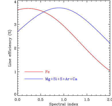
Figure 2: Line production efficiency in reflection models for iron (red line) and lighter elements as a function of the spectral index of the ionizing continuum. The lines show the result of the approximate Eq. 9.

Figure 3: Line production efficiency in reflection models for iron from the numerical computations of Lazzati et al. [15]. The efficiency is plotted against the ionization parameter, while different lines are relevant to different spectral indices and metallicities (see the above reference for more details).

The integral of Eq. 9 can be solved analytically for a power-law input spectrum, yielding the efficiency plotted in Fig. 3 as a function of the power-law index $\alpha$ [$L(\nu)\propto\nu^{-\alpha}$]. The approximation gives the maximum allowed efficiency, since it neglects the effect of the ionization parameter and of Auger autoionization. A numerical treatment [15] returns nevertheless consistent results within a factor of two (Fig 3), showing that this parameter is safely constrained to few per cent.

5.3 Bolometric correction

The bolometric correction to transform the X-ray energy into total radiative energy can be computed by assuming a Band spectrum with average values of the parameters (the two spectral slopes and the peak energy). This yields $\epsilon_{\mathrm{spex}}\approx 0.03\div 0.1$.

5.4 Radiative efficiency

The ratio of the energy in radiation to the total energy is the most uncertain and cannot be constrained. It should be remarked, however, that in order to compare the total energy inferred from line emission to the one estimated by Frail et al. [28], this correction is not necessary.

6 The total energy from lines

Before discussing how the total energy derived from line emission compares to other measurements it is worth discussing what we mean by the energetics of the GRB phenomenon. There are in fact at least three possible definitions of the total energy of the bursts.

The first possible definition is the real total energy involved in the explosion. This includes the energy that is released in gravitational waves, neutrinos, the possibly associated SN explosion and the burst itself. It may be of the order of $\sim 10^{54}$ erg in most of the progenitor models. Then, it is possible to define a usable energy for the GRB, which includes all the forms of energy that are more strictly related to the GRB phenomenology and/or can contribute emission during the burst and afterglow phases of the GRB explosion. This energy includes all the fireball energy, any precursor activity in photons or kinetic energy, any delayed output from the inner engine and energy stored in the jet cocoon (as discussed above). Is is clearly smaller than the real total energy involved in the explosion. Finally, what is more easy to measure is the fireball energy, and in particular the energy released in photons by the fireball. This is quite easy to constrain since we can measure the burst fluence and we have some tools to correct this energy input for any non-isotropy of the emission. This energy is clearly the smallest of the three.

Now, if we compute the total energy from Eq. 8, applying the fiducial values discussed above for the efficiencies involved, we obtain a rather large number (the data of GRB 991216 have been used as an example case):

$$E=3\times 10^{52}\,\left({{0.03}\over{\epsilon_{\mathrm{line}}}}\right)\,\left({{0.03}\over{\epsilon_{\mathrm{spex}}}}\right)\,\epsilon_{\mathrm{eff}}^{-1}\quad\mathrm{erg}$$ (10)

to be compared with the value of $E\sim 5\times 10^{50}$ measured by correcting the $\gamma$-ray isotropic energy times the solid angle of the jet, as derived from afterglow observations [28, 13].

The discrepancy is quite significant and calls for an explanation. There are two possible answers. First, the determination of the opening angle of the jet from the break time is prone to systematic uncertainties, related to the density of the ISM and to a possible missing constant into the equations (see e.g. the different approach of Rhoads [29] and Halpern et al. [30]). It is therefore possible that a systematic underestimate of the ISM density caused an underestimate of the opening angles and therefore of the total energy. Since, however, the ISM density comes into the equations with a very small power, this correction may ameliorate the discrepancy but it is unlikely to solve it completely.

Alternatively, it may be possible that the energy inferred from line emission is related to the usable energy for the GRB defined above rather than to the fireball energy. In this case, since the three energies discussed above define a nested sequence, there would not be any problem. However, if the fireball energy is indeed a very small fraction of the usable energy for the GRB, which is a very small fraction of the real total energy involved in the explosion, it is rather surprising that the fireball energy seems to be a remarkably well defined quantity [28, 13].

I am grateful to Martin Rees, Gabriele Ghisellini, Elena Rossi and Enrico Ramirez-Ruiz for the collaboration, the discussions and all the work done together.

Discussion

S. Kulkarni:  I am concerned that your adopted efficiency to convert the X-ray flux to line production is optimistic. Specifically, for 011211, with a narrow jet opening combined with high Lorentz factor would result in a photon beam which is quite narrow, a few degrees across. Does this not mean that you have to arrange your reflection surface in a very contrived way?

D. Lazzati:  What I am saying is that the lines require a total energy larger than what we obtain if we correct the $gamma$-ray observations for the beaming angles reported in the literature. If we relax this requirement, we can envisage a geometry in which a sizable fraction of the X-ray continuum is reprocessed. For example the walls of the reflecting funnel can be concave, or the reprocessing material may be in the form of clumps or filaments in a smaller version of the Crab remnant.

References

- [1] Piro L., Costa E., Feroci M., et al., ApJ, 514, L73 (1999).
- [2] Antonelli L. A., Piro L., Vietri M., et al., ApJ, 545, L39 (2000).
- [3] Yoshida A., Namiki M., Yonetoku D., et al., ApJ, 557, L27 (2001).
- [4] Piro L., Garmire G., Garcia M., et al., Science, 290, 955 (2000).
- [5] Reeves J. N., Watson D., Osborne J. P., et al., Nature, 416, 512 (2002).
- [6] Watson D., Reeves J. N., Osborne J., O’Brien P. T., Pounds K. A., Tedds J. A., Santos-Lleó M., Ehle M., A&A, 393, L1 (2002).
- [7] Amati L., Frontera F., Vietri M., et al., Science, 290, 953 (2000).
- [8] Mirabal N., Paerels F., Halpern J. P., ApJ submitted (astro-ph/0209516) (2002).
- [9] Lazzati D., Campana S., Ghisellini G., MNRAS, 304, L31 (1999).
- [10] Dado S., Dar A., De Rujula A., ApJ submitted (astro-ph/0207015) (2002).
- [11] Lazzati D., Ghisellini G., Amati L., Frontera F., Vietri M., Stella L., ApJ, 556, 471 (2001).
- [12] Halpern J. P., Uglesich R., Mirabal N., et al. ApJ, 543, 697 (2000).
- [13] Panaitescu A., Kumar P., ApJ, 571, 779 (2002).
- [14] Ballantyne D. R., Ramirez-Ruiz E., Lazzati D., Piro L., A&A, 389, L74 (2002).
- [15] Lazzati D., Ramirez-Ruiz E., Rees M. J., ApJ, 572, L57 (2002).
- [16] Vietri M., Stella L., ApJ, 507, L45 (1998).
- [17] Böttcher M., ApJ, 539, 102 (2000)
- [18] Vietri M., Ghisellini G., Lazzati D., Fiore F., Stella L., ApJ, 550, L43 (2001).
- [19] Lazzati D., A&A submitted (astro-ph/0210301) (2002).
- [20] Rees M. J., Mészáros P., ApJ, 545, L73 (2000).
- [21] Mészáros P., Rees M. J., ApJ, 556, L37 (2001).
- [22] McLaughlin G. C., Wijers R. A. M. J., Brown G. E., Bethe H. A., ApJ, 567, 454 (2002).
- [23] Bloom J. S., Kulkarni S. R., Price P. A., et al., ApJ, 572, L45 (2002).
- [24] Reeves J. N., Watson D., Osborne J. P., et al., A&A submitted (astro-ph/0206480) (2002).
- [25] Borozdin K., Trudolyubov S. P., ApJ submitted (astro-ph/0205208) (2002).
- [26] Rutledge R. E., Sako M., MNRAS in press (astro-ph/0206073) (2002).
- [27] Ghisellini G., Lazzati D., Rossi E., Rees M. J., A&A, 389, L33 (2002).
- [28] Frail D. A., Kulkarni S. R., Sari R., et al., ApJ, 562, L55 (2001).
- [29] Rhoads J. E., ApJ, 525, 737 (1999).
- [30] Sari R., Piran T., Halpern J. P., ApJ, 519, L17 (1999).