The superfluid two-stream instability and pulsar glitches

Abstract

This paper provides the first study of a new dynamical instability in superfluids. This instability is similar to the two-stream instability known to operate in plasmas. It is analogous to the Kelvin-Helmholtz instability, but has the distinguishing feature that the two fluids are interpenetrating. The instability sets in once the relative flow between the two components of the system reaches a critical level. Our analysis is based on the two-fluid equations that have been used to model the dynamics of the outer core of a neutron star, where superfluid neutrons are expected to coexist with superconducting protons and relativistic electrons. These equations are analogous to the standard Landau model for superfluid Helium. We study this instability for two different model problems. First we analyze a local dispersion relation for waves in a system where one fluid is at rest while the other flows at a constant rate. This provides a proof of principle of the existence of the two-stream instability for superfluids. Our second model problem concerns two rotating fluids confined within an infinitesimally thin spherical shell. The aim of this model is to assess whether the two-stream instability may be relevant (perhaps as a trigger mechanism) for pulsar glitches. Our results for this problem show that the entrainment effect could provide a sufficiently strong coupling for the instability to set in at a relative flow small enough to be astrophysically plausible.

1 Introduction

In this paper we describe a new dynamical instability in superfluids. This “two-stream” instability is analogous to the Kelvin-Helmholtz instability (Drazin & Reid, 1981). Its key distinguishing feature is that the two fluids are interpenetrating rather than in contact across an interface as in the standard scenario. The two-stream instability is well known in plasma physics [where it is sometimes referred to as the “Farley-Buneman” instability (Farley, 1963; Buneman, 1963, 1959)], and it has also been discussed in various astrophysical contexts like merging galaxies (Lovelace et al, 1997) and pulsar magnetopheres (Cheng & Ruderman, 1977; Weatherall, 1994; Lyubarsky, 2002), but as far as we are aware it has not been previously considered for superfluids. In fact, the “standard” Kelvin-Helmholtz instability was only recently discussed in the context of superfluids (Blaauwgeers et al, 2001).

The similarity of the equations used in plasma physics [a nice pedagogical description of the plasma two-stream instability can be found in Anderson et al (2001)] to the ones for two-fluid superfluid models inspired us to ask whether an analogous instability could be relevant for superfluids. That this ought to be the case seemed inevitable. To prove the veracity of this expectation, we have adapted the arguments from the plasma problem to the superfluid case, and discuss various aspects of the two-stream instability in this paper.

Of particular interest to us is the possibility that the two-stream instability may operate in rotating superfluid neutron stars. Mature neutron stars are expected to be sufficiently cold (eg. below $10^{9}$ K) that their interiors contain several superfluid/superconducting components. Such loosely coupled components are usually invoked to explain the enigmatic pulsar glitches, sudden spin-up events where the observed spin rate jumps by as much as one part in $10^{6}$ (Lyne et al, 2000). Theoretical models for glitches (Ruderman, 1969; Baym et al, 1969; Anderson & Itoh, 1975) have been discussed ever since the first Vela pulsar glitch was observed in 1969 (Radakrishnan & Manchester, 1969; Reichley & Downs, 1969), but these event are still not well understood. After three decades of theoretical effort it is generally accepted that the glitches arise because a superfluid component can rotate at a rate different from that of the bulk of the star, and that a transfer of angular momentum from the superfluid to the crust of the star could lead to the observed phenomenon. The relaxation following the glitch is well explained in terms of vortex creep [see for example Cheng et al (1988)], but the mechanism that triggers the glitch event remains elusive. In this context, it seems plausible that the superfluid two-stream instability may turn out to be relevant.

2 Proof of principle: A local analysis

2.1 Superfluid dispersion relation

We take as our starting point the two-fluid equations that have been used to discuss the dynamics of superfluid neutron stars (Mendell, 1991a; Andersson & Comer, 2001; Prix, 2002). Hence, we consider superfluid neutrons (index $\mathrm{n}$) coexisting with a conglomerate of charged components (index $\mathrm{p}$). The constituents of the latter (mainly ions and electrons in the neutron star crust and protons and electrons in the core) are expected to be coupled by viscosity and the magnetic field on a very short timescale. Hence, we assume that these charged components will move together and that it is appropriate to treat them as a single fluid.

The corresponding equations are (Andersson & Comer, 2001; Prix, 2002)

$$\partial_{t}n_{X}+\nabla\cdot(n_{X}\vec{v}_{X})=0\,,$$ (1)

where $n_{X}$ represent the respective number densities and $\vec{v}_{X}$ are the two velocities. Here, and in the following, we use the constituent index $X$ which can be either $\mathrm{n}$ or $\mathrm{p}$. The respective mass densities are obviously given by $\rho_{X}=m_{X}\,n_{X}$ and we further introduce the relative velocity $\vec{\Delta}$ between the two fluids as

$$\vec{\Delta}\equiv\vec{v}_{\mathrm{p}}-\vec{v}_{\mathrm{n}}\ .$$ (2)

The first law of thermodynamics is defined by the differential of the energy density or “equation of state”, ${\mathcal{E}}={\mathcal{E}}(\rho_{\mathrm{n}},\rho_{\mathrm{p}},\Delta^{2})$, namely

$$d{\mathcal{E}}=\widetilde{\mu}^{\mathrm{n}}\,d\rho_{\mathrm{n}}+\widetilde{\mu}^{\mathrm{p}}\,d\rho_{\mathrm{p}}+\alpha\,d\Delta^{2}\,,$$ (3)

which defines the chemical potentials $\widetilde{\mu}^{X}$ and the “entrainment” function $\alpha$ as the thermodynamic conjugates to the densities and the relative velocity. With these definitions we can write the two Euler-type equations:

$$(\partial_{t}+\vec{v}_{\mathrm{n}}\cdot\vec{\nabla})\left(\vec{v}_{\mathrm{n}}+\varepsilon_{\mathrm{n}}\vec{\Delta}\right)+\vec{\nabla}\left(\Phi+\widetilde{\mu}^{\mathrm{n}}\right)+\varepsilon_{\mathrm{n}}\Delta_{j}\vec{\nabla}v_{\mathrm{n}}^{j} = 0\,,$$ (4)

$$(\partial_{t}+\vec{v}_{\mathrm{p}}\cdot\vec{\nabla})\left(\vec{v}_{\mathrm{p}}-\varepsilon_{\mathrm{p}}\vec{\Delta}\right)+\vec{\nabla}\left(\Phi+\widetilde{\mu}^{\mathrm{p}}\right)-\varepsilon_{\mathrm{p}}\Delta_{j}\vec{\nabla}v_{\mathrm{p}}^{j} = 0\,,$$ (5)

where we have introduced the dimensionless entrainment parameters

$$\varepsilon_{X}\equiv{2\alpha\over\rho_{X}}\,.$$ (6)

The equation for the gravitational potential $\Phi$ is

$$\nabla^{2}\Phi=4\pi G\rho\ ,$$ (7)

where $\rho=\rho_{\mathrm{n}}+\rho_{\mathrm{p}}$.

When $\alpha\neq 0$ these equations make manifest the so-called entrainment effect. The entrainment arises because the bare neutrons (or protons) are ”dressed” by a polarization cloud of nucleons comprised of both neutrons and protons. Since both types of nucleon contribute to the cloud the momentum of the neutrons, say, is modified so that it is a linear combination of the neutron and proton particle number density currents (the same is true for the proton momentum). This means that when one of the fluids begins to flow it will, through entrainment, induce a momentum in the other. Because of entrainment a portion of the protons (and electrons) will be pulled along with the superfluid neutrons that surround the vortices by means of which the superfluid mimics bulk rotation. This motion leads to magnetic fields being attached to the vortices, and dissipative scattering of electrons off of these magnetic fields. This “mutual friction” is expected to provide one of the main dissipative mechanisms in superfluid neutron star cores (Mendell, 1991b).

In order to establish the existence of the superfluid two-stream instability we consider the following model problem: Let the unperturbed configuration be such that the “protons” remain at rest, while the neutrons flow with a constant velocity $v_{0}$. For simplicity, we neglect the coupling through entrainment , i.e. we take $\alpha=0$, and we also neglect perturbations in the gravitational potential. Under these assumptions, the two fluids are only coupled “chemically” through the equation of state.

Writing the two velocities as $\vec{v}_{\mathrm{n}}=[v_{0}+\delta v_{\mathrm{n}}(t,x)]\hat{x}$ and $\vec{v}_{\mathrm{p}}=\delta v_{\mathrm{p}}(t,x)\hat{x}$ where $\delta v_{\mathrm{n}}$ and $\delta v_{\mathrm{p}}$ are taken to be suitably small, we get the perturbation equations

$$\partial_{t}\delta n_{\mathrm{n}}+v_{0}\partial_{x}\delta n_{\mathrm{n}}+n_{\mathrm{n}}\partial_{x}\delta v_{\mathrm{n}} = 0\ ,$$ (8)

$$\partial_{t}\delta n_{\mathrm{p}}+n_{\mathrm{p}}\partial_{x}\delta v_{\mathrm{p}} = 0\ ,$$ (9)

and

$$\partial_{t}\delta v_{\mathrm{n}}+v_{0}\partial_{x}\delta v_{\mathrm{n}}+\partial_{x}\delta\widetilde{\mu}^{\mathrm{n}} = 0\ ,$$ (10)

$$\partial_{t}\delta v_{\mathrm{p}}+\partial_{x}\delta\widetilde{\mu}^{\mathrm{p}} = 0\ .$$ (11)

Next, we assume harmonic dependence on both $t$ and $x$, i.e. we use the Fourier decomposition $\delta v_{X}(t,x)=\delta v_{X}\exp[i(\omega t-kx)]$ etcetera. This leads to the four equations

$$i(\omega-kv_{0})\delta n_{\mathrm{n}}-ikn_{\mathrm{n}}\delta v_{\mathrm{n}} = 0\ ,$$ (12)

$$i\omega\delta n_{\mathrm{p}}-ikn_{\mathrm{p}}\delta v_{\mathrm{p}} = 0\ ,$$ (13)

$$i(\omega-kv_{0})\delta v_{\mathrm{n}}-ik\delta\widetilde{\mu}^{\mathrm{n}} = 0\ ,$$ (14)

$$i\omega\delta v_{\mathrm{p}}-ik\delta\widetilde{\mu}^{\mathrm{p}} = 0\ .$$ (15)

We thus have four equations relating the six unknown variables $\delta v_{X}$, $\delta n_{X}$ and $\delta\widetilde{\mu}^{X}$. To close the system we need to provide an equation of state. Given an energy functional ${\cal E}={\cal E}(n_{\mathrm{n}},n_{\mathrm{p}})$ we have

$$m\delta\widetilde{\mu}^{\mathrm{n}}=\left.\left({\partial{\mu_{\mathrm{n}}}\over\partial n_{\mathrm{n}}}\right)\right|_{n_{\mathrm{p}}}\delta n_{\mathrm{n}}+\left.\left({\partial{\mu_{\mathrm{n}}}\over\partial n_{\mathrm{p}}}\right)\right|_{n_{\mathrm{n}}}\delta n_{\mathrm{p}}={\partial^{2}{\cal E}\over\partial n_{\mathrm{n}}^{2}}\delta n_{\mathrm{n}}+{\partial^{2}{\cal E}\over\partial n_{\mathrm{p}}\partial n_{\mathrm{n}}}\delta n_{\mathrm{p}}$$ (16)

and similarly

$$m\delta\widetilde{\mu}^{\mathrm{p}}={\partial^{2}{\cal E}\over\partial n_{\mathrm{p}}\partial n_{\mathrm{n}}}\delta n_{\mathrm{n}}+{\partial^{2}{\cal E}\over\partial n_{\mathrm{p}}^{2}}\delta n_{\mathrm{p}}\ .$$ (17)

Finally, we define the two sound speeds by, cf. Andersson & Comer (2001),

$$c_{\mathrm{n}}^{2} = n_{\mathrm{n}}\left.{\partial\widetilde{\mu}^{\mathrm{n}}\over\partial n_{\mathrm{n}}}\right|_{n_{\mathrm{p}}}={n_{\mathrm{n}}\over m}{{\cal S}_{\mathrm{p}\mathrm{p}}\over\det{\cal S}}\ ,$$ (18)

$$c_{\mathrm{p}}^{2} = n_{\mathrm{p}}\left.{\partial\widetilde{\mu}^{\mathrm{p}}\over\partial n_{\mathrm{p}}}\right|_{n_{\mathrm{p}}}={n_{\mathrm{p}}\over m}{{\cal S}_{\mathrm{n}\mathrm{n}}\over\det{\cal S}}\ ,$$ (19)

and introduce the “coupling parameter”

$${\cal C}=n_{\mathrm{n}}\left.{\partial\widetilde{\mu}^{\mathrm{n}}\over\partial n_{\mathrm{p}}}\right|_{n_{\mathrm{n}}}=n_{\mathrm{n}}\left.{\partial\widetilde{\mu}^{\mathrm{p}}\over\partial n_{\mathrm{n}}}\right|_{n_{\mathrm{p}}}=-{n_{\mathrm{n}}\over m}{{\cal S}_{\mathrm{n}\mathrm{p}}\over\det{\cal S}}\\$$ (20)

which also has the dimension of a velocity squared. For later convenience we have given the relation to the coefficients of the “structure matrix” ${\cal S}_{XY}$ used by Prix et al (2002).

With these definitions we get

$$n_{\mathrm{n}}\delta\widetilde{\mu}^{\mathrm{n}} = c_{\mathrm{n}}^{2}\delta n_{\mathrm{n}}+{\cal C}\delta n_{\mathrm{p}}\ ,$$ (21)

$$n_{\mathrm{p}}\delta\widetilde{\mu}^{\mathrm{p}} = {n_{\mathrm{p}}\over n_{\mathrm{n}}}{\cal C}\delta n_{\mathrm{n}}+c_{\mathrm{p}}^{2}\delta n_{\mathrm{p}}\ ,$$ (22)

and we can rewrite our set of equations as

$$n_{\mathrm{n}}\delta v_{\mathrm{n}} = \left({\omega\over k}-v_{0}\right)\delta n_{\mathrm{n}}=\left({\omega\over k}-v_{0}\right)^{-1}\left[c_{\mathrm{n}}^{2}\delta n_{\mathrm{n}}+{\cal C}\delta n_{\mathrm{p}}\right]\ ,$$ (23)

$$n_{\mathrm{p}}\delta v_{\mathrm{p}} = {\omega\over k}\delta n_{\mathrm{p}}={k\over\omega}\left[{n_{\mathrm{p}}\over n_{\mathrm{n}}}{\cal C}\delta n_{\mathrm{n}}+c_{\mathrm{p}}^{2}\delta n_{\mathrm{p}}\right]\ .$$ (24)

Reshuffling we get

$$\left[\left({\omega\over k}-v_{0}\right)^{2}-c_{\mathrm{n}}^{2}\right]\delta n_{\mathrm{n}} = {\cal C}\delta n_{\mathrm{p}}\ ,$$ (25)

$$\left[\left({\omega\over k}\right)^{2}-c_{\mathrm{p}}^{2}\right]\delta n_{\mathrm{p}} = {n_{\mathrm{p}}\over n_{\mathrm{n}}}{\cal C}\delta n_{\mathrm{n}}\ ,$$ (26)

and a dispersion relation

$$\left[\left({\omega\over k}-v_{0}\right)^{2}-c_{\mathrm{n}}^{2}\right]\left[\left({\omega\over k}\right)^{2}-c_{\mathrm{p}}^{2}\right]={n_{\mathrm{p}}\over n_{\mathrm{n}}}{\cal C}^{2}\ .$$ (27)

Introducing the “pattern speed” (the phase velocity) $\sigma_{p}=\omega/k$ we have

$$\left[(\sigma_{p}-v_{0})^{2}-c_{\mathrm{n}}^{2}\right]\left[\sigma_{p}^{2}-c_{\mathrm{p}}^{2}\right]={n_{\mathrm{p}}\over n_{\mathrm{n}}}{\cal C}^{2}\ .$$ (28)

Not surprisingly, this local dispersion relation is qualitatively similar to the one for the plasma problem (Anderson et al, 2001). We will now use it to investigate under what circumstances we can have complex roots, i.e. a dynamical instability.

2.2 The superfluid two-stream instability

First of all, it is easy to see that (28) leads to the simple roots

$$\sigma_{p}=\left\{\begin{array}[]{ll}\pm c_{\mathrm{p}}\\ v_{0}\pm c_{\mathrm{n}}\end{array}\right.$$ (29)

in the uncoupled case, when ${\cal C}=0$. This establishes the interpretation of $c_{X}$ as the sound speeds.

To investigate the coupled case, we introduce new variables $x=\sigma_{p}/c_{\mathrm{n}}$ and $y=v_{0}/c_{\mathrm{n}}$. Then we get

$$f(x,y)={1\over a^{2}}[(x-y)^{2}-1][x^{2}-b^{2}]=1$$ (30)

where we have defined

$$a^{2}\equiv{n_{\mathrm{p}}\over n_{\mathrm{n}}}{{\cal C}^{2}\over c_{\mathrm{n}}^{4}}\quad\mbox{ and }\quad b^{2}\equiv{c_{\mathrm{p}}^{2}\over c_{\mathrm{n}}^{2}}\ .$$ (31)

The onset of dynamical instability typically corresponds to the merger of two real-frequency modes. If this is the case, a marginally stable configuration will be such that (30) has a double root. This happens when an inflexion point of $f(x,y)$ coincides with $f(x,y)=1$. This is a useful criterion for searching for the marginally stable modes of our system.

As a “proof of principle” we consider the particular case of $a^{2}=0.0249$ and $b^{2}=0.0379$ (we will motivate this particular choice in Section IIE). The real and imaginary parts of the mode-frequencies for these parameter values are shown as functions of $y$ in Figure 1. We have complex roots (an instability) in the range $0.6<y<1.5$. The corresponding mode frequencies lie in the range $0.03<x_{0}<0.36$. The fastest growing instability occurs for $y\approx 1.1$ for which we find that $\mbox{Im }x\approx 0.17$. In other words, in this particular case we encounter the two-stream instability once the rate of the background flow is increased beyond

$$v_{0}=c_{\mathrm{n}}y\approx 0.6c_{\mathrm{n}}\ .$$ (32)

The corresponding frequency is given by

$$\omega=kc_{\mathrm{n}}x_{0}\approx 0.1kc_{\mathrm{n}}\ .$$ (33)

From this we see that the instability is present well before the neutron flow becomes “supersonic”. This is crucial since one would expect the superfluidity to be destroyed for supersonic flows.

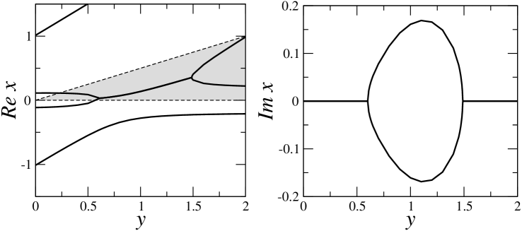
Figure 1: Real (left panel) and imaginary (right panel) parts of the four roots of the dispersion relation (30) for model parameters $a^{2}=0.0249$ and $b^{2}=0.0379$. For these parameters the quartic dispersion relation has four real roots for both $y=0$ and $y=2$, while it has two real roots and a complex conjugate pair for $y$ in the range $0.6<y<1.5$. In this range, the two-stream instability is operating. The grey area corresponds to $0\leq\mbox{Re }x\leq 1/2$ which is contained in the range of the instability criteria discussed in Section IIC.

We have thus established that the two-stream instability may, in principle, operate in superfluids. Our example indicates the existence of a lower limit of the background flow for the instability. This turns out to be a generic feature. In contrast, the plasma two-stream instability can operate at arbitrarily slow flows. An ideal plasma is unstable to sufficiently long wavelengths for any given $v_{0}$. In reality, however, one must also account for dissipative mechanisms. In the case of real plasmas one finds that the so-called Landau damping stabilizes the longest wavelengths (Anderson et al, 2001). Thus the two-stream instability sets in below a critical wavelength in more realistic plasma models, and there is typically (just like in the present case) a range of flows for which the instability is present. We will discuss the effects of dissipation on the superfluid two-stream instability briefly in Section IV.

2.3 Necessary criteria for instability

It is useful to consider whether we can derive a necessary condition for the two-stream instability.To approach this problem in full generality would likely be quite complicated, but we can make good progress for the simple one-dimensional toy problem discussed above.

We begin by multiplying the Euler equation (14) for the neutrons by the complex conjugate $\delta v^{*}_{\mathrm{n}}$. This leads to (after also using the continuity equations to replace the perturbed number densities)

$$\left(\omega-kv_{0}-{k^{2}c_{\mathrm{n}}^{2}\over\omega-kv_{0}}\right)|\delta v_{\mathrm{n}}|^{2}={\cal C}{k^{2}n_{\mathrm{p}}\over n_{\mathrm{n}}\omega}\delta v^{*}_{\mathrm{n}}\delta v_{\mathrm{p}}\ .$$ (34)

Similarly, we obtain from the second Euler equation (15)

$$\left(\omega-{k^{2}c_{\mathrm{p}}^{2}\over\omega}\right)|\delta v_{\mathrm{p}}|^{2}={\cal C}{k^{2}\over\omega-kv_{0}}\delta v^{*}_{\mathrm{p}}\delta v_{\mathrm{n}}\ .$$ (35)

Next we combine these two equations to get

$${\cal L}={n_{\mathrm{n}}\over n_{\mathrm{p}}}\sigma_{p}\left(\sigma_{p}-v_{0}-{c_{\mathrm{n}}^{2}\over\sigma_{p}-v_{0}}\right)|\delta v_{\mathrm{n}}|^{2}+(\sigma_{p}-v_{0})\left(\sigma_{p}-{c_{\mathrm{p}}^{2}\over\sigma_{p}}\right)|\delta v_{\mathrm{p}}|^{2}={\cal C}\left(\delta v^{*}_{\mathrm{n}}\delta v_{\mathrm{p}}+\delta v^{*}_{\mathrm{p}}\delta v_{\mathrm{n}}\right)$$ (36)

where we have introduced the pattern speed $\sigma_{p}$. From this expression we see that the imaginary part of the left-hand side must vanish, so we should have Im ${\cal L}=0$. Allowing the pattern speed to be complex, i.e. using $\sigma_{p}=\sigma_{R}+i\sigma_{I}$ we find that the following condition must be satisfied

$$\mbox{Im }{\cal L}=\sigma_{R}\sigma_{I}\left\{{n_{\mathrm{n}}\over n_{\mathrm{p}}}\left[2-{v_{0}\over\sigma_{R}}\left(1-{c_{\mathrm{n}}^{2}\over|\sigma_{p}-v_{0}|^{2}}\right)\right]|\delta v_{\mathrm{n}}|^{2}+\left[2-{v_{0}\over\sigma_{R}}\left(1+{c_{\mathrm{p}}^{2}\over|\sigma_{p}|^{2}}\right)\right]|\delta v_{\mathrm{p}}|^{2}\right\}=0\ .$$ (37)

If we are to have an unstable mode, $\sigma_{I}\neq 0$, the frequency clearly must be such that the factors multiplying the absolute values of the two velocities have different signs.

Let us first consider the case when the factor multiplying $|\delta v_{\mathrm{n}}|^{2}$ is negative. Then we find that an instability is only possible if ${\sigma_{R}/v_{0}}<0$, and the following condition is satisfied:

$$0<\left|{\sigma_{R}\over v_{0}}\right|<{1\over 2}\left({c_{\mathrm{n}}^{2}\over|\sigma_{p}-v_{0}|^{2}}-1\right)\ .$$ (38)

This shows that we must have

$${c_{\mathrm{n}}\over|v_{0}|}>\left|{\sigma_{p}\over v_{0}}-1\right|>\left|{\sigma_{R}\over v_{0}}-1\right|=\left|{\sigma_{R}\over v_{0}}\right|+1>1$$ (39)

which constrains the permissible frequencies to the range $|\sigma_{R}|<c_{\mathrm{n}}-|v_{0}|$. Thus we see that the flow must be subsonic, i.e. $|v_{0}|<c_{\mathrm{n}}$.

In the case when the factor multiplying $|\delta v_{\mathrm{p}}|^{2}$ is negative we can only have an instability if ${\sigma_{R}/v_{0}}>0$. We also require

$$0<{\sigma_{R}\over v_{0}}<{1\over 2}\left(1+{c_{\mathrm{p}}^{2}\over|\sigma_{p}|^{2}}\right)<{1\over 2}\left(1+{c_{\mathrm{p}}^{2}\over\sigma_{R}^{2}}\right)\quad\mbox{ if }\quad|\sigma_{p}-v_{0}|^{2}<c_{\mathrm{n}}^{2}$$ (40)

or

$${1\over 2}\left(1-{c_{\mathrm{n}}^{2}\over|\sigma_{R}-v_{0}|^{2}}\right)<{1\over 2}\left(1-{c_{\mathrm{n}}^{2}\over|\sigma_{p}-v_{0}|^{2}}\right)<{\sigma_{R}\over v_{0}}<{1\over 2}\left(1+{c_{\mathrm{p}}^{2}\over\sigma_{R}^{2}}\right)\quad\mbox{ if }\quad|\sigma_{p}-v_{0}|^{2}>c_{\mathrm{n}}^{2}\ .$$ (41)

For the example illustrated in Figure 1, the condition that must be satisfied is (40). It is useful to notice two things about this criterion. First of all, any unstable mode for which $\sigma_{R}>c_{\mathrm{p}}$ must lie in the range $0<c_{\mathrm{p}}<\sigma_{R}<v_{0}$. Secondly, when $\sigma_{R}>>c_{\mathrm{p}}$ the permissible range will be well approximated by $0<\sigma_{R}<v_{0}/2$, cf. Figure 2. As is clear from Figure 1 the unstable modes satisfy this last, and most severe, criterion.

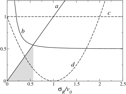
Figure 2: An illustration of the instability criterion (40) which is relevant for the example considered in Section IIB. This example is constructed by introducing $z=\sigma_{R}/v_{0}$, and then showing the four curves: $a(z)=z$, $b(z)=(1+\gamma^{2}/z^{2})/2$, $c(z)=1$ and $d(z)=(z-1)^{2}$. Here we have taken $c_{\mathrm{n}}^{2}/v_{0}^{2}=1$ and $\gamma^{2}=c_{\mathrm{p}}^{2}/c_{\mathrm{n}}^{2}=0.0379$. Criterion (40) is satisfied when $d<c$ and $a<b$ (in the grey area). The corresponding range is well approximated by $0<\sigma_{R}/v_{0}<1/2$.

It is worth noting that the instability can be discussed in terms of a simple energy argument [see Casti et al (1998) and Pierce (1974) for similar discussions in other contexts]. After averaging over several wavelengths, the kinetic energy of the protons is

$$E_{\mathrm{p}}\approx{m_{\mathrm{p}}n_{\mathrm{p}}\delta v_{\mathrm{p}}^{2}\over 2}>0\ .$$ (42)

Meanwhile we get for the neutrons

$$E_{\mathrm{n}}\approx{m_{\mathrm{n}}\over 2}(n_{\mathrm{n}}+\delta n_{\mathrm{n}})(v_{0}+\delta v_{\mathrm{n}})^{2}$$ (43)

which leads to

$$E_{\mathrm{n}}\approx{m_{\mathrm{n}}n_{\mathrm{n}}\over 2}\left[v_{0}^{2}+{\omega+kv_{0}\over\omega-kv_{0}}\delta v_{\mathrm{n}}^{2}\right]$$ (44)

from which we see that the energy in the perturbed flow is smaller than the energy in the unperturbed case, which means that we can associate the wave with a “negative energy”, when

$$-v_{0}<{\omega\over k}<v_{0}\ ,\quad\mbox{i.e. }\quad-v_{0}<\sigma_{R}<v_{0}\ .$$ (45)

A wave that satisfies $0<\sigma_{R}<v_{0}$ moves forwards with respect to the protons but backwards according to an observer riding along with the unperturbed neutron flow. As we have seen above, the unstable modes in our problem satisfy this criterion and hence it is easy to explain the physical conditions required for the two-stream instability to be present.

2.4 Results for a simple model equation of state

Having established that the two-stream instability may be present in superfluids, we want to assess to what extent one should expect this mechanism to play a role for astrophysical neutron stars. To do this we will consider two particular equations of state. The results we obtain illustrate different facets of what we expect to be a rich problem.

We begin by making contact with our recent analysis of rotating superfluid models (Prix et al, 2002) as well as the study of oscillating non-rotating stars by Prix & Rieutord (2002). From the definitions above we have

$$a^{2} = {n_{\mathrm{p}}\over n_{\mathrm{n}}}{{\cal S}_{\mathrm{n}\mathrm{p}}^{2}\over{\cal S}_{\mathrm{p}\mathrm{p}}^{2}}\ ,$$ (46)

$$b^{2} = {n_{\mathrm{p}}\over n_{\mathrm{n}}}{{\cal S}_{\mathrm{n}\mathrm{n}}\over{\cal S}_{\mathrm{p}\mathrm{p}}}\ .$$ (47)

We combine these results with the explicit structure matrix given in eq. (144) of Prix et al (2002), which is based on a simple “analytic” equation of state. This leads to

$$a^{2} = {n_{\mathrm{p}}\over n_{\mathrm{n}}}\sigma^{2}\ ,$$ (48)

$$b^{2} = 1+{\sigma(1-2x_{\mathrm{p}})\over 1-x_{\mathrm{p}}}\ ,$$ (49)

where $x_{\mathrm{p}}=n_{\mathrm{p}}/(n_{\mathrm{p}}+n_{\mathrm{n}})$ is the proton fraction, and $\sigma$ is defined by

$$\sigma={{\cal S}_{\mathrm{n}\mathrm{p}}\over{\cal S}_{\mathrm{p}\mathrm{p}}}\ .$$ (50)

As discussed by Prix et al (2002), $\sigma$ is related to the “symmetry energy” of the equation of state, cf. Prakash et al (1988).

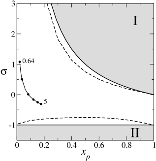
Figure 3: An illustration of the various domains of instability for the simple “analytic” equation of state of Prix et al (2002). An absolute instability (see discussion in the main text) is active in the grey areas (also labeled I and II). The two-stream instability is, in principle, relevant in the remaining parameter space. The dashed curves indicate the onset of instability when the relative flow is equal to the neutron sound speed $(y=1$). For slower flows, these critical curves approach the absolute instability regions. The region where the two-stream instability may operate in physical flows therefore lies between each dashed curve and the nearest grey area. For comparison we also indicate the curve in the $x_{\mathrm{p}}-\sigma$ plane traced out by the PAL equation of state (discussed in Section IIE) as the density is varied from that near the crust/core interface ($u=0.64$) to five times that of nuclear saturation $(u=5)$.

The instability regions for this model equation of state are illustrated in Figure 3. A key feature of this figure is the presence of regions of “absolute instability”. This happens when $a^{2}>b^{2}$. Then there exist unstable solutions already for vanishing background flow, $y=0$. That this is the case is easy to see. Consider $(\ref{fxy})$ in the limit $y=0$. In the limit we can solve directly for $x^{2}$:

$$x^{2}={1+b^{2}\over 2}\pm\sqrt{\left({1+b^{2}\over 2}\right)^{2}-b^{2}+a^{2}}$$ (51)

from which it is easy to see that one of the roots for $x^{2}$ will be negative if $a^{2}>b^{2}$. Hence, one of the roots to the quartic (30) will be purely imaginary.

The physics of this instability is quite different from the two-stream instability that is the main focus of this paper. Yet it is an interesting phenomenon. From the above relations we find that $a^{2}<b^{2}$ corresponds to

$${\cal S}_{\mathrm{n}\mathrm{n}}{\cal S}_{\mathrm{p}\mathrm{p}}>{\cal S}_{\mathrm{n}\mathrm{p}}^{2}\ .$$ (52)

In the discussion by Prix et al (2002) it was assumed that “reasonable” equations of state ought to satisfy this condition. We expected this to be the case since the structure matrix would not be invertible if its determinant were to vanish at some point. We now see that this constraint has a strong physical motivation: The condition is violated when $a^{2}>b^{2}$, i.e. when we have an absolute instability. The regions where this instability is active are indicated by the grey areas in Figure 3.

2.5 Results for the PAL equation of state

In order to strengthen the argument that the two-stream instability may operate in astrophysical neutron stars, we have considered a “realistic” equation of state due to Prakash, Ainsworth and Lattimer (PAL) (1988). The advantage of this model is that it is relatively simple. In particular, it leads to analytical expressions for the various quantities needed in our analysis. The energy density of the baryons for the PAL equation of state can be written

$${\cal E}(n_{\mathrm{n}},n_{\mathrm{p}})=\left(n_{\mathrm{n}}+n_{\mathrm{p}}\right)\left[E_{0}(u)+S(u)(1-2x_{\mathrm{p}})^{2}\right]\ ,$$ (53)

where $E_{0}$ corresponds to the energy per nucleon, $S$ corresponds to the “symmetry energy” (and is closely related to $\sigma$ in the “analytic” equation of state discussed above), and $u=(n_{\mathrm{n}}+n_{\mathrm{p}})/n_{0}$ with $n_{0}=0.16\ {\rm fm}^{-3}$ the nuclear saturation density. $E_{0}$ takes the following form:

$$E_{0}(u)=A_{0}u^{2/3}+B_{0}u+C_{0}u^{\sigma}+3\sum_{i=1}^{2}C_{i}\alpha_{i}^{-3}\left[\alpha_{i}u^{1/3}-\arctan\left(\alpha_{i}u^{1/3}\right)\right]\ ,$$ (54)

with $A_{0}=22.11$ MeV, $B_{0}=220.47$ MeV, $C_{0}=-213.41$ MeV, $\sigma=0.927$, $C_{1}=-83.84$ MeV, $C_{2}=23.0$ MeV, $\alpha_{1}=2/3$, and $\alpha_{2}=1/3$. The symmetry term is

$$S(u)=A_{S}\left[u^{2/3}-F(u)\right]+S_{0}F(u)\ ,$$ (55)

with $A_{S}=12.99$ MeV and $S_{0}=30$ MeV. Here $F(u)$ is a function satisfying $F(1)=1$ which is supposed to simulate the behaviour of the potentials used in theoretical calculations. In our study we have only considered $F(u)=u$, which is one of four possibilities discussed by Prakash et al (1988).

We further need to account for the energy contribution of the electrons, which is important since the electrons are highly relativistic inside neutron stars. Hence, they can obtain high (local) Fermi energies which may be comparable with the proton (local) Fermi energies. Considering only the electrons, the leptonic contribution to the energy density is given by (in units where the speed of light is unity) (Shapiro & Teukolsky, 1983)

$${\cal E}_{\mathrm{e}}={m_{\mathrm{e}}\over\lambda_{\mathrm{e}}^{3}}\chi\left(\chi^{F}_{\mathrm{e}}\right)\ ,$$ (56)

where $m_{\mathrm{e}}=m_{\mathrm{b}}/1836$ is the electron mass (in terms of the baryon mass $m_{\mathrm{b}}$), $\lambda_{\mathrm{e}}=\hbar/m_{\mathrm{e}}$ is the electron Compton wavelength, and

$$\chi(x)={1\over 8\pi^{2}}\left(x\left[1+x^{2}\right]^{1/2}\left[1+2x^{2}\right]-{\rm ln}\left[x+\left(1+x^{2}\right)^{1/2}\right]\right)\ ,$$ (57)

$$\chi^{F}_{\mathrm{e}}=1836\left(3\pi^{2}\left[{\hbar\over m_{b}}\right]^{3}\right)^{1/3}n_{\mathrm{p}}^{1/3}\ .$$ (58)

In doing this calculation we have assumed local charge neutrality, i.e. $n_{\mathrm{e}}=n_{\mathrm{p}}$. The above energy term is added linearly in the equation of state.

Having obtained an expression for the total energy as a function of the density, we can derive explicit expressions for all quantities needed to discuss the two-stream instability. First we need to determine the proton fraction $x_{\mathrm{p}}$. We do this by assuming that the star is in chemical equilibrium, i.e.

$$\mu^{\mathrm{n}}=\mu^{\mathrm{p}}+\mu^{\mathrm{e}}\,.$$ (59)

Solving (59) for $x_{\mathrm{p}}$ provides us with the proton fraction as a function of $u$. Given this, and the relevant partial derivatives of ${\cal E+E}_{\mathrm{e}}$ we can readily evaluate the symmetry energy and well as the sound speeds $c_{\mathrm{n}}^{2}$, $c_{\mathrm{p}}^{2}$ and the chemical coupling parameter ${\cal C}$. With this data we can determine the two parameters $a^{2}$ and $b^{2}$ which are needed if we want to solve the local dispersion relation (30). The results we obtain for the proton fraction and the symmetry energy are indicated in Figure 3. We consider the range from $u=0.64$, presumed to correspond to the core-crust boundary, to $u=5$ which represents the deep core of a realistic neutron star. The corresponding results for the two-stream instability are shown in Figure 4. From this figure we can see that the two-stream instability may operate (albeit at comparatively large relative flows) in the region immediately below the crust. Finally, we find that the conditions at the core-crust interface are such that $a^{2}=0.0249$ and $b^{2}=0.0379$. These are the values we chose for the example in Section IIB and hence the results shown in Figure 1 correspond to a physically realistic model.

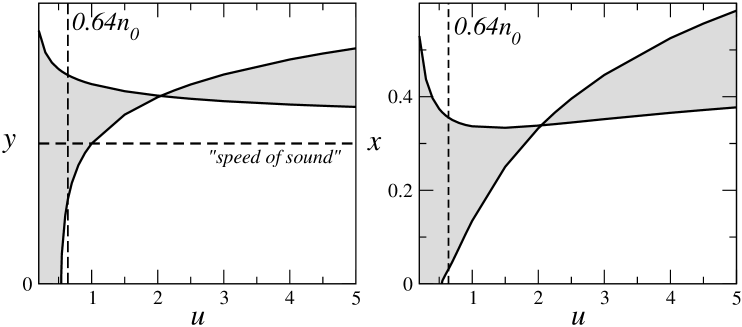
Figure 4: Two-stream instability results for the PAL equation of state. Left panel: The region where the two-stream instability is present (grey area) is shown as a function of the density parameter $u$. We indicate the location of the core-crust boundary ($u\approx 0.64$) by a vertical dashed line. Our model is only relevant for the core fluid, i.e. to the right of the vertical line. Finally, the horizontal dashed line indicates when the relative flow is equal to the (neutron) sound speed. We expect the superfluid degeneracy to be broken beyond this level, so an instability located above this line is unlikely to have physical relevance. The results indicate that there may be a region of instability immediately below the crust. Right panel: The corresponding oscillation frequencies. Particularly notable is the point near $u=2$ where the two critical curves cross. At this point the symmetry energy $\sigma$ changes sign, cf. Fig. 3, and there exist a particular density such that the two fluids are uncoupled, cf. (31).

3 Rotating shells: A connection with pulsar glitches?

The fact that a superfluid neutron star may, in principle, exhibit the two-stream instability does not necessarily prove that this mechanism will be astrophysically relevant. Yet, it is an intriguing possibility given that the mechanism underlying the enigmatic glitches observed in dozens of pulsars remains poorly understood. One plausible astrophysical role for the superfluid two-stream instability would be in this context: Perhaps this instability serves as trigger mechanism for large pulsar glitches?

3.1 Dispersion relation for rotating shells

Our aim in this Section is to construct a toy problem that allows us to investigate a possible connection between the two-stream instability and pulsar glitches. A suitably simple problem corresponds to two fluids, allowed to rotate at different rates, confined within an infinitesimally thin spherical shell. By assuming that the shell is infinitesimal we ignore radial motion, i.e. we restrict the permissible perturbations of this system is such a way that the perturbed velocities must take the form

$$\delta\vec{v}_{X}=-{1\over R\sin\theta}U^{X}_{lm}(t)\partial_{\varphi}Y^{m}_{l}\hat{e}_{\theta}+{1\over R}U^{X}_{lm}(t)\partial_{\theta}Y^{m}_{l}\hat{e}_{\varphi}$$ (60)

where $Y^{m}_{l}(\theta,\varphi)$ are the spherical harmonics and $R$ is the radius $R$ of the shell. This means that the system permits only toroidal mode-solutions. In other words, all oscillation modes of this shell model are closely related to the inertial r-modes of rotating single fluid objects (Papaloizou & Pringle, 1978; Provost et al, 1981).

The perturbation equations for the configuration we consider have been derived in a different context and the complete calculation will be presented elsewhere (Andersson et al, 2002). Our primary interest here concerns whether the modes of this system may suffer the two-stream instability. The presence of the instability in this toy problem would be a strong indication that it will also be relevant when the shells are “thick” and radial motion is possible. That is, when we consider a rotating star that contains a partially decoupled superfluid either in the inner crust or the core.

As discussed in Section IIC, the two-stream instability can be understood in terms of negative energy waves. In the current problem, the criterion for waves to carry negative energy according to one fluid but positive energy according to the other fluid is that the mode pattern speed [we are assuming a decomposition $\exp(i\omega t+im\varphi)$]

$$\sigma_{p}=-{\omega\over m}$$ (61)

lies between the two (uniform) rotation rates. In other words, a necessary condition for instability is

$$\Omega_{\mathrm{p}}<\sigma_{p}<\Omega_{\mathrm{n}}$$ (62)

where we have assumed that the superfluid neutrons lag behind the charged component, as is expected in a spinning down pulsar.

After a somewhat laborious calculation, see Andersson et al (2002) for details, one finds that the dispersion relation for the toroidal two-fluid modes of the shell problem is

$$\left\{-l\left(l+1\right)(1-\varepsilon_{\mathrm{n}})\left[\omega+m\Omega_{\mathrm{n}}\right]+2m\Omega_{\mathrm{n}}+m\varepsilon_{\mathrm{n}}\left[2-l\left(l+1\right)\right]\left[\Omega_{\mathrm{p}}-\Omega_{\mathrm{n}}\right]\right\}$$ (63)

$$\times\left\{-l\left(l+1\right)(1-\varepsilon_{\mathrm{p}})\left[\omega+m\Omega_{\mathrm{p}}\right]+2m\Omega_{\mathrm{p}}+m\varepsilon_{\mathrm{p}}\left[2-l\left(l+1\right)\right]\left[\Omega_{\mathrm{n}}-\Omega_{\mathrm{p}}\right]\right\}$$ (64)

$$-\left\{l\left(l+1\right)\right)^{2}\varepsilon_{\mathrm{n}}\varepsilon_{\mathrm{p}}\left(\omega+m\Omega_{\mathrm{n}}\right)\left(\omega+m\Omega_{\mathrm{p}}\right\}=0\ .$$ (65)

This equation should be valid under the conditions in the outer core of a mature neutron star, where superfluid neutrons are permeated by superconducting protons.

We rewrite this dispersion relation in terms of the entrainment parameter used by Prix et al (2002), namely

$$\varepsilon=\varepsilon_{\mathrm{p}}={2\alpha\over\rho_{\mathrm{p}}}\ ,$$ (66)

the frequency as measured with respect to the rotation of the protons,

$$\kappa={\omega\over m\Omega_{\mathrm{p}}}\ ,$$ (67)

and a dimensionless measure of the relative rotation,

$$\Lambda={\Omega_{\mathrm{n}}\over\Omega_{\mathrm{p}}}\ .$$ (68)

With these definitions we get

$$\left\{l(l+1)[1-x_{\mathrm{p}}(1+\varepsilon)](\kappa+\Lambda)-2(1-x_{\mathrm{p}})\Lambda+x_{\mathrm{p}}\varepsilon(l-1)(l+2)(1-\Lambda)\right\}$$

$$\times\left\{l(l+1)[1-\varepsilon](\kappa+1)-2-\varepsilon(l-1)(l+2)(1-\Lambda)\right\}$$

$$-[l(l+1)]^{2}x_{\mathrm{p}}\varepsilon^{2}(\kappa+\Lambda)(\kappa+1)=0\ .$$ (69)

In terms of these new variables a mode would satisfy the necessary instability criterion (62) if $\kappa$ is such that

$$-\Lambda<\kappa<-1\ .$$ (70)

As we will now establish, there exist modes that satisfy this criterion for reasonable parameter values.

3.2 An extreme example: The quadrupole modes

Let us first consider the case of quadrupole oscillations, i.e. take $l=2$. Typical results for this case are shown in Figures 5 and 6. The first figure illustrates the regions of the $x_{\mathrm{p}}-\varepsilon$ parameter space for which an instability is present in the case when (i) the neutrons rotate at a rate that is 90% faster than that of the charged component, and (ii) the neutrons lag behind by the same fraction. The second figure shows the mode-frequencies corresponding to the second case [simply obtained by solving the quadratic (69)] for the particular value $x_{\mathrm{p}}=0.05$. This figure shows the presence of unstable modes within the range of values for $\varepsilon$ that we take to be physically realistic (Prix et al, 2002): $0.4\leq\varepsilon\leq 0.7$. From this figure we immediately deduce two things. First, we see that the unstable modes indeed satisfy the criterion (70). Secondly, the unstable modes may have imaginary parts as large as Im $\kappa\approx 0.15$. It is useful to ask what this implies for the growth time of the instability. Since our results only depend on the azimuthal index $m$ through the scaling

$$\mbox{Im }\omega=m\Omega_{\mathrm{p}}\mbox{ Im }\kappa$$ (71)

we see that the fastest growth time corresponds to the $m=l$ modes. The e-folding time for the instability follows from

$$t_{e}={1\over m\Omega_{\mathrm{p}}\mbox{ Im }\kappa}={1\over 2\pi m\mbox{ Im }\kappa}P\mbox{ s}$$ (72)

where $P$ represents the observed rotation period of the pulsar (presumably corresponding to the rotation of the charged component, i.e. $P/2\pi/\Omega_{\mathrm{p}}$).

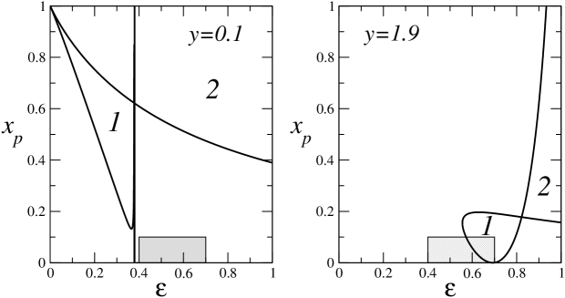
Figure 5: Instability regions for the shell problem. We show results for $l=2$ and relative rotation such that the neutrons rotate 90% slower (left frame) or faster (right frame) than the protons. The two-stream instability operates in regions 1-2. The grey box corresponds to the “physically reasonable” part of parameter space (for the core of a neutron star).

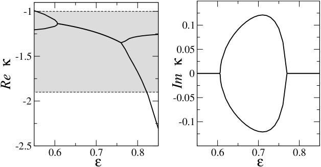
Figure 6: Real and imaginary parts (left and right frame, respectively) of the mode frequencies for $l=2$, $\Lambda=1.9$ and $x_{\mathrm{p}}=0.05$. The corresponding instability region can be deduced from the right panel of Fig. 5. The grey area in the left frame indicates the region where an instability is permissible according to (70).

The above example shows that the two-stream instability does indeed operate in this shell problem. In fact, the analysis goes beyond the local analysis of the plane parallel problem in Section IIB since we have now solved for the actual unstable modes (satisfying the relevant boundary conditions). We see that, as expected for a dynamical instability, the growth time of an unstable mode may be very short. However, the relative rotation rates required to make the quadrupole modes unstable in the range $0<x_{\mathrm{p}}<1$ and $0<\varepsilon<1$ are likely far too large to be physically attainable. In this sense the results shown in Figs. 5–6 are, despite being instructive, somewhat extreme.

3.3 A realistic mechanism for triggering pulsar glitches?

A quantity of key importance for this discussion is the rotational lag between the two components. In order to be able to argue that the two-stream instability is relevant for pulsar glitches we need to consider lags that may actually occur in astrophysical neutron stars. To estimate the size of the rotational lag required to “explain” the observed glitches we assume that a glitch corresponds to a transfer of angular momentum from a partially decoupled superfluid component (index $\mathrm{n}$) to the bulk of the star (index $\mathrm{p}$). Then we have

$$I_{\mathrm{n}}|\Delta\Omega_{\mathrm{n}}|\approx I_{\mathrm{p}}\Delta\Omega_{\mathrm{p}}\rightarrow\Delta\Omega_{\mathrm{p}}\approx{I_{\mathrm{n}}\over I_{\mathrm{p}}}|\Delta\Omega_{\mathrm{n}}|$$ (73)

where $I_{X}$ are the two moments of inertia. Now assume that the decoupled component corresponds 1% of the total moment of inertia, eg. the superfluid neutrons in the inner crust or a corresponding amount of fluid in the core. This would mean that $I_{\mathrm{n}}\sim 10^{-2}I_{\mathrm{p}}$, and we have

$$\Delta\Omega_{\mathrm{p}}\approx 10^{-2}|\Delta\Omega_{\mathrm{n}}|\ .$$ (74)

Combine this with the observations of large Vela glitches to get

$${\Delta\Omega_{\mathrm{p}}\over\Omega_{\mathrm{p}}}\approx 10^{-2}{|\Delta\Omega_{\mathrm{n}}|\over\Omega_{\mathrm{p}}}\sim 10^{-6}\ .$$ (75)

In other words, we must have

$$|\Delta\Omega_{\mathrm{n}}|\approx 10^{-4}\Omega_{\mathrm{p}}\ .$$ (76)

If we assume that the glitch brings the two fluids back into co-rotation, then we have $\Delta\Omega_{\mathrm{n}}=\Omega_{\mathrm{n}}-\Omega_{\mathrm{p}}=\Delta\Omega$ and we see that the two rotation rates will maximally differ by one part in $10^{4}$ or so. Rotational lags of this order of magnitude have often been discussed in the context of glitches. Even though the key quantity in models invoking catastrophic vortex unpinning in the inner crust — the pinning strength — is very uncertain, and there have been suggestions that the pinning force is too weak to allow a build up of the required rotational lag (Jones, 1998), typical values considered are consistent with our rough estimate. In addition, frictional heating due to a difference in the rotation rates of the bulk of a neutron star and a superfluid component has been discussed as a possible explanation for the fact that old isolated pulsars seem to be somewhat hotter than expected from standard cooling models (Shibazaki & Lamb, 1989; Larson & Link, 1999). Larson & Link (1999) argue that a lag of

$${\Delta\Omega\over\Omega_{\mathrm{p}}}\approx(3.2\times 10^{-4}-9.5\times 10^{-3})\times\left(0.1\mbox{ s}\over P\right)$$ (77)

could explain the observational data. Finally, the presence of rotational lags of the proposed magnitude is supported by a statistical analysis of 48 glitches in 18 pulsars (Lyne et al, 2000). This study suggests that the critical rotational lag at which a glitch occurs is

$${\Delta\Omega\over\Omega_{\mathrm{p}}}\approx 5\times 10^{-4}\ .$$ (78)

In order to make our shell model problem more realistic we consider the case when the superfluid neutrons lag behind the superconducting protons, and take $\Delta\Omega/\Omega_{\mathrm{p}}=5\times 10^{-4}$, or $\Lambda=1.0005$, as a representative value. With this rotational lag, we see from (70) that the unstable modes must be such that $-1.0005<\kappa<-1$. A series of results for this choice of parameters are shown in Figures 7-9.

Figure 7 illustrates the fact that, if we decrease the rotational lag then the two-stream instability will not be active (in the interesting region of parameter space) for low values of $l$. For a smaller rotational lag the instability acts on a shorter length scale. For $\Lambda=1.0005$ we find that we must have $l>65$ in order for there to be a region of instability in the part of the $x_{\mathrm{p}}-\varepsilon$ plane shown in Figure 7. This means that the instability only operates on length scales shorter than $\pi R/l\approx 500$ m (if we take the shell radius to be $R=10$ km).

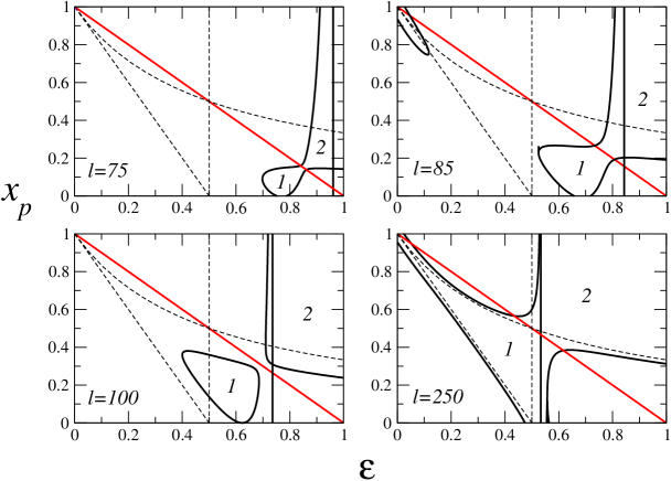
Figure 7: The two-stream instability regions (labeled 1 and 2) for the case when the superfluid neutrons lag behind the superconducting protons in such a way that $\Delta\Omega/\Omega_{\mathrm{p}}=5\times 10^{-4}$ or $\Lambda=1.0005$. We show results for four different values of $l$. There are no unstable modes in this part of parameter space unless $l>65$. Recall that $x_{\mathrm{p}}<0.1$ and $0.4\leq\varepsilon\leq 0.7$ would be reasonable parameter values for a neutron star core. The grey diagonal line represents the singularity discussed in Section IIID and the dashed curves indicate the instability regions in the large $l$ limit.

Figure 8 shows the real part of the mode frequencies for $l=100$ and various values of $x_{\mathrm{p}}$. From this figure we can see that the instability always occur in the region suggested by the instability condition (70), i.e. two real frequency modes never merge to give rise to a complex conjugate pair of solutions outside the grey areas indicated in the various panels of Figure 8. The imaginary parts for $l=100$ and the various values of $x_{\mathrm{p}}$ considered in Figure 8 are shown in Figure 9. From this figure we see that the imaginary part of $\kappa$ typically reaches values of order $10^{-4}$. In fact, by comparing similar results for different values of $l$ we have found that the largest attainable imaginary part of $\kappa$ varies by less than one order of magnitude as $l$ increases from 100 to 1000. Thus we estimate that the typical instability growth time for $\Lambda=1.0005$ will be

$$t_{e}\approx{10^{4}\over m}{P\over 2\pi}\mbox{ s}\ .$$ (79)

For a star rotating at the rate of the Vela pulsar, $P=89$ ms, we would have $t_{e}\approx 1.4$ s for $l=m=100$. Interestingly, this predicted growth time is significantly shorter than the resolved rise time of a large Vela glitch $t_{\rm glitch}<40$ s (Dodson et al, 2002).

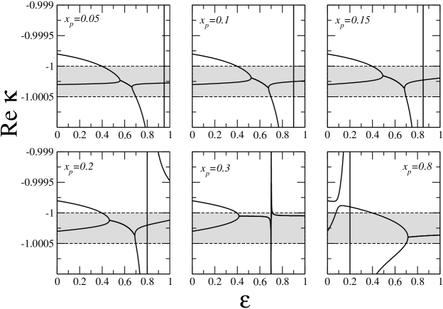
Figure 8: Mode frequencies (represented by Re $\kappa$) as function of the entrainment parameter $\varepsilon$ for $l=100$, $\Lambda=1.0005$ and various values of $x_{\mathrm{p}}$. The range in which an instability is permissible [according to (70)] is indicated by the grey areas.

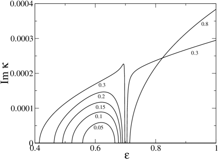
Figure 9: The imaginary part Im $\kappa$ (determining the growth rate) of the unstable modes for $\Lambda=1.0005$ and $l=100$ is shown as a function of $\varepsilon$ for several different values of $x_{\mathrm{p}}$ (as indicated in the figure). Essentially, these results represent horizontal cuts through the frames in Figure 7.

3.4 Approximate results: The large $l$ limit

The results obtained above indicate that the two-stream instability is likely to act on modes with rather short wavelengths. Given this it makes sense to consider the large $l$ limit in more detail. Keeping only the leading order term (proportional to $l^{4}$) in (69) we have the dispersion relation

$$(1-\varepsilon-x_{\mathrm{p}})\kappa^{2} + \left[1-2\varepsilon-x_{\mathrm{p}}+2x_{\mathrm{p}}\varepsilon+(1-x_{\mathrm{p}}-2x_{\mathrm{p}}\varepsilon)\Lambda\right]\kappa$$ (80)

$$+ (1-2\varepsilon-x_{\mathrm{p}})\Lambda+\varepsilon x_{\mathrm{p}}+\varepsilon(1-x_{\mathrm{p}})\Lambda^{2}-2x_{\mathrm{p}}\varepsilon^{2}(1-\Lambda)^{2}=0\ .$$

We can readily write down the solutions to this quadratic:

$$\kappa_{\pm} = {1\over 2(1-x_{\mathrm{p}}-\varepsilon)}\left\{1-2\varepsilon-x_{\mathrm{p}}+2\varepsilon x_{\mathrm{p}}+(1-x_{\mathrm{p}}-2x_{\mathrm{p}}\varepsilon)\Lambda\right.$$ (81)

$$\pm \left.(1-\Lambda)\left[(1-2\varepsilon)(1-2\varepsilon-x_{\mathrm{p}})(1-x_{\mathrm{p}}-2\varepsilon x_{\mathrm{p}})\right]^{1/2}\right\}\ .$$

It turns out that we can learn a lot about the problem from this expression. The most obvious feature is the fact that $\kappa_{\pm}$ have a singularity when $1-x_{\mathrm{p}}-\varepsilon=0$. It is straightforward to show that one of the roots will become infinite at this point, while the second root becomes:

$$\kappa={1\over 1-2x_{\mathrm{p}}}\left[\Lambda-x_{\mathrm{p}}(1+\Lambda)+2x_{\mathrm{p}}\varepsilon(1-\Lambda)\right]\ .$$ (82)

For the examples shown in Figure 7 this special case corresponds to the intersection between the instability domain and the diagonal line $1-x_{\mathrm{p}}-\varepsilon=0$, as indicated in Figure 7.

It is also straightforward to deduce the regions of instability from the sign of the argument of the square-root. We see that we will have an unstable mode when

$$\varepsilon<{1\over 2}\qquad\mbox{and}\qquad 1-2\varepsilon<x_{\mathrm{p}}<{1\over 1+2\varepsilon}\qquad\mbox{Region 1}$$ (83)

or

$$\varepsilon>{1\over 2}\qquad\mbox{and}\qquad x_{\mathrm{p}}>{1\over 1+2\varepsilon}\qquad\mbox{Region 2}\ .$$ (84)

These regions are also indicated in Figure 7. Out of these two possible instability regions, the first is most likely to be relevant for neutron stars since it allows the instability to be present already for small proton fractions.

Finally, we can use (81) to show the existence of an extremum at

$$\varepsilon={1\over 8}(\sqrt{17}-1)\approx 0.39\quad\ ,\quad x_{\mathrm{p}}={1\over 4}{\sqrt{17}+7\over\sqrt{17}+3}\approx 0.39\ .$$

The corresponding imaginary part of $\kappa$ would represent the fastest possible growth time for an unstable mode located in region 1 of Figure 7. This leads to the estimate

$$\mbox{Im }\kappa\leq 0.24(\Lambda-1)$$ (85)

or an estimate of the shortest growth time:

$$t\approx{6.7\times 10^{-2}\over l}\left({\Delta\Omega\over\Omega_{\mathrm{p}}}\right)^{-1}\left({P\over 0.1\mbox{ s}}\right)\mbox{ s}$$ (86)

which agrees well with the result we previously obtained for $l=m=100$. Hence, this simple formula can be used to estimate the fastest growth rate of the two-stream instability in our shell model for different parameter values.

4 Discussion

In this paper we have introduced the superfluid two-stream instability: A dynamical instability analogous to that known to operate in plasmas (Anderson et al, 2001), which sets in once the relative flow between the two components of the system reaches a critical level. We have studied this instability for two different model problems. First we analysed a local dispersion relation derived for the case of a background such that one fluid was at rest while the other had a constant flow rate. This provided a proof of principle of the existence of the two-stream instability for superfluids. Our analysis was based on the two-fluid equations that have been used to model the dynamics of the outer core of a neutron star, where superfluid neutrons are expected to coexist with superconducting protons and relativistic electrons. These equations are analogous to the Landau model for superfluid Helium , and should also (after some modifications to incorporate elasticity and possible vortex pinning) be relevant for the conditions in the inner crust of a mature neutron star. Thus we expect the two-stream instability to be generic in dynamical superfluids, possibly limiting the relative flow rates of any multi-fluid system. Our second model problem concerned two fluids confined within an infinitesimally thin spherical shell. The aim of this model was to assess whether the two-stream instability may be relevant (perhaps as trigger mechanism) for pulsar glitches. The results for this problem demonstrated that the entrainment effect could provide a sufficiently strong coupling for the instability to set in at a relative flow small enough to be astrophysically plausible. Incidentally, the modes that become dynamically unstable in this problem are the superfluid analogues of the inertial r-modes of a rotating single fluid star. This is interesting since the r-modes are known to be secularly unstable due to the emission of gravitational radiation (Andersson & Kokkotas, 2001). In fact, the connection between the two instabilities goes even deeper than this since the radiation-driven secular instability is also a variation of the Kelvin-Helmholtz instability. In that case, the two fluids are the stellar fluid and the radiation.

In order for an instability to be relevant the unstable mode must grow faster than all dissipation timescales. In the case of a superfluid neutron star core the main dissipation mechanisms are likely to be mutual friction and “standard” shear viscosity due to electron-electron scattering. Since we have tried to build a plausible case for the two-stream instability to be relevant for pulsar glitches we would like to obtain some rough estimates of the associated dissipation timescales. To do this we first use an estimate of when mutual friction is likely to dominate the shear viscosity [due to Mendell (1991b)]:

$$\Omega>100\left({10^{6}\mbox{ cm}\over\lambda}\right)^{2}\left({T\over 10^{7}\mbox{ K}}\right)^{2}\mbox{s}^{-1}\approx 100\left({l\over\pi}\right)^{2}\left({T\over 10^{7}\mbox{ K}}\right)^{2}\mbox{s}^{-1}$$ (87)

where we assume that the wavelength of the mode is $\lambda=\pi R/l$. We can write this as

$$P<0.62l^{-2}\left({T\over 10^{7}\mbox{ K}}\right)^{2}\mbox{ s}$$ (88)

which suggests that the shear viscosity will be the dominant dissipation mechanism for large values of $l$. For example, for a neutron star rotating with the period of the Vela pulsar mutual friction would dominate for $l<15$ or so (assuming $T_{7}\approx 5$). To estimate the shear viscosity damping we can use results obtained for the secular r-mode instability. In particular, Kokkotas & Stergioulas (1999) have shown that for a uniform density star one has

$$t_{sv}\approx{3\over 4\pi(l-1)(2l+3)}{M\over\eta R}\approx{3\over 8\pi l^{2}}{M\over\eta R}\ .$$ (89)

If we use the shear viscosity coefficient for electron-electron scattering

$$\eta_{\mathrm{e}\mathrm{e}}\approx 6\times 10^{18}\left({\rho\over 10^{15}\mbox{ g/cm}^{3}}\right)^{2}\left({10^{9}\mbox{ K}\over T}\right)^{2}\mbox{ g/cm s}\approx 2.7\times 10^{18}\left({M\over 1.4M_{\odot}}\right)^{2}\left({10\mbox{ km}\over R}\right)^{6}\left({10^{9}\mbox{ K}\over T}\right)^{2}\mbox{ g/cm s}$$ (90)

we get

$$t_{sv}\approx{1.2\times 10^{4}\over l^{2}}\left({1.4M_{\odot}}\over M\right)\left({R\over 10\mbox{ km}}\right)^{5}\left({T\over 10^{7}\mbox{ K}}\right)^{2}\mbox{ s}$$ (91)

We want to compare this damping timescale to the growth rate of the unstable modes in our shell toy-model. Combining (86) with (91) we estimate that in order to have an instability we must have

$$l<90\left({\Delta\Omega/\Omega_{\mathrm{p}}\over 5\times 10^{-4}}\right)\left({0.1\mbox{ s}\over P}\right)\left({1.4M_{\odot}}\over M\right)\left({R\over 10\mbox{ km}}\right)^{5}\left({T\over 10^{7}\mbox{ K}}\right)^{2}\ .$$ (92)

Let us now consider the case of the Vela pulsar. Estimating the core temperature as $5\times 10^{7}$ K [roughly two orders of magnitude higher than the observed surface temperature (Page, 1997)] we deduce that only modes with $l>2500$ or so are likely to be stabilized by shear viscosity. Given that our results indicate that the two-stream instability is active for much smaller values of $l$, cf. the results shown in Figure 7, we conclude the dissipation is unlikely to suppress the instability in sufficiently young neutron stars. Incidentally, the length scale corresponding to a mode with $l=2500$ would be about ten meters. This is an interesting result since one can show that a large glitch could be explained by a small fraction ($\sim 10^{-4}$) of the neutron vortices moving a few tens of metres (Cordes et al, 1988).

Obviously, the situation changes as the star cools further. Based on the above estimates one can show that shear viscosity will suppress all modes with $l>65$ (i.e. all unstable modes for the case considered in Fig. 7) if the core temperature is below $8\times 10^{6}$ K. This means that the two-stream instability may not be able to overcome the viscous damping in a sufficiently cold neutron star, which is consistent with the absence of glitches in mature pulsars.

We believe that the results of this paper suggest that the superfluid two-stream instability may be relevant in the context of pulsar glitches. If this is, indeed, the case then what is its exact role? The answer to this question obviously requires much further work, but it is nevertheless interesting to speculate about some possibilities. Most standard models for glitches are based on the idea of catastrophic vortex unpinning in the inner crust (Anderson & Itoh, 1975). This is an attractive idea since the glitch relaxation (on a timescale of days to months) would seem to be well described by vortex creep models (Cheng et al, 1988). An interesting scenario is provided by the thermally induced glitch model discussed by Link & Epstein (1996). They have shown that the deposit of $10^{42}$ erg of heat would be sufficient to induce a Vela type glitch. The mechanism that leads to the unpinning of vortices, eg. by the deposit of heat in the crust, is however not identified. We believe that the two-stream instability may fill this gap in the current theory. It should, of course, be pointed out that glitches need not originate in the inner crust. In particular, Jones (1998) has argued that the vortex pinning is too weak to explain the recurrent Vela glitches. If this argument is correct then the glitches must be due to some mechanism operating in the core fluid. Since the model problems we have considered would be relevant for the conditions expected to prevail in the outer core of a mature neutron star, our results show that the two-stream instability may serve as a trigger for glitches originating there. The key requirement for the instability to operate is the presence of a rotational lag. It is worth pointing out that such a lag will build up both when there is a strong coupling between the two fluids (i.e. when the vortices are pinned) and when this coupling is weak. One would generally expect the strength of this coupling to vary considerably at various depths in the star (Langlois et al, 1998), and it is not yet clear to what extent a rotational lag can build up in various regions. This is, of course, a key issue for future theoretical work on pulsar glitches.

One final relevant point concerns the recent observation of a Vela size glitch in the anomalous X-ray pulsar 1RXS J170849.0-400910 (Kaspi et al, 2000). This object has a spin period of 11 s, which means that any feasible glitch model must not rely on the star being rapidly rotating. What does this mean for our proposal that the two-stream instability may induce a glitch? Let us assume that the rotational lag builds up at the same rate as the electromagnetic spindown of the main part of the star (i.e. that the superfluid component does not change its spin rate at all under normal circumstances). Then the lag would be $\Delta\Omega\approx t\dot{\Omega}$ after time $t$. If there is a critical value at which a glitch will happen (corresponding to $\Delta\Omega_{\rm crit}$) then the interglitch time $t_{g}$ could be approximated by

$$t_{g}\approx{\Delta\Omega_{\rm crit}\over\Omega}{\Omega\over\dot{\Omega}}=2\tau{\Delta\Omega_{\rm crit}\over\Omega}$$

where $\tau$ is the standard “pulsar age”. This argument implies the following: i) For $\Delta\Omega_{\rm crit}/\Omega\approx 5\times 10^{-4}$ we would get $t_{g}\approx 10^{-3}\tau$. This (roughly) means that only pulsars younger than $10^{4}$ yr would be seen to glitch during 30 years of observation, which accords well with the fact that only young pulsars are active in this sense. ii) There is no restriction on the rotation rate in this scenario; a star spinning slowly may well exhibit a glitch as long as its spindown rate is fast enough. This means that one should not be surprised to find glitches in stars with extreme magnetic fields (magnetars).

This paper is only a first probe into what promises to be a rich problem area. Future studies must address issues concerning the effects of different dissipation mechanisms, the nonlinear evolution of the instability, possible experimental verification for superfluid Helium etcetera. These are all very interesting problems which we hope to investigate in the near future.

References

- Anderson et al (2001) Anderson, D., R. Fedele and M. Lisak, Am. J. Phys. 69, 1262 (2001)
- Anderson & Itoh (1975) Anderson, P.W., and N. Itoh, Nature 256, 25 (1975)
- Andersson & Comer (2001) Andersson, N., and G.L. Comer, MNRAS 328, 1129 (2001)
- Andersson et al (2002) Andersson, N., G.L. Comer and R. Prix, The inertial modes of rotating superfluid neutron stars, manuscript in preparation
- Andersson & Kokkotas (2001) Andersson, N., and K.D. Kokkotas, Int. J. Mod. Phys. D 10, 381 (2001)
- Baym et al (1969) Baym, G., C. Pethick, D. Pines and M. Ruderman, Nature, 224, 872 (1969)
- Blaauwgeers et al (2001) Blaauwgeers, R., et al Shear flow and Kelvin-Helmholtz instability in superfluids preprint cond-mat/0111343
- Buneman (1963) Buneman, O., Phys. Rev. Lett. 10, 285, (1963)
- Buneman (1959) Buneman, O., Phys. Rev. 115, 503, (1959)
- Casti et al (1998) Casti, A.R.R., P.J. Morrison and E.A. Spiegel, Negative energy modes of gravitational instability of interpenetrating fluids, preprint astro-ph/9807310
- Cheng & Ruderman (1977) Cheng, A.F., and M.A. Ruderman, Ap. J. 212, 800 (1977)
- Cheng et al (1988) Cheng, K.S., M.A. Alpar, D. Pines and J. Shaham, Ap. J. 330, 835 (1988)
- Cordes et al (1988) Cordes, J.M., G.S. Downs and J. Krause-Postorff, Ap. J. 330, 847 (1988)
- Dodson et al (2002) Dodson, R.G., P.M. McCullogh and D.R. Lewis, Ap. J. Lett. 564, 85 (2002)
- Drazin & Reid (1981) Drazin, P.G., and W.H. Reid, Hydrodynamic stability (Cambridge Univ. Press, New York 1981)
- Farley (1963) Farley, D.T., Phys. Rev. Lett. 10, 279 (1963)
- Jones (1998) Jones, P.B., MNRAS 296, 217 (1998)
- Kaspi et al (2000) Kaspi, V.M., J.R. Lackey and D. Chakrabarty, Ap. J. Lett. 537, 31 (2000)
- Kokkotas & Stergioulas (1999) Kokkotas, K.D., and N. Stergioulas, Astron. Astrophys. 341, 110 (1999)
- Langlois et al (1998) Langlois, D., D.M. Sedrakian and B. Carter, MNRAS 297, 1189 (1998)
- Larson & Link (1999) Larson, M.B., and B. Link, Ap. J. 521, 271 (1999)
- Link & Epstein (1996) Link, B., and R.I. Epstein, Ap. J. 457, 844 (1996)
- Lovelace et al (1997) Lovelace, R.V.E., K.P. Jore and M.P. Haynes, Ap. J. 475, 83 (1997)
- Lyne et al (2000) Lyne, A.G., S.L. Shemar and F. Graham Smith, MNRAS 315, 534 (2000)
- Lyubarsky (2002) Lyubarsky, Y.E., Coherent radio emission from pulsars preprint astro-ph/0208566
- Mendell (1991a) Mendell, G.L., Ap. J. 380, 515 (1991)
- Mendell (1991b) Mendell, G.L., Ap. J. 380, 530 (1991)
- Page (1997) Page, D., Thermal evolution of isolated neutron stars, p. 539 in The many faces of neutron stars, Ed: R. Buccheri, J. van Paradijs and M.A. Alpar (Kluwer, Boston 1998)
- Papaloizou & Pringle (1978) Papaloizou, J.C.B., and J.E. Pringle, MNRAS 182 423 (1978)
- Pierce (1974) Pierce, J.R., Almost all about waves (MIT Press, Cambridge MA 1974)
- Prakash et al (1988) Prakash, M., T.L. Ainsworth and J.M. Lattimer, Phys. Rev. Lett. 61, 2518 (1988)
- Prix (2002) Prix, R., Variational derivation of Newtonian multi-fluid hydrodynamics preprint physics/0209024
- Prix et al (2002) Prix, R., G.L. Comer and N. Andersson, Astron. Astrophys. 381, 178 (2002)
- Prix & Rieutord (2002) Prix, R., and M. Rieutord, Astron. Astrophys. 393, 949 (2002)
- Provost et al (1981) Provost, J., G. Berthomieu and A. Rocca, Astron. Astrophys. 94 126 (1981)
- Radakrishnan & Manchester (1969) Radakrishnan, V., and R.N. Manchester, Nature 222, 228 (1969)
- Reichley & Downs (1969) Reichley, P.E., and G.S. Downs, Nature 222, 229 (1969)
- Ruderman (1969) Ruderman, M., Nature 223, 597 (1969)
- Shapiro & Teukolsky (1983) Shapiro, S.L., and S.A. Teukolsky, Black holes, white dwarfs and neutron stars (Wiley 1983)
- Shibazaki & Lamb (1989) Shibazaki, N., and F.K. Lamb, Ap. J. 346, 808 (1989)
- Weatherall (1994) Weatherall, J.C., Ap. J. 428, 261 (1994)