STABILITY OF STANDING ACCRETION SHOCKS, WITH AN EYE TOWARD CORE COLLAPSE SUPERNOVAE

Abstract

We examine the stability of standing, spherical accretion shocks. Accretion shocks arise in core collapse supernovae (the focus of this paper), star formation, and accreting white dwarfs and neutron stars. We present a simple analytic model and use time-dependent hydrodynamics simulations to show that this solution is stable to radial perturbations. In two dimensions we show that small perturbations to a spherical shock front can lead to rapid growth of turbulence behind the shock, driven by the injection of vorticity from the now non-spherical shock. We discuss the ramifications this instability may have for the supernova mechanism.

1 INTRODUCTION

Accretion shocks occur in many settings in astrophysics, including core collapse supernovae, star formation, and accreting compact objects. In many cases these accretion shocks may exist in a quasi-steady state, with the postshock flow gradually settling onto the accreting object such that the radius of the accretion shock remains constant: a standing accretion shock, or SAS.

A particularly interesting example of a standing accretion shock arises in core-collapse supernovae. In classical models of such supernovae, an expanding shock front stalls at a radius $\sim 100-200$ km, and remains relatively stationary for an eternity $\sim 300$ ms (see, for example, Mezzacappa et al., 2001, and references therein), during which time it is “revived” by an as yet unknown combination of factors including neutrino heating, convection, rotation, and magnetic fields.

Despite the ubiquity of standing accretion shocks in astrophysical lore, there is little discussion in the literature of their stability. This oversight may be attributed to the fact that strong, adiabatic shocks are known to be self-healing in that small perturbations to a planar shock front lead to postshock flow that acts against the perturbations (e.g., Whitham, 1974). The situation may be different in the case of a spherical accretion shock. The convergence of the postshock flow may amplify perturbations, and the confined postshock volume increases the opportunity for the postshock flow to feed back on the dynamics of the shock front. For example, an analysis of a converging blastwave suggests that such shocks are unstable for high Mach numbers (e.g., Whitham, 1974), in contrast with planar shocks. More recently, Foglizzo (2002) has described a vortical-acoustic instability of spherical accretion shocks in the context of accreting black holes. In this case the instability results from a feedback between acoustic waves perturbing the spherical shock and the perturbed shock exciting vorticity perturbations that advect downstream towards the accreting object. These vorticity waves generate acoustic waves that propagate back to the shock, completing the feedback cycle.

In this paper we investigate the stability of an SAS and, in particular, the role of oblique (aspherical) shocks in feeding turbulence in the confined postshock region. To this end we present one- and two-dimensional time-dependent hydrodynamics simulations of an idealized SAS. We begin by defining an idealized SAS and presenting an analytic solution for the postshock flow in Section 2. In Section 3 we describe the numerical method we use to evolve a time-dependent hydrodynamics simulation of an SAS, and in Section 4 we use these simulations to demonstrate the stability of an SAS in one dimension. In Section 5 we describe the unstable nature of an SAS in two dimensions. We conclude by discussing the relevance of an unstable accretion shock to the problem of core-collapse supernovae.

2 IDEALIZED MODEL OF A STANDING ACCRETION SHOCK

To model standing accretion shocks, we consider an idealized adiabatic gas in one dimension accreting onto a star of mass $M$. We begin by assuming that the infalling gas has had time to accelerate to free fall and that this velocity is highly supersonic. The fluid variables (velocity, $u$; density, $\rho$; pressure, $p$) just behind the standing accretion shock are then given by the Rankine-Hugoniot equations:

$$u=-\frac{\gamma-1}{\gamma+1}(2GM)^{1/2}R_{s}^{-1/2}$$ (1)

$$\rho=\frac{\gamma+1}{\gamma-1}\left(\frac{\dot{M}}{4\pi}\right)(2GM)^{-1/2}R_{s}^{-3/2}$$ (2)

$$p=\frac{2}{\gamma+1}\left(\frac{\dot{M}}{4\pi}\right)(2GM)^{1/2}R_{s}^{-5/2}$$ (3)

where $\gamma$ is the adiabatic index and $R_{s}$ is the shock radius.

Below the shock front we assume radiative losses are negligible (we will discuss the appropriateness of this assumption, particularly in the case of core collapse supernovae, in more detail later) and the gas is isentropic, such that $p/\rho^{\gamma}$ is constant. The assumption of a steady-state isentropic flow implies there is a zero gradient in the entropy of the postshock gas, which in turn implies this flow is marginally stable to convection. This allows us to separate effects due to convection from other aspects of the multidimensional fluid flow. In the more general case where a negative entropy gradient might drive thermal convection (Herant et al., 1994; Burrows, Hayes, & Fryxell, 1995; Janka & Mueller, 1996; Mezzacappa et al., 1998; Fryer & Heger, 2000), such convection could act as a seed for the instabilities we will examine in this paper.

Under these assumptions, the postshock flow is described by the Bernoulli equation:

$$\frac{1}{2}u^{2}+\frac{\gamma}{\gamma-1}\frac{p}{\rho}-\frac{GM}{r}=0,$$ (4)

where the constant on the right hand side is set by the assumption of highly supersonic freefall above the accretion shock ($P/\rho\ll\frac{1}{2}u^{2}\approx GM/r$).

We normalize the problem such that $GM=0.5$, $\dot{M}=4\pi$, and the accretion shock is at $R_{s}=1$. Rewriting the Bernoulli equation in terms of velocity and radius, we have

$$ru^{2}+\alpha r^{3-2\gamma}u^{1-\gamma}-1=0,$$ (5)

where

$$\alpha=\frac{4\gamma}{(\gamma+1)(\gamma-1)}\left(\frac{\gamma-1}{\gamma+1}\right)^{\gamma}.$$ (6)

For $\gamma=5/3$, one can write down an analytic expression for the post-shock gas:

$$u(r)=\frac{\gamma-1}{\gamma+1}r^{-1/2}.$$ (7)

In this special case, the Mach number of the postshock flow remains fixed at $1/\sqrt{5}$, as the gas accelerates inwards at a fixed fraction of the freefall velocity.

Figure 1: Analytic solution for an adiabatic standing accretion shock assuming an adiabatic index $\gamma=4/3$. The density, pressure, and velocity (absolute value) are integrated inwards from the accretion shock at $R_{s}=1$.

The behavior of the postshock gas is markedly different for smaller values of $\gamma$. Below a critical value, $\gamma_{c}=1.522$, the gas decelerates, rather than accelerates, as it drops below the standing accretion shock. This isentropic settling solution below the accretion shock is shown in Figure 1 for an adiabatic index $\gamma=4/3$.

Figure 2: The infall velocity of the settling solution for different values of the adiabatic index, $\gamma$. At radii much smaller than the shock radius, the solutions follow a power-law in radius.

The behavior of these settling solutions at small radii can be found by neglecting the first term in eqn. 5, which corresponds to the kinetic energy of the gas. This amounts to assuming that the local Mach number has become very small. The resulting solution represents an approximately hydrostatic atmosphere with a constant mass inflow rate. The velocity is then a power-law in radius:

$$u(r)\propto r^{\frac{3-2\gamma}{\gamma-1}}.$$ (8)

For large values of $\gamma$ (but still below the critical value of 1.522) this is a relatively shallow power law, and the infalling gas slows down only when very close to $r=0$. For soft equations of state, however, the gas decelerates relatively quickly. To maintain the same pressure gradient required for (nearly) hydrostatic equilibrium, a gas with a softer equation of state must be compressed faster. This translates into a faster deceleration under the assumption of a constant mass inflow rate. For $\gamma=4/3$, the infall velocity drops linearly with radius; at $r=0.1$, the gas is settling inwards with a velocity of only 1% the local sound speed. These settling solutions are shown in Figure 2 for various values of $\gamma$. We note that these solutions are the same as those used by Chevalier (1989) to model the post-supernova fall-back of stellar gas onto the neutron star.

Figure 3: The idealized SAS solution with $\gamma=1.25$ (solid line) provides a reasonably good approximation to a more realistic supernova model.

For comparison, in Figure 3 we plot our model SAS solution along with the results of a complete one-dimensional model of stellar core collapse, bounce, and the postbounce evolution, which includes Boltzmann neutrino transport and a realistic equation of state. These results show the structure of the stalled supernova shock at roughly 300 ms after core bounce, as described in Mezzacappa et al. (2001). Our SAS solution has been scaled to match the postshock density of the supernova model. For this particular scaling, the unit of time in our normalized SAS model corresponds to 6 ms in the supernova model.

3 NUMERICAL MODEL

We use the time-dependent hydrodynamics code VH-1 (http://wonka.physics.ncsu.edu/pub/VH-1/) to study the dynamics of a standing accretion shock. For this problem we have modified the energy conservation equation in VH-1 to evolve a total energy that includes the time-independent gravitational potential:

$$E_{tot}=\frac{1}{2}u^{2}+\frac{1}{\gamma-1}\frac{p}{\rho}+\Phi$$ (9)

where $\Phi=-GM/r$ for the assumed gravitational field of a point mass. This approach ensures conservation of the total energy to within machine round-off error.

The numerical simulations are initialized by mapping the analytic solution onto a grid of 300 radial zones extending from $0.1R_{s}$ to $2R_{s}$. The radial width of the zones increases linearly with radius such that the local zone shape is roughly square in the two-dimensional simulations; i.e., $\Delta R\approx R\Delta\theta$, to minimize truncation error. The two dimensional simulations used 300 angular zones covering a polar angle from $0$ to $\pi$, assuming axisymmetry about the polar axis. The fluid variables at the outer boundary are held fixed at values appropriate for highly supersonic free-fall at a constant mass accretion rate, consistent with the analytic standing accretion shock model.

For the purpose of our numerical simulations we must impose an inner boundary, which one would nominally associate with the surface of the accreting object. This boundary must allow a mass and energy flux off the numerical grid in order to maintain a steady state. We do this by imposing a leaky boundary condition: an inner boundary with a specified radial inflow velocity corresponding to the chosen radius of the inner boundary.

Our numerical code employs a Lagrange-remap algorithm, in which the Lagrangian fluid equations are evolved using solutions to the Riemann problem at zone boundaries. We fix the velocity at the inner boundary by replacing the Riemann solution for the time-averaged velocity at the inner boundary, with a fixed value. This value of the boundary flow velocity is chosen based on the analytic value at the boundary radius (see Figure 2), and, in effect, this value sets the height of the standing shock. The pressure gradient at the inner boundary is set to match the local gravitational acceleration, mimicking a hydrostatic atmosphere (the SAS is nearly hydrostatic far below the shock). The density at this leaky boundary is adjusted to force a zero gradient, allowing a variable mass flux off the inner edge of the numerical grid. This specific set of boundary conditions was influenced by the desire to construct time-dependent solutions that are stable in one dimension (see Section 4).

To test the dependence of our results on this inner radial boundary condition we also ran simulations in which we replaced the leaky boundary with a hard reflecting surface and added a cooling layer above it. This cooling layer is meant to mimic the energy loss due to neutrino cooling above the surface of the proto-neutron star in a more realistic model. Stationary accretion shock solutions with a cooling layer are described in Houck & Chevalier (1992). We have chosen a cooling function described by $\alpha=\beta=2.5$ in their notation. These values correspond to a radiation-dominated gas ($p\propto T^{4}$) loosing energy through neutrino cooling with a negilible density dependence but a strong temperature dependence ($\dot{E}\propto T^{10}$). We adjusted the magnitude of the cooling function to place the standing shock at a radius of unity.

For the two-dimensional simulations, reflecting boundary conditions were applied at the polar boundaries and, the radial boundaries were treated the same as in the one-dimensional simulations. The tangential velocity was initialized to zero everywhere in the computational domain. The tangential velocity at the inner radial boundary was set to zero throughout the simulations.

The PPM algorithm (Colella & Woodward, 1984) used in VH-1 is a good method to study the stability of accretion shocks because shock transitions are typically confined to only two numerical zones. However, a drawback of this algorithm is the generation of postshock noise when a strong shock aligned with the numerical grid moves very slowly across the grid. This is exactly the situation encountered in this problem. In one dimensional simulations this produces small entropy waves that advect downstream from the shock with little effect on the flow. In multiple dimensions, the zone-to-zone fluctuations in pressure and density transverse to the shock front generate considerable postshock noise (Leveque, 1998).

To minimize the effects of this numerical noise we have added a small amount of dissipation by “wiggling” the computational grid in both the radial and azimuthal directions (Colella & Woodward, 1984). The radial grid “wiggling” is confined to zones near the location of the steady-state shock so that our inflow and outflow boundaries are not affected. This approach reduces the entropy variations in one-dimensional flows by an order of magnitude, and in two dimensions the flow remains stable (nearly spherical) for many sound crossing times (defined here as the time for a sound wave to cross the radius of the accretion shock). In the two-dimensional case, the smooth flow is eventually disturbed by noise generated at the corners of the numerical grid, where the polar axes meet the inner radial boundary. This numerical noise ultimately seeds the feedback mechanism discussed in Section 5, and the flow becomes unstable.

4 STABLE FLOW IN ONE DIMENSION

Before jumping to the effects of aspherical accretion shocks, we first examine the stability of our idealized model in one dimension. Our goals here are two-fold: (1) to test the ability of our numerical model (in particular, our inner boundary conditions) to simulate a standing accretion shock and (2) to determine the stability properties of our solutions under radial perturbations.

If the initial conditions are set to match the inner boundary conditions (i.e., the initialized flow velocity at the inner boundary equals the imposed value enforced by the boundary conditions), our simulations are relatively uneventful. After initial transients die away, the solutions settle into a steady-state that closely matches the analytic solution.

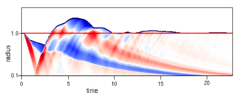
Figure 4: The pressure deviations from the analytic settling solution for a simulation in which a shell with 3 times the ambient density is dropped through the accretion shock. Red (blue) represents pressures higher (lower) than steady-state. The solid horizontal line marks the location of the standing accretion shock at $R=1$. The thin blue curve along the top is the radial trajectory of the perturbed shock. Note the strong reflection of pressure waves at the inner boundary at $t\sim 1.5$. The unit of time in our normalized SAS model corresponds to $\sim 6$ ms in the supernova model shown in Figure 3.

To test the stability of these models, we tried various ways of perturbing the initial solution. In one set of experiments we created a mismatch between the initial conditions and the imposed flow velocity at the inner boundary. If the fixed boundary velocity is set smaller than the flow velocity in the initial analytic solution, the accretion flow is choked off at the inner boundary, and the buildup of pressure initially drives the accretion shock to larger radii. In another set of experiments, we added a large density perturbation in the supersonic free-fall portion of the initial conditions. When this over-dense shell reaches the accretion shock, the increased ram pressure initially drives the shock down to smaller radii.

The results of one of these attempts to perturb the SAS are shown in Figure 4. In all cases the shock front oscillated a few times, but these oscillations were always strongly damped. For the $\gamma=4/3$ solution shown here, the time for material to drift from the accretion shock to the inner boundary is $\tau_{d}=17$, compared to a sound crossing time of $\tau_{s}=1.6$ and a freefall time of $\tau_{f}=0.65$. The shock front rebounds from a perturbation on the relatively short sound-crossing timescale, $\tau_{s}$. For large perturbations this rebound typically overshoots the equilibrium shock radius and subsequent oscillations decay away after several $\tau_{s}$. The accretion shock radius always settled back to within $0.5\%$ of the original steady-state radius after several $\tau_{s}$. The mass accretion rate takes longer to settle down to the steady-state value, as the perturbed postshock flow gradually advects down through the leaky boundary. It is only after a few $\tau_{d}$ that the full effects of the perturbation have advected out of the region and the mass accretion rate at the inner boundary has relaxed to the steady-state value.

These simulations demonstrate that SAS models are stable to radial perturbations. As long as the flow remains spherically symmetric, the accretion shock remains at a fixed radius.

5 INSTABILITY IN TWO DIMENSIONS

To study the stability of standing accretion shocks under the assumption of axisymmetry we ran additional simulations in two dimensions with a variety of initial perturbations, including small density perturbations in the infalling material, weak pressure waves emanating from near the inner boundary, and small random velocity fluctuations in the postshock flow. To quantify the behavior of these accretion simulations our numerical code kept track of several global metrics, including the total kinetic energy (and the component in the angular direction), the thermal and gravitational potential energy of the shocked gas, the total vorticity, the average radius of the accretion shock, and the angular variance in the accretion shock radius.

Figure 5: The growth of interior turbulent energy (defined here as the total kinetic energy in the angular direction) is accompanied by an increase in the average shock radius. The two short-dashed lines correspond to the two-dimensional simulation with spherically symmetric infall, which remains nearly symmetric throughout the evolution. The two solid lines correspond to a two-dimensional simulation initialized with a small asymmetric perturbation. The two long-dashed lines correspond to a similar perturbed model except that the leaky inner boundary has been replaced with a hard reflecting boundary and a thin cooling layer.

All of our two-dimensional SAS simulations proved to be unstable. To illustrate the typical behavior of an axisymmetric accretion shock we will focus on a model with $\gamma=4/3$ and initialized with two rings (a density enhancement of 20%) placed asymmetrically in the preshock flow (see Figure 6). For sufficiently small perturbations, the early evolution is characterized by sound waves bouncing throughout the interior of the accretion shock. These waves are nearly spherically symmetric, but gradually take on an asymmetry characterized by a spherical harmonic with $l=1$. The strength of these asymmetric waves grows with time, and eventually they begin to significantly impact the global properties of the accretion shock. This evolution is shown in Figure 5, where we plot the total energy in angular motion (which we assume to be proportional to the local turbulent energy) and the angle-averaged shock radius. We also show the results for an unperturbed simulation to show that our numerical techniques can hold a SAS stable for at least several dynamical times. From this, we conclude that the introduction of asymmetric perturbations leads to a growing postshock turbulence in standing accretion shocks.

Also shown in Figure 5 is a similar simulation but with different inner boundary conditions: a reflecting wall plus a thin cooling layer. The initial radial solution is nearly identical to the adiabatic solution except close to the inner boundary, where the cooling becomes strong and the gas quickly settles into a thin layer on top of the hard surface. As shown in Figure 5, the evolution is qualitatively the same as in the adiabatic model with a leaky boundary. This comparison verifies the independence of these results from the details of the boundary conditions.

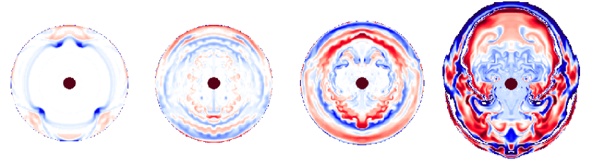
Figure 6: Images of the gas entropy (red is higher than the equilibrium value, blue is lower) illustrate the instability of a spherical standing accretion shock. This model has $\gamma=4/3$ and is perturbed by placing over-dense rings into the infalling preshock gas. Note that with the scaling for a realistic supernova model, the last image on the right corresponds to $\sim 300$ ms. These simulations are axisymmetric, forcing a reflection symmetry about the vertical axis.

To further illustrate this early evolution we show a time series of the two-dimensional flow in Figure 6. We use the gas entropy to visualize the flow because a steady, spherical shock would produce a postshock region of constant entropy. Thus, any deviation from a spherical shock shows up as a change in the postshock entropy. Aside from the overall trend of growing perturbations in the postshock entropy, this figure illustrates the dominance of low-order modes. This is a generic result of our two-dimensional simulations. While the wave modes in the early evolution depend on the initial perturbations, the $l$ = 1 mode always grows to dominate the dynamics.

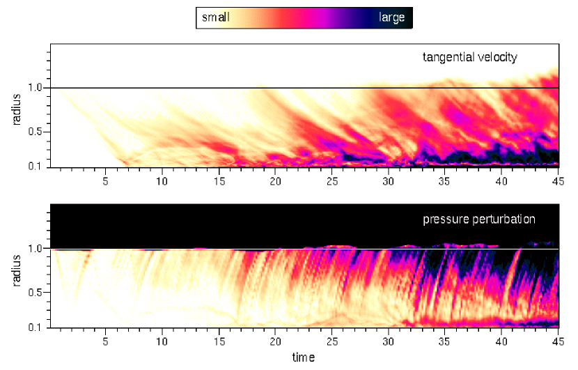
Figure 7: The time evolution of a 2D simulation is illustrated in spacetime diagrams. The color at a given radius and time corresponds to the angle-average of the absolute value of the tangential velocity (top) and absolute value of the deviation of pressure from the steady-state solution, $\Delta P/P$ (bottom). Regions that are under-pressured with respect to the steady-state solution collect near the bottom of the “atmosphere” after $t\sim 15$ and correspond to the centers of strong vorticies that have become trapped at these radii by advection. Direct evidence of these vortices are seen in the velocity plot.

To better understand the origin of the SAS instability we show a spacetime diagram of angle-averaged quantities in Figure 7. Here we see two dominant trends: (1) pressure waves rising up from small radii at the local speed of sound to perturb the shock front and (2) regions of high transverse velocity originating at the shock and advecting downwards at the local flow speed (slower than the sound speed). It is the feedback between these two waves (at least for low values of $l$) that leads to amplification of the initial perturbations. Aspherical pressure waves rising up to the accretion shock distort the shock front from its equilibrium spherical shape. The slight obliquity of the shock front relative to the radial pre-shock flow then creates non-radial post-shock flow that advects inward, feeding turbulent flow at small radii. This growing turbulence in turn drives stronger aspherical pressure waves that propagate upwards and further distort the accretion shock. This feedback was discovered independently in the context of accretion onto a black hole by Foglizzo (2002), who dubbed it a “vortical-acoustic” cycle.

To contrast this with planar flow, any vorticity generated by perturbations to the planar shock front are advected downstream, unable to impact the shock dynamics. In the case of an SAS, however, the vorticity is trapped in a finite volume. With nowhere to go, the vorticity grows with time and eventually becomes strong enough to affect the shock front.

Figure 8: The change in energy ($E-E_{o}$) of the postshock gas is shown for the total (solid), kinetic (long dash), thermal (short dash), and gravitational potential (dotted) energies. The initial values, $E_{o}$, are -15.8, +0.08, +47.6, and -63.5, respectively.

Once the turbulent energy density in the postshock flow becomes significant, the volume of the shocked gas begins to grow with no apparent bound. The origin of this increase in shock radius can be traced to the distribution (kinetic versus thermal versus gravitational) of total energy below the shock. Note that this is strictly adiabatic flow—there is no source of external heating to assist in driving the shock outwards. The total energy on the computational grid remains relatively constant (the total energy of the gas flowing off the inner edge of the grid is small and varies slightly due to the growing turbulence, while the total energy of the gas falling onto the grid from the outer boundary is approximately zero), but the distribution of energy changes. As the nominally spherical accretion shock becomes more distorted, the postshock gas retains more kinetic energy at the expense of thermal energy. This gradual change can be seen in a plot of the various components of the total energy (the three terms in eqn. 9) integrated over the volume of shocked gas. This is shown in Figure 8. Moreover, this redistribution of energy among kinetic, thermal, and gravitational components results in a redistribution of the total energy per unit mass in the postshock gas. In Figure 9 we see that, as the instability described here develops, an increasing fraction of the postshock gas attains positive energies at the expense of gas that becomes more bound. There is no new source of energy in this system, only a redistribution of energy.

Figure 9: We plot the mass fraction of postshock gas with total energy per unit mass (scaled to the local gravitational potential energy) above a given value, $E$. In the initial SAS solution, all of the postshock gas has a total scaled energy per unit mass of $E=-0.245$ for $\gamma=4/3$; therefore, the sequence shown in this figure begins as a step function at that value. With time, the gas becomes redistributed in energy, with some gas having more negative total energy and some gas having substantially more positive total energy. At late times, a significant fraction of the postshock gas has $E>0$.

To follow the long-term evolution of an SAS we continued the simulation of our standard model, with $\gamma=4/3$, but allowed the numerical grid to expand radially to accommodate the increasing shock radius. We followed the expansion out to a radius of 15 in this fashion. The evolution can be broken into three distinct epochs. At early times ($t<40$) the shock remains roughly spherical, and the volume of shocked gas is approximately constant while the interior turbulent energy grows steadily. The intermediate epoch is characterized by large oscillations in the postshock flow that lead to an aspect ratio for the accretion shock that varies between one and two. The volume of shocked gas exhibits a growing oscillation, reminiscent of a breathing mode. This phase of the evolution is dominated by the $l$ = 1 mode; i.e., is distinctly oscillatory. Beyond a time of 170, the flow takes on a strikingly self-similar form dominated by the $l$ = 2 mode; i.e., is distinctly bipolar. The aspect ratio becomes remarkably constant at a value $\sim 2$ (2.3 to be precise), but the scale of this aspherical shock grows roughly linearly with time. From $t=165$ to $t=225$, the angle-averaged shock radius increases from 5 to 15. This corresponds to an expansion velocity of order 50% the escape velocity at the shock. This self-similar expansion is illustrated in Figure 10, where we plot images of the gas entropy at three different times chosen such that the shock has roughly doubled in size in each interval. When scaled to the same size, the images look qualitatively similar.

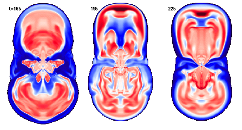
Figure 10: The self-similar growth of the asymmetric accretion shock is illustrated in these entropy images from three different times in our simulation. The postshock volume grows with time, but each successive image is scaled down by a factor of two to produce three images of roughly the same size. Here blue (red) represents low (high) entropy.

The dynamics of this self-similar state are illustrated in Figure 11. The global features include a dominant accretion flow in the equatorial region and mildly supersonic, quasi-periodic outflows along the two poles. These outflows are fed by accreting gas that “misses the target.” The oblique shocks near the equator lead to low-entropy gas advecting in (as material hits the shock at an increasingly oblique angle, it does not suffer as large a change in entropy when traversing the shock).

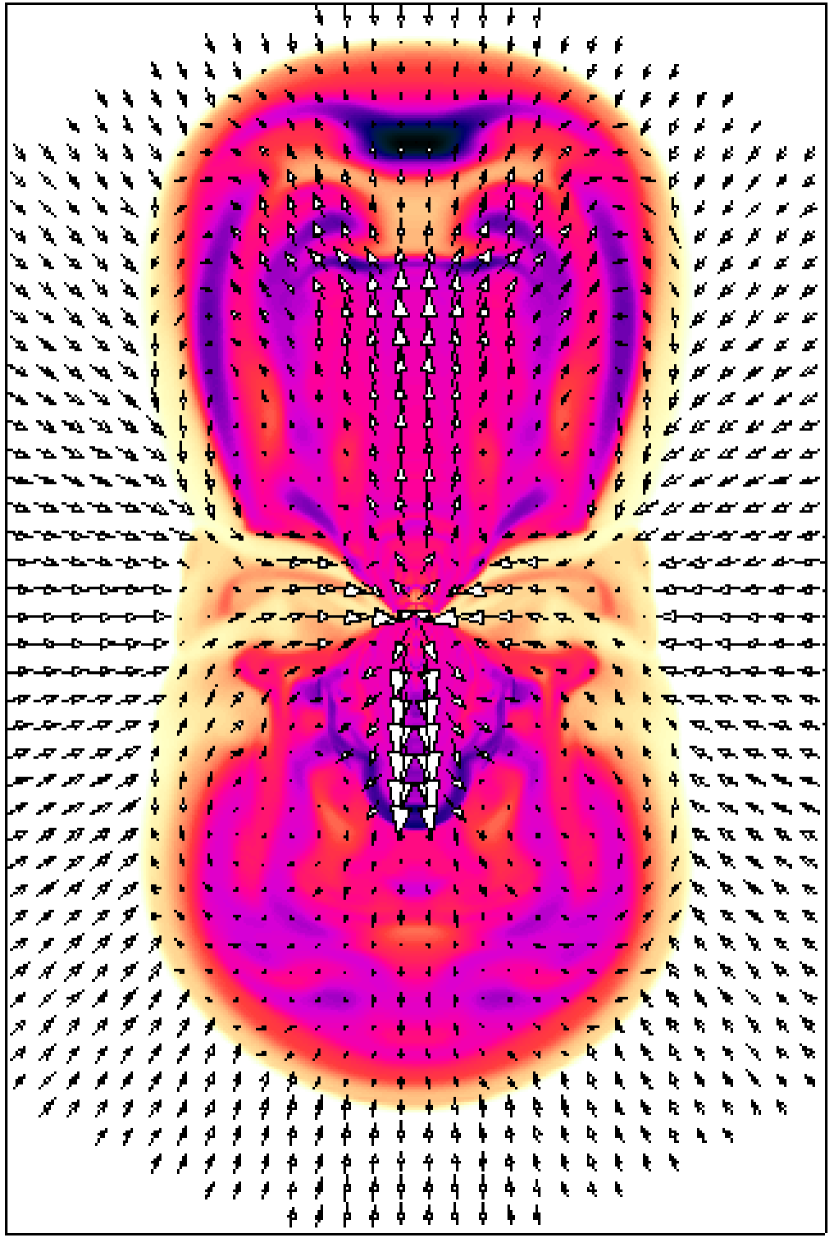
Figure 11: The expansion of the accretion shock is driven by accretion in the equatorial plane feeding quasi-periodic outflows along the symmetry axis. The color scale in this image depicts gas entropy, with dark colors representing high entropy.

The only two parameters in this idealized SAS model are the adiabatic index, $\gamma$, and the radius of the inner boundary, $R_{i}$. We ran several simulations varying these parameters and found qualitatively similar results in virtually all the simulations, but with two clear trends, illustrated in Figure 12. Simulations with a larger value of $R_{i}$, and hence less volume for postshock turbulence to develop, exhibited a slower growth in the total turbulent energy. Herant, Benz, & Colgate (1992) pointed out that the scale of convection in a confined spherical shell scales with the ratio of the inner to the outer boundaries. By analogy we might then expect the dominant mode of instability in the accretion shock to scale with $R_{i}$: the larger the value of $R_{i}$, the larger the value of $l$ of the dominant mode. While the growth of the instability was slower, all of our models did eventually evolve into a strong bipolar mode that drove the shock out to larger radii. Even the simulation with $R_{i}=0.4$ rapidly grew to a turbulent energy of 0.6 by a time of 80. We also found slower growth of the SAS instability with smaller values of $\gamma$. Only in the case of a very soft equation of state ($\gamma=1.25$) did the shock remain marginally stable for several flow times. Eventually, this model became as unstable as the others, with a growing bipolar accretion shock. While all of the SAS models are unstable, a decrease in the effective adiabatic index and spatial extent of the postshock flow does appear to slow the growth of the instability. Note that both of these trends might work against the growth of the instability in the evolution of core-collapse supernovae, where the effective adiabatic index is lower and the postshock volume is affected by neutrino cooling.

Figure 12: The dependence of the SAS instability on the model parameters is shown here by looking at the growth of the interior turbulent energy for several different simulations corresponding to different inner boundary radii (left graph: from top to bottom, $R_{i}$ = 0.05, 0.1, 0.2, and 0.4) and different adiabatic indices (right graph: from top to bottom $\gamma$= 1.4, 1.33, and 1.25, with $R_{i}$ fixed at 0.1).

6 CONCLUSION AND DISCUSSION

Our primary conclusion is that relatively small-amplitude perturbations, whether they originate from inhomogeneities in the infalling gas, aspherical pressure waves from the interior region, or perturbations in the postshock velocity field can excite perturbations in a standing accretion shock that lead to vigorous turbulence and large-amplitude variations in the shape and position of the shock front.

It is important to note that this behavior is not driven by convection: the initial conditions in our SAS model are marginally stable to convection. Furthermore, during the course of our simulations the angle-averaged entropy remains relatively constant with radius. In Figure 6 we can see the development of convection on small scales from local entropy gradients in the flow below the accretion shock. However, there is no global gradient extending over the entire postshock region, driving convection on that scale.

Our models clearly show an evolution to low-order modes, as first seen in the early two-dimensional supernova models of Herant, Benz, & Colgate (1992). Independent of the initial seed, our models were eventually dominated by either an $l=1$ or $l=2$ mode after several flow times; these were the only modes that ever became highly nonlinear. Moreover, once these low-order modes began to dominate, the average shock radius began to grow, altering the global behavior from a standing accretion shock to an expanding aspherical blastwave.

Our work also suggests that large-scale ($l$ = 1 or 2) modes may dominate the late-time evolution of core-collapse supernovae, although our models cannot directly address this possibility because the assumption of supersonic freefall above the shock is no longer valid once the shock encounters the subsonic regions in the stellar core. Nonetheless, it is interesting to note that when our outflows become self similar, they achieve an aspect ratio $\sim 2$. This is within the range suggested by spectropolarimetry data (e.g., Höflich, Khokhlov, & Wang, 2001). Could it be that the polarization uniformly observed in core collapse supernovae is a signature of the unstable growth of $l=1,2$ modes in the initial explosion? Moreover, if the SAS instability is responsible for generating the large aspect ratios in observed explosions, it provides at least one example where a “conventional” neutrino-driven explosion model can be constructed that is not in conflict with these observations, a concern expressed by Wang et al. (2001).

While our results are relatively independent of the initial conditions, we note that the amplitude and scale of our seed perturbations are consistent with those expected to be produced by the late stages of shell burning in presupernova stars (Bazan & Arnett, 1998) or in the core collapse process itself. Bazan and Arnett followed the evolution of shell oxygen burning in a presupernova star and found that unstable nuclear burning can lead to significant density perturbations. When this layer of the progenitor star falls through the accretion shock, it can excite the instabilities found here. Alternatively, entropy-driven postshock convection (Herant et al., 1994; Burrows, Hayes, & Fryxell, 1995; Janka & Mueller, 1996; Mezzacappa et al., 1998; Fryer & Heger, 2000) could provide the necessary seeds for this shock instability. Yet another possibility is the growth of lepton-driven convection (Keil, Janka, and Mueller, 1996) or neutron fingers (Wilson & Mayle, 1993) deep in the proto-neutron star. If these grow to sufficient amplitude, they would drive aspherical pressure waves out into the accreting postshock gas, exciting this shock instability.

This instability exists! We have used time-dependent hydrodynamic simulations to show that a simple adiabatic model of a standing accretion shock that is stable in one dimension is unstable in two dimensions. The physical mechanism responsible for this instability appears to be the feedback between aspherical-shock–induced vorticity and the pressure waves generated by this vorticity. This feedback was also discovered in the context of accreting black holes and dubbed a “vortical-acoustic” feedback by Foglizzo (2002). We note that Houck & Chevalier (1992) performed a linear stability analysis of steady, spherical accretion flows with cooling. We have used one of these models to test the effect of different inner radial boundary conditions on our simulation outcomes. For $\gamma=4/3$, our one-dimensional simulations are in agreement with their results. In particular, we find that the shock is stable for small values of the shock stand-off distance (when the shock is less than 20 times the radius of the inner boundary surface) and unstable for larger values. However, for $\gamma=4/3$ Houck & Chevalier (1992) did not extend their analysis to the nonradial case; therefore, we cannot directly compare their results with our findings in this case.

Many questions must be answered before we can determine whether this vortical-acoustic instability plays an important role in core-collapse supernovae. Will neutrino cooling near the proto-neutron star surface dampen the feedback mechanism by damping the pressure waves? Will neutrino cooling below the shock drive the flow away from conditions under which an instability can develop by reducing the postshock volume? In the models considered here, radiative losses were neglected, although mimicked in one case by using a soft ($\gamma=1.25$) equation of state. In this case the instability was weakened but still developed into an aspherical flow.

Neutrino cooling and heating will have several important consequences for the development of the instability described here: (1) As mentioned above, neutrino cooling may affect the generation of pressure waves at the base of the density cliff associated with the surface of the proto-neutron star. (2) Neutrino cooling and heating will, in part, determine the postshock volume between the density cliff and the supernova shock, which in turn will, in part, determine which $l$ modes may grow in the postshock flow. (3) Neutrino heating may selectively drive modes other than the fastest growing, $l=1,2$, modes. Moreover, the effects due to neutrino cooling and heating will be time dependent. Once an explosion is underway, the cooling region will be confined to the surface of the proto-neutron star, although pressure waves may still be damped, and the heating region will increase in volume, allowing lower-$l$ modes to develop—perhaps the $l=1,2$ modes.

One can already begin to assess the relevance of the SAS instability to the core-collapse supernova problem by comparing our models with previous multidimensional core-collapse supernova models. In Mezzacappa et al. (1998), once the shock front is distorted by the initial neutrino-driven convection, the SAS instability does appear to affect the postshock flow a few hundred ms after bounce. The shock front is significantly distorted from the initial spherical shape, and this oblique shock feeds strong interior turbulence. However, unlike in our SAS models, the $l=1$ mode in fact did not come to dominate the postshock flow. Rather, $l\sim$few modes dominated at the shock’s peak radius and later were “squeezed out” as the shock receded. In this case, owing to neutrino cooling and the lack of sufficient neutrino heating, the separation between the shock front and the surface of the proto-neutron star was never sufficient for low-$l$ modes of the SAS instability to develop. To test this hypothesis we ran a two-dimensional SAS model with an inner boundary at 0.6, comparable to the effective surface of the proto-neutron star relative to the shock front at late times in the simulations of Mezzacappa et al. (1998). While low-$l$ modes did exist, they were unable to grow significantly in such a confined geometry. This dependence on the shock radius with respect to the surface of the proto-neutron star further emphasizes the need for realistic neutrino heating and cooling—i.e., neutrino transport—in multidimensional supernova models.

The simulations of Burrows, Hayes, & Fryxell (1995) clearly exhibit strong turbulence fed by an aspherical shock at late times. However, they included only one quadrant in their explosion simulation, and, therefore, neither an $l$ = 1 or 2 mode was allowed. In the simulations described in Janka & Mueller (1996), one can again identify a close link between the deformed accretion shock and strong large-scale vorticies in the postshock flow. Furthermore, by the end of their simulations, at $\sim 700$ ms, it appears that the $l=1$ mode is beginning to dominate. An interpretation of the SPH models of Herant et al. (1994) in our context is complicated by the fact that their simulation is also confined to a $90^{o}$ wedge, cutting off the lowest order modes. Furthermore, their explosion time scale is relatively short, providing insufficient time for the long wavelength SAS instability to develop. This short explosion timescale is most likely the result of their neutrino transport implementation.

It is interesting to note that the instability we identify in this paper may provide a somewhat revised paradigm for powering core collapse supernovae. In the models we presented here, explosions were obtained in the absence of neutrinos, powered by gravitational binding energy. The SAS instability serves to redistribute the energy of the flow into kinetic energy at the expense of internal and gravitational energy. Thus, both the instability and neutrinos may serve as vehicles to convert gravitational binding energy into the kinetic energy of explosion. If the SAS instability does in fact play a role in the explosion mechanism in more realistic models, it would be interesting to compute, if possible, the contributions to the kinetic energy in the explosion that result from these two vehicles. Moreover, it has been pointed out that the energies of explosions powered by neutrino heating may be limited to $1-3\times 10^{51}$ erg (Janka, 2001). If the SAS instability sets in and also serves to power the supernova, we may end up with a more energetic explosion, one only partially powered by neutrinos. On another front, it is interesting to note that the SAS instability may help alleviate the precarious balance that is struck during neutrino shock reheating—between accretion luminosity, mass accumulation in the gain region, and ram pressure. As pointed out by Janka (2001), it is necessary to maintain sufficient neutrino luminosity and mass in the gain region to power an explosion, and this is achieved by maintaining a sufficient level of mass accretion through the shock and onto the proto-neutron star. On the other hand, this accretion is the source of the ram pressure the shock combats in its attempt to propagate outward in the stellar core. If neutrino heating is able to sustain a sufficiently large shock radius for a period of time, the SAS instability may act to initiate the explosion, removing some of the burden from the neutrinos.

There are other factors that may influence the role of shock instability in core-collapse supernovae. How will rotation and/or magnetic fields couple to this mechanism? For example, will rotation provide sufficient distortion of the accretion shock to help drive low-$l$ modes? And will this lead to an explosion where otherwise (in the absence of rotation) one would not occur? It may be that a combination of near-explosive conditions and rotation will be required before the instability we describe can develop. If it does, it will certainly contribute to the explosion and should be considered an ingredient in the explosion mechanism.

Our results are certainly influenced by the imposed axisymmetry of our two-dimensional simulations. For example, our bipolar outflows may be an artifact of our boundary conditions, although the aspect ratio we observe when our flows become self similar is certainly an independent feature; we could have obtained bipolar outflows with very different aspect ratios. Generally speaking, will the SAS instability exist in three dimensions? Will the low-order modes still dominate the flow? Will rotation serve the role in three dimensions that the imposed axisymmetry serves in two? Three-dimensional simulations are underway, and we hope to report on them soon.

References

- Bazan & Arnett (1998) Bazan, G. & Arnett, W. D. 1998, ApJ, 496, 316
- Burrows, Hayes, & Fryxell (1995) Burrows, A., Hayes, J., & Fryxell, B. A. 1995, ApJ, 450, 830
- Chevalier (1989) Chevalier, R. A. 1989, ApJ, 346, 847
- Colella & Woodward (1984) Colella, P., & Woodward, P. R. 1984, JCP, 54, 174
- Foglizzo (2002) Foglizzo, T. 2002, A&A, 392, 353
- Fryer & Heger (2000) Fryer, C. L. & Heger, A. 2000, ApJ, 541, 1033
- Herant, Benz, & Colgate (1992) Herant, M., Benz, W., & Colgate, S. A. 1992, ApJ, 395, 642
- Herant et al. (1994) Herant, M., Benz, W., Hix, W. R., Fryer, C. L., & Colgate, S. A. 1994, ApJ, 435, 339
- Höflich, Khokhlov, & Wang (2001) Höflich, P., Khokhlov, A., & Wang, L. 2001, in Proc. of 20th Texas Symposium on Relativistic Astrophysics, eds. Wheeler, J. C. & Martel, H. (New York: American Institute of Physics)
- Houck & Chevalier (1992) Houck, J. C. & Chevalier, R. A. 1992, ApJ, 395, 592
- Janka (2001) Janka, H.-T. 2001, A&A, 368, 527
- Janka & Mueller (1996) Janka, H.-T. & Müller, E. 1996, A&A, 306, 167
- Keil, Janka, and Mueller (1996) Keil, W., Janka, H.-T., & Müller 1996, E., ApJL, 473, L111
- Leveque (1998) LeVeque, R. J. 1998, in 27th Saas-Fee Advanced Course Lecture Notes, eds. Steiner, O. & Gautschy, A. (New York:Springer-Verlag)
- Mezzacappa et al. (1998) Mezzacappa, A., Calder, A. C., Bruenn, S. W., Blondin, J. M., Guidry, M. W., Strayer, M. R., & Umar, A. S. 1998, ApJ, 495, 911
- Mezzacappa et al. (2001) Mezzacappa, A., Liebend rfer, M., Messer, O. E. B., Hix, W. R., Thielemann, F.-K., & Bruenn, S. W. 2001, PRL, 86, 1935.
- Wang et al. (2001) Wang, L., Howell, D. A., Höflich, P., & Wheeler, J. C. 2002, ApJ, 550, 1030
- Wilson & Mayle (1993) Wilson, J. R. & Mayle, R. 1993, Physics Reports 227, 97
- Whitham (1974) Whitham, G. B. 1974, Linear and Nonlinear Waves (New York: John Wiley and Sons)