An Optical Bow Shock Around the Nearby Millisecond Pulsar J2124–3358

Abstract

We report the discovery of an H$\alpha$-emitting bow-shock nebula powered by the nearby millisecond pulsar J2124–3358. The bow shock is very broad, and is highly asymmetric about the pulsar’s velocity vector. This shape is not consistent with that expected for the case of an isotropic wind interacting with a homogeneous ambient medium. Models which invoke an anisotropy in the pulsar wind, a bulk flow of the surrounding gas, or a density gradient in the ambient medium either perpendicular or parallel to the pulsar’s direction of motion also fail to reproduce the observed morphology. However, we find an ensemble of good fits to the nebular morphology when we consider a combination of these effects. In all such cases, we find that the pulsar is propagating through an ambient medium of mean density $0.8-1.3$ cm^-3 and bulk flow velocity $\sim 15-25$ km s^-1, and that the star has recently encountered an increase in density by $1-10$ cm^-3 over a scale $\lesssim 0.02$ pc. The wide variety of models which fit the data demonstrate that in general there is no unique set of parameters which can be inferred from the morphology of a bow-shock nebula.

1. Introduction

Many pulsars experience significant ram pressure as they move through the interstellar medium (ISM). This pressure can confine the pulsar’s relativistic wind and generate a bow-shock pulsar wind nebula (PWN). The H$\alpha$ emission generated by such sources provides an important probe of the pulsar’s interaction with its environment (see Chatterjee & Cordes (2002) for a recent review). However, until recently only three H$\alpha$ PWNe were known, and we consequently have lacked a detailed understanding of this phenomenon.

We are carrying out a survey for new pulsar bow shocks in the southern sky. We have previously reported the discovery of a faint H$\alpha$ PWN surrounding PSR B0740–28 (Jones, Stappers, & Gaensler (2002)). We here present another new H$\alpha$ pulsar bow shock, associated with the nearby millisecond pulsar J2124–3358 (Bailes et al. (1997)). A recent timing ephemeris (M. Bailes, private communication) yields a spin period of 4.93 ms and a position (at MJD 50288.0) of RA (J2000) $21^{\rm h}24^{\rm m}43\fs 86196(6)$, Dec. (J2000) $-33^{\circ}58^{\prime}44\farcs 257(1)$, where the numbers in parentheses indicate the uncertainty in the last digit. The pulsar’s intrinsic spin-down luminosity is $\dot{E}=4.3\times 10^{33}$ erg s^-1 (Toscano et al. (1999)), while its dispersion measure of 4.61 pc cm^-3 implies a distance of $270\pm 20$ pc (Cordes & Lazio (2002)). In future discussion, we adopt a distance $D=270d_{0}$ pc to the source.

The pulsar timing ephemeris yields a proper motion relative to the solar system barycenter of $52.6(3)$ milliarcsec yr^-1 at position angle $195\fdg 6(3)$ (North through East). Because of the pulsar’s proximity and low space velocity, the peculiar motion of the sun with respect to the Local Standard of Rest needs to be accounted for. In the case of PSR J2124–3358, the sun’s motion is directed almost perpendicular to the line-of-sight, and so contributes a significant component of the observed proper motion. After correction for the solar peculiar velocity (and for the small effects of differential Galactic rotation), we find that the motion of the pulsar relative to its local standard of rest is 47(3) milliarcsec yr^-1 at position angle $209(3)^{\circ}$, corresponding to a projected space velocity of $(61\pm 4)d_{0}$ km s^-1. The uncertainties in the direction and magnitude of the solar motion dominate those in the pulsar’s distance and measured proper motion.

2. Observations and Results

The field around PSR J2124–3358 was observed for 4800 sec on 2001 July 25 (MJD 52115) with a narrowband H$\alpha$ filter on the 3.5-m New Technology Telescope (NTT) at the European Southern Observatory, La Silla, Chile. The mean seeing was $\sim 1\farcs 2$; all other observational parameters were as described by Jones et al.  (2002). Standard techniques for bias and flat-field correction were used to remove instrumental signatures from the data. Individual frames were dithered to permit removal of CCD defects and cosmic rays using median filtering on the frames when combined. An astrometric solution was determined using 10 field stars with positions in the USNO Catalog. The iraf task ccmap was used to fit the positions with a third order polynomial with cross terms. The RMS scatter was $(\Delta\alpha,\Delta\delta)$ = ($\pm 0\farcs 15$,$\pm 0\farcs 07$) and the residuals uniformly scattered. A transformation of the derived USNO star coordinates back onto the image did not reveal any systematic offsets between the observed and derived positions.

Figure 1 shows a smoothed H$\alpha$ image of the field surrounding PSR J2124–3358. The position of the pulsar at epoch MJD 52115 is marked, as is the pulsar’s direction of motion with respect to its local standard of rest. The pulsar is located just inside the apex of an optical nebula with a clear bow-shock morphology, while the pulsar’s projected velocity points within $\sim 30^{\circ}$ of the apparent nebular symmetry axis. This confirms that the nebula is a bow-shock PWN powered by the pulsar.

The morphology of this PWN deviates in several ways from the classic bow-shock shape predicted by theory. The eastern half of the nebula is dominated by a marked kink (indicated with a “K” in Figure 1), located about $25^{\prime\prime}$ north-east of the pulsar. North of this kink the opening angle of the bow shock becomes significantly broader; this eastern limb of the nebula fades into the background $\approx 1\hbox{$.\!\!^{\prime}$}5$ from the pulsar. The western half of the nebula is generally more uniform in its shape and brightness than the eastern half. On the western side, the opening angle of the bow shock reaches a maximum $\sim 1^{\prime}$ from the pulsar, before starting to closing back in on itself. This half of the nebula extends $\sim 2^{\prime}$ from the pulsar.

H$\alpha$ emission from the head of the nebula is clearly resolved, with a thickness adjacent to the pulsar of $3^{\prime\prime}$, decreasing to $2^{\prime\prime}$ in parts of the nebula to the pulsar’s north-east and north-west. The head of the PWN is highly asymmetric around the pulsar’s velocity vector, being considerably broader to the west of this axis than to the east.

The H$\alpha$ flux density was calculated from an unsmoothed frame in the manner described by Jones et al.  (2002), using the planetary nebula G321.3–16.7 as a flux standard. Considering an $8^{\prime\prime}$-wide curved strip enclosing the entire visible nebula, we find that the H$\alpha$ flux for the PWN powered by PSR J2124–3358 is $2.5\times 10^{-4}$ photons s^-1 cm^-2. The mean surface brightness is $7.4\times 10^{-19}$ erg s^-1 cm^-2 arcsec^-2, three times that measured for PSR B0740–28 (Jones et al.  2002) or one-tenth of that for PSR J0437–4715 (Bell et al. (1995)). Both in the immediate vicinity of the pulsar and at the kink, the nebula’s surface brightness is $1.5\times 10^{-18}$ erg s^-1 cm^-2 arcsec^-2, a factor of $\sim 2$ brighter than the nebular average.

3. Discussion

The position, speed and direction of motion of PSR J2124–3358 have all been determined to reasonably high precision (see §1). This system thus presents an excellent opportunity to model a bow-shock PWN and to constrain its parameters.

To quantify the properties of this nebula, we consider a pulsar of space velocity $V$ moving through an ambient medium of mass density $\rho_{0}$ and number density $n_{0}$. We define the “stand-off distance”, $R_{0}$, to be the characteristic scale size of the nebula. For an idealized bow shock, $R_{0}$ is the distance from the pulsar to the apex of the bow shock along the direction of motion. The corresponding “stand-off angle” is $\theta_{0}=R_{0}\sin i/D$, where $i$ is the inclination of the pulsar’s motion to the line-of-sight (see Equation [4] of Chatterjee & Cordes (2002)). We further define the “bow-shock angle”, $\psi_{0}$, to be the angular separation between the pulsar and the outermost edge of the projected H$\alpha$ emission along the projected direction of the pulsar’s motion. In general, $\psi_{0}$ is the only parameter which can be directly measured from an image; in this case $\psi_{0}\approx 2\farcs 6$.

We crudely estimate the parameters of the system by assuming that $i=90^{\circ}$, and that the outer edge of the observed H$\alpha$ emission demarcates the bow shock structure. In this case $\theta_{0}\equiv\psi_{0}$ and so $R_{0}\approx 0.003d_{0}$ pc. At the stand-off distance, pressure from the pulsar wind, $P_{\rm PSR}=\dot{E}/4\pi R_{0}^{2}c$, balances the ram pressure of the ambient medium, $P_{\rm ISM}=\rho_{0}V^{2}$, so that $n_{0}=1.6d_{0}^{-4}$ cm^-3. This confirms that the pulsar is embedded in the warm, neutral component of the ISM (e.g. Kulkarni & Heiles (1988)), as expected for observable H$\alpha$ bow shocks. The corresponding ISM sound speed is $c_{s}\sim 5$ km s^-1, and the Mach number for the pulsar is $M=V/c_{s}\gtrsim 12$.

We now consider the detailed morphology of the head of the nebula. We first rotate the image counterclockwise by $61^{\circ}$, so that the pulsar’s motion is strictly from left to right, and adopt an $(x,y)$ coordinate system with the pulsar at the origin. We then by hand identify a series of points which demarcate the outermost boundary of the head of the optical nebula, over an azimuthal range of $\sim 120^{\circ}$ on either side of the pulsar’s direction of motion. The resulting data-points can then be fit with a variety of functional forms. We note that variations in thickness and brightness seen in the nebula potentially provide additional information on the pulsar’s interaction with its environment. However, to use these data, one must take into account the width and surface density of the emitting regions as a function of position, and also must consider the effects of charge-exchange and collisional excitation (Bucciantini & Bandiera (2001); Bucciantini 2002b ). Given these considerable complications, here we consider only the overall shape of the emitting regions, as delineated by the outermost edge of the H$\alpha$ nebula.

We first consider the idealized case of an isotropic wind propagating through a homogeneous ambient medium. In this case, the shape of the bow-shock surface is given by (Wilkin (1996)):

$$R(\phi)=\kappa R_{0}/\sin\phi\sqrt{3(1-\phi/\tan\phi)},$$ (1)

where $R(\phi)$ is the distance from the pulsar to a given point on the bow-shock surface, $\phi$ is the angle between the velocity vector and the vector joining the pulsar to this point, and $\kappa$ is a constant, with value $\kappa=1$ in this case.

In panels A and B of Figure 2, we show solutions to Equation (1) for $i=90^{\circ}$ and $i=30^{\circ}$ respectively, scaled to match the data so that for $\phi=0^{\circ}$, the angular separation between the pulsar and the outermost edge of the bow-shock surface is $\psi_{0}\approx 2\farcs 6$. Best-fit parameters for each solution are listed in Table 1. (As an aside, we note that unless $i=90^{\circ}$, the usual assumption that $\theta_{0}\equiv\psi_{0}$ is incorrect. For example, for the inclined case $i=30^{\circ}$ we find that $\theta_{0}=\kappa R_{0}\sin i/D=0\farcs 8\ll\psi_{0}$. This indicates that in cases where the inclination angle is not known, the first-order assumption that $\theta_{0}=\psi_{0}=\kappa R_{0}/D$ results in an upper limit on $\kappa R_{0}$ and a lower limit on $n_{0}$, in contrast to previous calculations [see e.g. §5.1 of Chatterjee & Cordes (2002)].)

These plots make clear that for any inclination, the observed nebula is too broad and too asymmetric to be described by Equation (1). However, in comparing a pulsar bow shock to the shape described by Equation (1), a number of caveats must be made. First, Equation (1) describes a system in which radiative cooling is efficient, and in which there is significant mixing between the stellar wind and ambient material (Wilkin (1996)), neither of which is likely to be the case for pulsar bow shocks (Bucciantini & Bandiera (2001)). However, these effects do not change the shape of the bow shock, but simply require $\kappa\sim 1.7-2.4$ in Equation (1) (Bucciantini 2002a ; van der Swaluw et al. (2002)). van der Swaluw et al.  (2002) also demonstrate that for low Mach numbers $M\lesssim 5$, the tail of the resulting bow shock is slightly broader than that described by Equation (1). However, in this case we have demonstrated above that $M>12$, sufficiently high that a morphology close to the analytic shape should result.

We are thus forced to conclude that the idealized bow-shock morphology is unable to describe this nebula. To account for the observed appearance, we must relax some of the assumptions from which Equation (1) was derived. Specifically, we need to consider the possibilities of a density gradient in the ISM, a significant flow velocity for the ambient medium, or of anisotropies in the pulsar wind. We briefly summarize how each of these effects manifest themselves in the observed nebular morphology:

1. A local density gradient perpendicular to the pulsar’s direction of motion will distort the bow-shock shape of Equation (1) so that the head of the nebula is narrower on the side where the density is higher, and broader on the side where the density is lower. We here consider a nebula in an exponential density gradient of e-folding scale $\kappa lR_{0}$, using the analytic solution provided by Wilkin (2000).

2. A density gradient parallel to the pulsar velocity vector results in a time-variable ambient gas pressure. The stand-off distance will thus continually change to adjust for this pressure imbalance, decoupling the position of the pulsar from that of its bow-shock. A detailed treatment of this process is beyond the scope of this paper; here we approximate the effects of such a gradient by using Equation (1), but with the nebula shifted along the $x$-axis by an amount $-R_{1}$. This crudely corresponds to an increase in ambient density by a factor $\sim(\kappa R_{0})^{2}/(\kappa R_{0}-R_{1})^{2}$ over a length scale $\sim\kappa R_{0}$. If we assume an exponential density gradient with e-folding scale $\kappa mR_{0}$, we then find that $m\sim-1/[2\ln(1-R_{1}/\kappa R_{0})]$. Note that this approximate treatment only describes the behavior in the narrow region between the pulsar and the apex of the bow shock; we assume here that the pulsar has only recently encountered the density gradient, so that the overall nebular morphology has the form of Equation (1) with constant $R_{0}$.

3. Bulk motion of the ambient gas (in the reference frame of Galactic rotation at that position) will result in a nebula as described by Equation (1), but with the nebula rotated by some angle $\omega$ about the pulsar position. The angle $\omega$ is determined by subtraction of the ISM flow velocity vector from the pulsar velocity vector.

4. An anisotropic wind can generate a wide variety of complicated bow-shock morphologies, depending on the geometry and orientation of the outflow (Bandiera (1993); Wilkin (2000)). Wilkin (2000) derives analytic solutions for the bow shocks generated by axisymmetric winds, parameterizing the resulting morphologies via the variable $c_{2}$ and $\lambda$. The parameter $c_{2}$ indicates the nature of the wind (see Equation [109] of Wilkin (2000)): $c_{2}=3$ corresponds to a completely polar wind, $c_{2}=0$ to an isotropic wind, and $c_{2}=-1.5$ to a completely equatorial wind. The parameter $\lambda$ is the angle between the pulsar spin axis and the pulsar velocity vector.

We have generated an exhaustive set of bow-shock morphologies corresponding to each of the above four models, for all reasonable free parameters and for all inclination angles. For each of these models alone, we are unable to find a set of parameters which can match the observed bow-shock morphology: a perpendicular density gradient or ISM bulk flow can generate a nebula which is asymmetric about the $x$-axis (as seen in panels C and D of Figure 2) but which is too narrow to match the data, while a a parallel gradient or anisotropic wind can generate a broader bow shock (as seen in panels E and F of Figure 2) but cannot account for the high level of asymmetry between the top and bottom halves of the nebula.

However, when we combine two or more of these effects, we find that we can match the morphology of the head of the nebula with a wide variety of parameters. A representative selection of such fits are listed in the lower half of Table 1; in all cases, the predicted bow-shock morphology corresponds well to that of the H$\alpha$-emitting nebula. We plot three of these models in Figure 2: in model H, there is a density gradient at an angle to the pulsar’s motion (in this case at an approximate PA of $225^{\circ}$ in Figure 2) and a bulk flow in the ISM; in model I, a pulsar with an equatorial wind (with $\lambda=0^{\circ}$) moves through a perpendicular density gradient and a bulk flow; in model J, there is both a parallel density gradient and a bulk flow. This latter case is particularly noteworthy, as the resultant model is completely equivalent to that described by Equation (1), but with an apparent pulsar position and direction of motion which differ from their true values. This makes clear that fitting to the morphology of the bow shock without knowing these parameters can give misleading results.

The models which we have invoked to describe the nebular morphology all correspond to physically reasonable scenarios. Most notably, each of the successful fits to the data requires both a peculiar flow velocity for the ambient ISM of magnitude $\sim 15-25$ km s^-1, and an increase in ambient density of magnitude $\Delta n_{0}\sim 1-10$ cm^-3 over a scale of $\sim 0.02$ pc. The implied flow velocities are all within the range of random motions seen in H i  clouds (Anantharamaiah, Radhakrishnan, & Shaver (1984); Kulkarni & Fich (1985)), while the required density variations are common in the warm ISM, being comparable to the typical level of turbulent fluctuations at these scales inferred from H i absorption experiments (Deshpande (2000)). Such density gradients have also been proposed to account for the morphologies of the bow-shock PWNe powered by PSRs B0740–28 and B2224+65 (Jones et al.  2002; Chatterjee & Cordes (2002)), and may also account for the “kink” seen in Figure 1. Models I, K and L require a pulsar wind which is dominated either by an equatorial flow or by polar jets, properties which have both been seen in many recent PWN observations (e.g. Hester et al. (1995); Gaensler et al. (2002)). Finally, the mean density implied by all these models is $n_{0}=0.8-1.3$ cm^-3 (assuming $\kappa=2$ and $d_{0}=1$), quite typical of the warm, neutral component of the ISM in which observable H$\alpha$ pulsar bow-shocks will be generated.

Given the density gradients inferred for the ambient medium, it is perhaps surprising that large variations in the H$\alpha$ surface brightness are not seen as a function of position around the PWN. A considerably more detailed investigation, incorporating the effects discussed by Bucciantini & Bandiera (2001), is needed to establish whether the ambient density can be quantitatively probed using the variations in nebular brightness.

4. Conclusions

We have identified a striking H$\alpha$ bow shock powered by the millisecond pulsar PSR J2124–3358. The morphology of the nebula does not match the standard bow shock shape, but can be described by models which include a significant density gradient in the ISM and a bulk flow of ambient gas; an anisotropy in the pulsar wind may also contribute to the nebular morphology. We conclude that in general, it is not possible to uniquely extract the physical conditions of the system by fitting to the morphology of the nebula with respect to the central source, nor can the position and direction of motion of the pulsar be determined from the shape of the bow shock alone. Rather, we find that additional information is needed to break the degeneracy between different possibilities. In the case of PSR J2124–3358, a significant flow velocity for ambient gas can be identified through a non-zero systemic velocity in optical spectroscopy, a density gradient along the pulsar’s direction of motion can be demonstrated through relative motion of the pulsar and its bow shock in multi-epoch imaging, and anisotropies in the pulsar’s relativistic wind may be revealed through high-resolution imaging of the X-ray emission from J2124–3358 (e.g. Sakurai et al. (2001)) using the Chandra X-ray Observatory. When combined with detailed modeling of the brightness and width of the nebula as a function of position, these data can be used to fully characterize the interaction of this pulsar with its environment.

Table 1Model fits to the bow shock powered by PSR J2124–3358. Entries above and below the horizontal line correspond to models which are unable to fit and which can successfully fit the observed nebular morphology, respectively.

Model	$\kappa R_{0}/D$	$n_{0}d_{0}^{4}/\kappa^{2}$	$i$	$l$	$R_{1}/D$	$\omega$	$c_{2}$	$\lambda$	Fit?	Comments
	(arcsec)	(cm-3)	(deg)		(arcsec)	(deg)		(deg)
A	2.6	1.6	90	$\ldots$	$\ldots$	$\ldots$	$\ldots$	$\ldots$	N	Reference case
B	1.6	1.0	30	$\ldots$	$\ldots$	$\ldots$	$\ldots$	$\ldots$	N	Highly inclined
C	2.6	1.6	90	1.2	$\ldots$	$\ldots$	$\ldots$	$\ldots$	N	Perpendicular density gradient
D	2.6	1.6	90	$\ldots$	$\ldots$	–25	$\ldots$	$\ldots$	N	ISM bulk flow
E	3.1	1.1	90	$\ldots$	0.5	$\ldots$	$\ldots$	$\ldots$	N	Parallel density gradient near apex
F	4.6	0.50	90	$\ldots$	$\ldots$	$\ldots$	–1.3	0	N	Anisotropic wind (mostly equatorial)
G	2.0	2.7	90	$\ldots$	$\ldots$	$\ldots$	1.3	0	N	Anisotropic wind (mostly polar)
H	6.9	0.22	90	2.0	4.0	–13	$\ldots$	$\ldots$	Y	Models C, D and E combined
I	5.8	0.32	90	2.0	$\ldots$	–14	–1.3	0	Y	Models C, D and F combined
J	7.5	0.19	90	$\ldots$	4.6	–25	$\ldots$	$\ldots$	Y	Models D and E combined
K	7.2	0.21	90	2.0	6.5	–13	1.3	0	Y	Models C, D, E, G combined
L	5.9	0.31	90	2.4	4.0	–12	–1.3	90	Y	Models C, D, E, F with $\lambda=90^{\circ}$

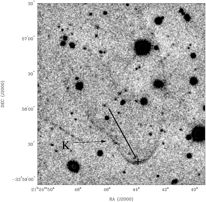
Figure 1.— NTT H$\alpha$ image of PSR J2124–3358. Counts within 40 ADU of the nebular mean have been scaled by a factor of 10 and then box-car smoothed using a $5\times 5$-pixel kernel. The cross marks the position of the pulsar at epoch MJD 52115, RA (J2000) $21^{\rm h}24^{\rm m}43\fs 8563(1)$, Dec. (J2000) $-33^{\circ}58^{\prime}44\farcs 511(3)$, while the straight line indicates the pulsar’s direction of motion in its local standard of rest. The length of the line is equal to the distance traveled by the pulsar in 1000 years. A “kink” in the bow shock is labeled with a “K”; the filament immediately to the north of the “K” is most likely not related to the pulsar.

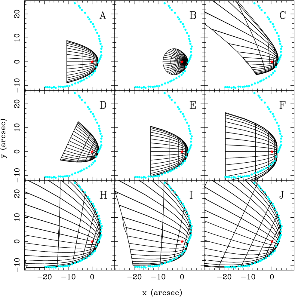
Figure 2.— Models of the bow-shock nebula powered by PSR J2124–3358. The nine panels correspond to nine of the models listed in Table 1. In each panel, the data-points (blue in the on-line version) represent the outer profile of the observed bow shock, the star (red in the on-line version) indicates the position of the pulsar, and the mesh corresponds to the surface of the model bow shock. In each case, the model bow shock solutions are plotted over the range $-140^{\circ}\leq\phi\leq 140^{\circ}$.

References

- Anantharamaiah, Radhakrishnan, & Shaver (1984) Anantharamaiah, K. R., Radhakrishnan, V., & Shaver, P. A. 1984, A&A, 138, 131.
- Bailes et al. (1997) Bailes, M. et al. 1997, ApJ, 481, 386.
- Bandiera (1993) Bandiera, R. 1993, A&A, 276, 648.
- Bell et al. (1995) Bell, J. F., Bailes, M., Manchester, R. N., Weisberg, J. M., & Lyne, A. G. 1995, ApJ, 440, L81.
- (5) Bucciantini, N. 2002a, A&A, 387, 1066.
- (6) Bucciantini, N. 2002b, A&A, 393, 629.
- Bucciantini & Bandiera (2001) Bucciantini, N. & Bandiera, R. 2001, A&A, 375, 1032.
- Chatterjee & Cordes (2002) Chatterjee, S. & Cordes, J, M. 2002, ApJ, 575, 407.
- Cordes & Lazio (2002) Cordes, J. M. & Lazio, T. J. W. 2002, preprint (astro-ph/0207156).
- Deshpande (2000) Deshpande, A. A. 2000, MNRAS, 317, 199.
- Gaensler et al. (2002) Gaensler, B. M., Arons, J., Kaspi, V. M., Pivovaroff, M. J., Kawai, N., & Tamura, K. 2002, ApJ, 569, 878.
- Hester et al. (1995) Hester, J. J. et al. 1995, ApJ, 448, 240.
- Jones, Stappers, & Gaensler (2002) Jones, D. H., Stappers, B. W., & Gaensler, B. M. 2002, A&A, 389, L1.
- Kulkarni & Fich (1985) Kulkarni, S. R. & Fich, M. 1985, ApJ, 289, 792.
- Kulkarni & Heiles (1988) Kulkarni, S. R. & Heiles, C. E. 1988, in Galactic and Extragalactic Radio Astronomy, ed. G. L. Verschuur & K. I. Kellermann, Springer–Verlag, p. 95.
- Sakurai et al. (2001) Sakurai, I., Kawai, N., Torii, K., Negoro, H., Nagase, F., Shibata, S., & Becker, W. 2001, PASJ, 53, 535.
- Toscano et al. (1999) Toscano, M., Sandhu, J. S., Bailes, M., Manchester, R. N., Britton, M. C., Kulkarni, S. R., Anderson, S. B., & Stappers, B. W. 1999, MNRAS, 307, 925.
- van der Swaluw et al. (2002) van der Swaluw, E., Achterberg, A., Gallant, Y. A., Downes, T. P., & Keppens, R. 2002, A&A, in press (astro-ph/0202232).
- Wilkin (1996) Wilkin, F. P. 1996, ApJ, 459, L31.
- Wilkin (2000) Wilkin, F. P. 2000, ApJ, 532, 400.