On the Knee in the Energy Spectrum of Cosmic Rays

Jörg R. Hörandel
University of Karlsruhe, Institut für Experimentelle Kernphysik, P.O. Box 3640, 76 021 Karlsruhe, Germany
http://www-ik.fzk.de/$\sim$joerg

Preprint arXiv:astro–ph/0210453
Submitted to Astroparticle Physics 15. April 2002; accepted 6. August 2002.

1 Introduction

After almost one century of cosmic–ray physics, a statement made by V. Hess in his Nobel Lecture in 1936 is still true: From a consideration of the immense volume of newly discovered facts in the field of physics $\ldots$ it may well appear $\ldots$ that the main problems were already solved $\ldots$. This is far from being truth, as will be shown by one of the biggest and most important newly opened fields of research, $\ldots$ that of cosmic rays [1]. Starting with very simple instruments flown in manned balloon gondolas in 1912 [2] the field developed to present–day experiments, using modern particle physics detectors at ground level, in the upper atmosphere, and in space to detect cosmic–ray particles. Many properties of cosmic rays have been clarified by these measurements, but the origin of the relativistic particles is still under discussion. Since charged particles are deflected by the irregular galactic magnetic fields, the arrival direction cannot be used to identify their sources, but measurements of their energy spectra allow to draw conclusions about their origin.

The energy spectra for individual elements are obtained directly with satellite and balloon–borne experiments at the top of the atmosphere up to several $10^{13}$ eV and for groups of elements up to $10^{15}$ eV. Due to the fast decreasing flux, measurements at higher energies require large detection areas or long exposure times, which presently can only be realized in ground–based detector systems. These experiments measure extensive air showers, generated by interactions of the high energetic cosmic rays with the nuclei in the atmosphere.

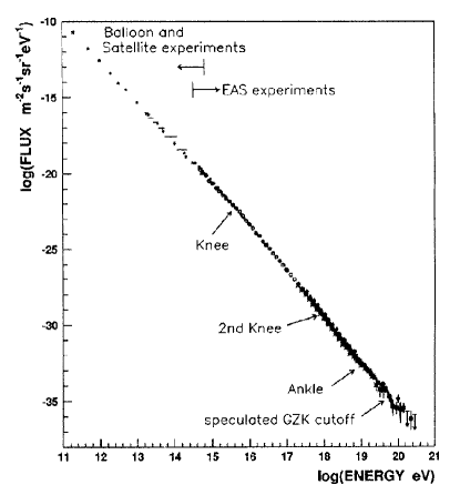
Figure 1: Cosmic–ray energy spectrum, taken from [3].

The primary energy spectrum extends over many orders of magnitude from GeV energies up to at least $10^{20}$ eV. It is a steeply falling power law spectrum with almost no structure as can be inferred from Figure 1. The only prominent features are a change in the spectral index at about 4 PeV, generally called the knee, a slight steepening around 400 PeV, designated as 2nd knee in Figure 1, and a flattening at the highest energies around 10 EeV, called the ankle. The knee was first observed by the MSU group in the electromagnetic component more than 40 years ago [4]. Since then it has been confirmed by many groups in other components of extensive air showers, viz. the electromagnetic, muonic, and hadronic component, as well as in their Čerenkov radiation. Yet its origin is still under discussion and is generally believed to be a corner stone in understanding the origin of cosmic rays.

In this article the two–knee structure is explained as a consequence of the all–particle spectrum being composed of individual spectra of elements with distinguished cut–offs. The first and prominent knee is due to the subsequent cut-offs for all elements, starting with the proton component, and the second knee marks the end of the stable elements ($Z=92$).

The idea of composing the all–particle spectrum in the knee region out of individual elemental spectra has been discussed in the literature, e.g. Webber sketches the knee in the energy spectrum as result of a rigidity dependent cut–off for individual elements [5] or Stanev et al. calculate the all-particle spectrum as sum spectrum for groups of elements from hydrogen to iron [6].

In the following the phenomenological model mentioned is described, for which the Greek notation poly gonato is chosen. In section 3 and 4 an overview is given of existing direct measurements of individual nuclei up to ultra–heavy elements which are important to explain the second knee, as well as of indirect measurements of the all–particle spectrum.

Preliminary results of this work have been presented earlier [7]. Since then, some parameters have changed due to inclusion of recent results and application of more detailed analysis procedures.

2 The Phenomenological Model

Cosmic–ray particles are most likely accelerated in strong shock fronts of supernova remnants by diffusive shock acceleration. The mechanism first introduced by Fermi [8] has been improved by many authors, see e.g. [9, 10, 11, 12, 13]. In these models particles are deflected by moving magnetized plasma clouds, the particles cross the shock front many times, and thereby gain energy up to the PeV region and achieve a nonthermal energy distribution. The Fermi acceleration at strong shocks produces a power–law spectrum close to that observed.

During the diffusive propagation of the particles through the galaxy on a random path deflected by turbulent magnetic fields, the energy spectrum of the particles is modified. The differences between source spectra and observed spectra have been explained due to nuclear spallation, leakage from the galaxy, nuclear decay, ionization losses, and, for low energies, solar modulation, see e.g. [13, 14, 15].

The poly–gonato model parametrizes the energy spectra of individual elements, based on measured data, assuming power laws and taking into account the solar modulation at low energies.

At energies in the GeV region the solar modulation of the energy spectra is described using the parametrization

$$\begin{array}[]{rl}\frac{\textstyle d\Phi_{Z}}{\textstyle dE}(E)=&N\frac{\textstyle E(E+2m_{A})}{\textstyle E+M}\cdot\\ &\frac{\textstyle\left(E+M+780\cdot e^{-2.5\cdot 10^{4}E}\right)^{\gamma_{Z}}}{\textstyle E+M+2m_{A}}\\ \end{array}$$ (1)

adopted from [23]. $N$ is a normalization constant, $\gamma_{Z}$ the spectral index of the anticipated power law at high energies (see below), $E=E_{0}/A$ the energy per nucleon, $m_{A}$ the mass of the nucleus with mass number $A$, and $M$ the solar modulation parameter. A value $M=750$ MeV is used for the parametrization.

Above about $Z\cdot 10$ GeV, the modulation due to the magnetic field of the heliosphere is negligible and the energy spectra of cosmic–ray nuclei are assumed to be described by power laws. The finite life time of supernova blast waves limits the maximum energy $E_{max}$ to be obtained during the acceleration process. The latter becomes inefficient at an energy $\hat{E}_{Z}\propto Z$, where $Z$ is the nuclear charge of the particle, and a complete cut–off is expected at the maximum energy $E_{max}$, also proportional to $Z$, see e.g. [16, 17, 18, 19]. Therefore, a cut–off or at least a change of the slope in the spectrum for the individual species at an energy $\hat{E}_{Z}\propto Z$ is expected.

In the leaky box model for cosmic–ray propagation particles are contained in a well defined volume of the galaxy, but have a small probability to escape from this volume. The gyromagnetic radius for a particle with charge $Z$, energy $E_{15}$ in PeV, and momentum $p$ in a magnetic field $B$ is given by $R=p/eZB\approx(10~{}\mbox{pc})\,E_{15}/ZB\,(\mu\mbox{G})$ [20]. In a simple picture of the propagation low $Z$ particles are more likely to escape from the galaxy as compared to particles with high $Z$ at the same energy due to their larger gyromagnetic radii.

In diffusion models, the global toroidal magnetic field in the galaxy disturbs the random walk of particles in the stochastic magnetic fields and causes a systematic drift or Hall diffusion [21]. This drift is rapidly rising with energy. It dominates at the knee the slowly increasing usual diffusion and leads to a strong leakage from the galaxy. Diffusion and drift of different nuclei at ultrarelativistic energies depend on the energy per unit charge $E_{0}/Z$, and consequently lead to a rigidity dependent cut–off for individual elements.

To summarize, both scenarios — acceleration and propagation — entail that the cut–off energy for each individual element depends on its charge $Z$. Inspired by these theories the following ansatz is adopted to describe the energy dependence of the flux for particles with charge $Z$

$$\frac{d\Phi_{Z}}{dE_{0}}(E_{0})=\Phi_{Z}^{0}E_{0}^{\gamma_{Z}}\left[1+\left(\frac{E_{0}}{\hat{E}_{Z}}\right)^{\textstyle\epsilon_{c}}\right]^{\frac{\textstyle\gamma_{c}-\gamma_{Z}}{\textstyle\epsilon_{c}}}.$$ (2)

The absolute flux $\Phi_{Z}^{0}$ and the spectral index $\gamma_{Z}$ quantify the power law. The flux above the cut–off energy is modeled by a second and steeper power law. $\gamma_{c}$ and $\epsilon_{c}$ characterize the change in the spectrum at the cut–off energy $\hat{E}_{Z}$. Both parameters are assumed to be identical for all spectra, $\gamma_{c}$ being the hypothetical slope beyond the knee and $\epsilon_{c}$ describes the smoothness of the transition from the first to the second power law. $\epsilon_{c}=1$ corresponds to a smooth change in the range of about one decade of energy, larger values describe a faster change, e.g. $\epsilon_{c}=4$ leads to a change within 1/5 of a decade.

To study systematic effects, instead of a common spectral index for all elements above the cut–off energy also a constant difference $\Delta\gamma$ between the spectral indices below and above the knee is tried and the spectrum for an element with charge $Z$ is assumed as

$$\frac{d\Phi_{Z}}{dE_{0}}(E_{0})=\Phi_{Z}^{0}E_{0}^{\gamma_{Z}}\left[1+\left(\frac{E_{0}}{\hat{E}_{Z}}\right)^{\textstyle\epsilon_{c}}\right]^{\frac{\textstyle-\Delta\gamma}{\textstyle\epsilon_{c}}}.$$ (3)

From an astrophysical point of view a rigidity dependent cut–off $\hat{E}_{Z}\propto Z$ is the most likely description, as motivated above. But, since the origin of the knee is still under discussion, also other explanations for the change of the spectral slope are possible. Some theories still favour a particle physical origin due to a change of the interactions in the atmosphere (see e.g. [22]). Such effects would probably depend on the energy per nucleon $E_{0}/A$ and lead to a nuclear mass dependent cut–off $\hat{E}_{Z}\propto A$. The last possibility considered in this article is, that the bend in the individual spectra appears at a constant energy. In the poly–gonato model all three assumptions to parametrize the cut–off energy are scrutinized.

$$\hat{E}_{Z}=\left\{\begin{array}[]{ll}\hat{E}_{p}\cdot Z&;\mbox{rigidity dependent}\\ \hat{E}_{p}\cdot A&;\mbox{mass dependent}\\ \hat{E}_{p}&;\mbox{constant}\\ \end{array}\right.$$ (4)

It will be investigated with measured data, which ansatz describes the data best. In the following, only ”poly–gonato model” refers to the rigidity dependent hypothesis.

Knowing the flux $d\Phi_{Z}/dE_{0}(E_{0})$ for the species with charge $Z$, the flux of the all–particle spectrum is obtained by summation over all cosmic–ray elements

$$\frac{d\Phi}{dE_{0}}(E_{0})=\sum_{Z=1}^{92}\frac{d\Phi_{Z}}{dE_{0}}(E_{0})\quad\mbox{.}$$ (5)

This equation contains the parameters $\Phi_{Z}^{0}$ and $\gamma_{Z}$ for each element and the common parameters, $\hat{E}_{p}$, $\epsilon_{c}$, and $\gamma_{c}$ or $\Delta\gamma$. $\Phi_{Z}^{0}$ and $\gamma_{Z}$ are obtained from direct measurements of individual nuclei. The remaining three parameters are derived from a fit to the all–particle spectrum as obtained by indirect measurements.

3 Direct Measurements

3.1 Elements with $Z\leq 28$

Many direct measurements of the energy spectra of individual cosmic–ray nuclei have been performed. Figures 2 to 4 show compilations of results for protons, helium and iron nuclei.

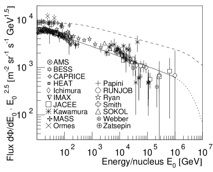
Figure 2: Differential energy spectrum for protons. The best fit to the spectrum according to a power law is represented by the solid line, the bend (dotted line) is obtained from a fit to the all–particle spectrum, see section 5. The all–particle spectrum is shown as dashed line for reference. Results are shown from AMS [24], BESS [25], CAPRICE [26], HEAT [27], Ichimura et al. [28], IMAX [29], JACEE [30], Kawamura et al. [31], MASS [32], Ormes et al. [33], Papini et al. [34], RUNJOB [35], Ryan et al. [36], Smith et al. [37], SOKOL [38], Webber et al. [39], and Zatsepin et al. [40].

The differential flux for the most abundant cosmic–ray element — hydrogen — multiplied by $E_{0}^{2.5}$ is plotted in Figure 2 versus the particle energy $E_{0}$. The data show a decreasing flux as function of energy. The straight line represents the fit according to a power law. The errors as specified by the different experiments have been taken into account. Best fit values are $\Phi_{p}^{0}=(8.73\pm 0.07)\cdot 10^{-2}~{}$ (m² s sr TeV)^-1 and $\gamma_{p}=-2.71\pm 0.02$ (solid curve) with $\chi^{2}\mbox{/d.o.f.}=3.4$. The errors specify the statistical uncertainties. The cut–off shown in the figure as dotted line will be discussed in section 5 when fitting the all–particle spectrum within the poly–gonato model. The all–particle spectrum obtained is shown for reference as well (dashed curve).

Recent measurements in the 100 GeV region, i.e. AMS, BESS, CAPRICE, and IMAX, obtain lower flux values as have been reported by earlier experiments. These values had not been available for an earlier compilation by Wiebel–Sooth et al. [16].Therefore, the flux in this reference is about 30% larger than the present result and the spectrum is slightly steeper.

When taking the experimental data in Figure 2 at face value the reader might imagine a change of slope around $10^{4}$ GeV. However, the new measurements do not confirm such former speculations. Also indirect measurements give no hint for deviations from a power law. Deriving the primary proton spectrum via the investigation of unaccompanied hadrons at mountain level, the EAS–Top experiment finds no evidence for a structure in the spectrum up to $10^{5}$ GeV [41].

Figure 3: Differential energy spectrum for helium nuclei. The best fit to the spectrum according to a power law is represented by the solid line, the bend (dotted line) is obtained from a fit to the all–particle spectrum, see section 5. The all–particle spectrum is shown as dashed line for reference. Used are values from Anand et al. [42], BESS [25], CAPRICE [26], HEAT [27], Ichimura et al. [28], IMAX [29], JACEE [30], Kawamura et al. [31], MASS [32], Ormes et al. [33], Papini et al. [34], RICH [43], RUNJOB [35], Ryan et al. [36], Smith et al. [37], SOKOL [38], and Webber et al. [39].

Figure 3 shows the differential energy spectrum for helium nuclei as a function of the total particle energy. The parameters for the spectrum, obtained by a least–square fit, are $\Phi_{He}^{0}=(5.71\pm 0.09)\cdot 10^{-2}$ (m² s sr TeV)^-1 and $\gamma_{He}=-2.64\pm 0.02$ with $\chi^{2}\mbox{/d.o.f.}=3.5$. The spectral index agrees with the value obtained by Wiebel–Sooth et al., but the absolute flux is now about 25% lower due to contributions of recent measurements, both at the low and high energy end of the spectrum.

Figure 4: Differential energy spectrum for iron nuclei. The best fit to the spectrum is represented by a solid line, the all–particle spectrum is shown as dashed line for reference. Plotted are measurements according to CRN [44], Engelmann et al. [45], Hareyama et al. [46], Ichimura et al. [28], JACEE [47], Juliusson et al. [48], Minagawa et al. [49], Orth et al. [50], RUNJOB [51], Simon et al. [52], and SOKOL [38].

As an example for heavy elements the energy spectrum for the most prominent representative — iron nuclei — is presented in Figure 4. Results from detectors which are able to resolve individual elements are given together with experiments, where the charge resolution allows only to specify the flux for the iron group, e.g. JACEE, RUNJOB, Simon et al., and SOKOL. The best fit to all measurements shown above 1 TeV yields for the power law $\Phi_{Fe}^{0}=(2.04\pm 0.26)\cdot 10^{-2}$ (m² s sr TeV)^-1 and $\gamma_{Fe}=-2.59\pm 0.06$ with $\chi^{2}\mbox{/d.o.f.}=0.9$. If the result is compared to the earlier compilation, the present absolute flux is about 15% larger, while the spectral index agrees within the specified errors with the old value. The suppression of the flux at energies below 1 TeV is due to the modulation in the heliosphere. It can be inferred from the figure, that the measurements are parametrized well using Equation (1).

Figure 5: Spectral index $\gamma_{Z}$ versus nuclear charge $Z$, see Table 7. The solid line represents a three parameter fit according to Equation (6), the dashed graph a linear fit.

Table 1: Parameters of Equation (6) for the linear and non–linear extrapolation of $\gamma_{Z}$.

	A	B	C
linear	$2.69\pm 0.12$	$(-2.07\pm 1.05)\cdot 10^{-3}$	$\equiv 1$
non–linear	$2.70\pm 0.19$	$(-8.34\pm 4.67)\cdot 10^{-4}$	$1.51\pm 0.13$

The fit parameters for protons, helium, and iron nuclei are listed together with results from Wiebel–Sooth et al. for the elements hydrogen to nickel in Table 7 in the appendix. The spectral indices for these elements are plotted in Figure 5 versus the nuclear charge. The data show a trend towards smaller values with increasing $Z$. Such a $Z$–dependence of $\gamma_{Z}$ could be explained by charge dependent effects in the acceleration or propagation process.
Theories using a nonlinear model of Fermi acceleration in supernovae remnants predict a more efficient acceleration for elements with a large mass to charge ratio as compared to elements with a smaller $A/Z$ ratio, see e.g. [53]. Consequently, it is expected that elements with higher $A/Z$ have a harder spectrum at the source.
The energy spectra observed at earth are modified during propagation of the particles through the galaxy. Some authors include reacceleration by weak interstellar shocks in the standard leaky box model, e.g. [15, 20, 54]. Like the primary acceleration also the reacceleration could be more efficient for high–$Z$–nuclei.

To estimate the fluxes of these ultra–heavy elements at high energies the parametrization

$$-\gamma_{Z}=A+B\cdot Z^{C}$$ (6)

is used to describe the $Z$ dependence of the spectral indices and to extrapolate them to higher values. To study systematic effects of the extrapolation two approaches are used, a linear function ($C\equiv 1$) and a non–linear extrapolation, using all three parameters.

The dashed line in Figure 5 represents the best fit of a linear parametrization, exhibiting a decreasing spectral index as function of the nuclear charge. The data shown in the figure exhibit some curvature which suggests to introduce the additional degree of freedom. If the parameter $C$ in Equation (6) is used as free parameter, the solid line in Figure 5 is obtained. The parameters for both trials are listed in Table 1, both fits result in about the same $\chi^{2}\mbox{/d.o.f.}\approx 2.1$. The values for the non–linear approach will be corroborated below by an independent fit to the all–particle spectrum.

3.2 Ultra–heavy elements

Figure 6: Relative abundance of cosmic–ray elements ($Z>28$) normalized to Fe$\equiv 1$ from ARIEL 6 [55], Fowler et al. [56], HEAO 3 [57], SKYLAB [58], TREK/MIR [59], Tueller et al. and Israel et al. [60], as well as UHCRE [61]. The energy is around 1 GeV/nucleon.

For ultra–heavy elements ($Z>28$) data exist only at relative low energies around a few GeV/nucleon as already mentioned. Figure 6 shows a compilation of the relative abundance from copper $(Z=29)$ up to uranium $(Z=92)$, as measured by several experiments on space crafts and balloons. The data are normalized to Fe$\equiv 1$, the threshold is about 0.5 to 1 GeV/nucleon. Some authors give only results for groups of elements, this is indicated by horizontal error bars.

The experiments ARIEL 6 [55], HEAO 3 [57], as well as Tueller et al. and Israel et al. [60] quote abundances relative to iron. Only relative abundances for elements $Z\geq 70$ are reported by Fowler et al. [56], SKYLAB [58], TREK/MIR [59], and UHCRE [61]. The results of the latter group have been normalized to ARIEL 6. This detector could resolve individual elements up to $Z=48$, and even charged nuclei above. The range $70\leq Z\leq 80$ has been used to match the abundances for Fowler et al., SKYLAB, and UHCRE. For TREK the interval $72\leq Z\leq 80$ has been utilized.

The results of all experiments show about the same structure for the relative abundances. For elements with $Z>80$ deviations are visible. Due to the very low flux only a few ($\stackrel{{\scriptstyle\textstyle<}}{{\sim}}$ 10) nuclei have been detected during a typical mission and the experiments reach their limit for statistically reliable results.

The relative abundances shown in Figure 6 are the only data available for ultra–heavy elements. No data about individual spectra are at disposal. Hence, the spectral indices for these elements have to be estimated and are obtained by extrapolating parametrization (6) to large $Z$.
The mean relative abundances for the elements are calculated from the data given in Figure 6, converted to absolute flux values and extrapolated to higher energies in the following manner. The solar modulation is taken into account using Equation (1) and the fluxes are extrapolated to 1 TeV/nucleus assuming at high energies power laws with the extrapolated spectral indices.
For $Z>48$ the detectors could only resolve even charged elements, i.e. the values shown are the sum of two elements. For the extrapolation they are split between odd and even atomic numbers using the ratio 1:5. This ratio is a typical value for the solar system composition, see Figure 7. The values thus obtained for $\Phi_{Z}^{0}$ and $\gamma_{Z}$, using the non–linear extrapolation to obtain $\gamma_{Z}$, are listed in Table 7.

3.3 Comparison with solar system composition

Figure 7: Absolute flux $\Phi_{Z}^{0}$ of cosmic–ray elements at $E_{0}=1$ TeV/nucleus versus nuclear charge according to Table 7. Two versions for the extrapolation of $\gamma_{Z}$ for ultra–heavy nuclei are indicated, see text. For comparison, solar system abundances are shown [62]. The relative values for the solar system have been normalized to the absolute flux of silicon ($Z=14$) in cosmic rays. The ordinate accounts for cosmic rays only.

The absolute flux of all cosmic–ray elements at 1 TeV/nucleus, as listed in Table 7, is plotted in Figure 7 versus the nuclear charge. For the ultra–heavy elements the linear extrapolation ($C\equiv 1$) yields slightly smaller flux values as compared to the non–linear description ($C>1$). For comparison, solar system abundances are shown as well. The relative abundances for the solar system are normalized to the absolute flux of silicon in cosmic rays. The general structure of both distributions is about the same and the differences between even and odd nuclear charge numbers are mostly visible in both compositions. However, there are differences which will be discussed next.

For cosmic rays the low abundance ”valleys” in the solar system composition around Z=4, 21, 46, and 70 are not present. This is usually believed to be the result of spallation of heavier nuclei during their propagation through the galaxy. Hydrogen, helium, and the CNO–group are suppressed in cosmic rays. This has been explained by the high first ionization potential of these atoms [63] or by the high volatility of these elements which do not condense on interstellar grains [64]. Which property is the right descriptor of cosmic–ray abundances has proved elusive, however, the volatility seems to become the more accepted solution [65].

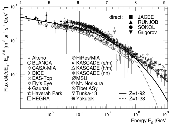
Figure 8: All–particle energy spectra obtained from direct and indirect measurements, for references see Table 2 and text. The sum spectra for individual elements according to the poly–gonato model are represented by the dotted line for $1\leq Z\leq 28$ and by the solid line for $1\leq Z\leq 92$. Above $10^{8}$ GeV the dashed line gives the normalized average spectrum.

The iron group and the ultra–heavy elements are more pronounced in cosmic rays as compared to the solar system. Especially the r–process elements beyond xenon ($Z$=54) are enhanced, partly due to spallation products of the platinum and lead nuclei ($Z$=78, 82). For the latter direct measurements at low energies around 1 GeV/n yield about a factor two more abundance as compared to the solar system and a factor of four for the actinides thorium and uranium ($Z$=90, 92) [66]. This has been attributed to the hypothesis that cosmic rays are accelerated out of supernova ejecta–enriched matter [67].

The differences for ultra–heavy elements between cosmic rays and solar system abundances seen in Figure 7 are much bigger as compared to the measurements at energies of 1 GeV/nucleon. At low energies the flux is strongly suppressed due to the solar modulation, while at 1 TeV/particle the effects of the heliospheric magnetic fields are almost negligible. Together with the enhancements discussed before, this accounts for the differences seen in Figure 7. The overall distribution from hydrogen to uranium is much flatter for cosmic rays. While the solar system abundances cover a range of 11 decades, the cosmic–ray distribution extends over 6 decades in flux only.

4 Indirect Measurements

Many groups published results on the all–particle energy spectrum from indirect measurements. Several experiments detect the main components of extensive air showers most commonly the electromagnetic component, but also muons and hadrons are investigated. The Čerenkov photons produced by relativistic shower particles and the fluorescence light of nitrogen molecules in the atmosphere induced by air showers are also utilized. The detectors are located at various atmospheric depths corresponding to altitudes from 50 m up to 4370 m a.s.l.. The experiments used in this compilation and their respective measuring techniques as well as the atmospheric overburden are listed in Table 2.

Table 2: Air shower experiments and components measured to derive the primary energy spectrum: e: electromagnetic, $\mu$: muonic, h: hadronic, Č: Čerenkov, and F: fluorescence light. The particle thresholds are given for the muonic and hadronic components. In addition, the atmospheric overburden [g/cm²] and the shift of the energy scale are listed.

Experiment	e	$\mu$	h	Č	F	g/cm2	Energy shift
AKENO (low energy) [73]	x	1 GeV				930	$-4\%$
BLANCA [74]	x			x		870	$4\%$
CASA–MIA [75]	x	800 MeV				870	$4\%$
DICE [76]	x	800 MeV		x		860	$1\%$
EAS–Top [77]	x	1 GeV				820	$-11\%$
HEGRA [78]	x			x		790	$-10\%$
KASCADE (electrons/muons) [79]	x	230 MeV				1022	$-7\%$
KASCADE (hadrons/muons) [80]		230 MeV	50 GeV			1022	$-1\%$
KASCADE (neural network) [81]	x	230 MeV				1022	$-8\%$
MSU [82]	x					1020	$-5\%$
Mt. Norikura [83]	x					735	$9\%$
Tibet [84]	x					606	$-10\%$
Tunka–13 [85]				x		680	$0\%$
Yakutsk (low energy) [86]				x		1020	$-3\%$
AKENO (high energy) [87]	x					930	$-16\%$
Fly’s Eye [88]					x	860	$-3\%$
Gauhati [89]	x					1025	$-5\%$
Haverah Park [90]	x					1018	$-10\%$
HiRes–MIA [91]		800 MeV			x	860	$-5\%$
Yakutsk (high energy) [92]	x	1 GeV		x		1020	$-20\%$

Table 3: Spectral index around 400 PeV measured by three experiments, from [88].

Experiment		energy range	spectral index		energy range	spectral index
AKENO		$10^{15.7}-10^{17.8}$ :	$3.02\pm 0.03$		$10^{17.8}-10^{18.8}$ :	$3.16\pm 0.08$
Haverah Park		$10^{17.48}-10^{17.6}$:	$3.01\pm 0.02$		$10^{17.6}-10^{18.6}$ :	$3.24\pm 0.07$
Fly’s Eye		$10^{17.3}-10^{17.6}$ :	$3.01\pm 0.06$		$10^{17.6}-10^{18.5}$ :	$3.27\pm 0.02$

Some of the experiments present different results, based on different hadronic interaction models used to interpret the data. Detailed studies of air shower properties, especially concerning the hadronic component, have been performed by the KASCADE group [69, 70]. Comparison to simulations, using the program CORSIKA [71] with several high–energy hadronic interaction models implemented revealed, that the QGSJET model presently is the best model to describe air shower data. Other groups obtained similar results, see e.g. [72, 74]. Hence, if more than one interpretation of measurements is given, the energy spectrum derived with the QGSJET model is used.

The results of the groups are presented in Figure 8. The overall agreement between the experiments is quite good, the differential fluxes multiplied by $E^{2.5}$ agree within a factor of two. All experiments exhibit a similar shape of the spectrum despite their different absolute normalization. This is remarkable since different components of air showers are investigated by various groups at different atmospheric depths, i.e. different types of particle interactions in the atmosphere are probed and the showers are sampled at different stages of their longitudinal development.

The all–particle spectrum obtained by direct measurements from JACEE [47], RUNJOB [51], SOKOL [38], and Grigorov et al. [93] agrees with the indirect measurements in the region of overlap, i.e. from below 100 TeV to 1 PeV particle energy.

Figure 9: All–particle energy spectrum at very high energies according to the Fly’s Eye experiment. The dashed line represents a fit by Bird et al. [88].

The knee at about 4 PeV is clearly recognizable in the spectrum. Assuming this bend being caused by the cut–off of the proton component, the galactic component extends in the poly–gonato model up to $Z_{U}\cdot 4$ PeV $\approx 0.4$ EeV. The energy spectrum multiplied by $E_{0}^{3}$ is shown in Figure 9 for high energies as reported by the Fly’s Eye group. Indeed, a change in the spectral slope around $4\cdot 10^{8}$ GeV is visible, the dashed line represents a fit taken from the Fly’s Eye publication [88]. A similar structure has been observed by the experiments AKENO and Haverah Park, the spectral indices obtained around 400 PeV by the three experiments are summarized in Table 3. The change coincides well with the anticipated cut–off of the heaviest nuclei of the galactic component.

5 Cosmic–ray energy spectrum

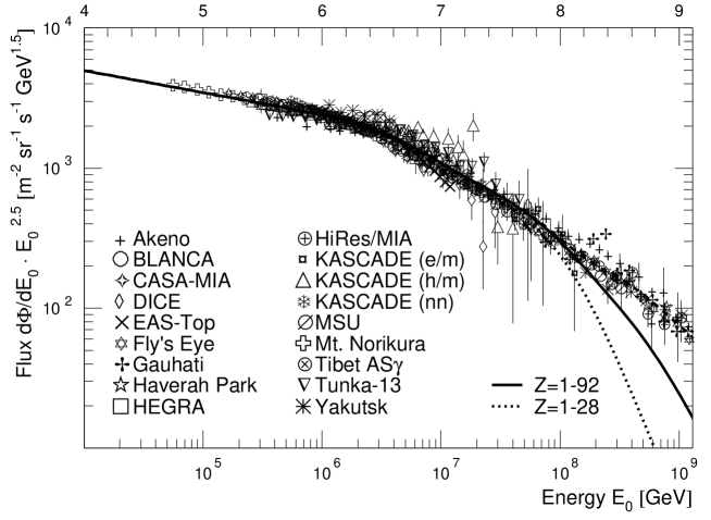
Figure 10: Normalized all–particle energy spectra for individual experiments. The renormalization values for the energy scale and references are given in Table 2. The sum spectra for individual elements according to the poly–gonato model are represented by the dotted line for $1\leq Z\leq 28$ and by the solid line for $1\leq Z\leq 92$. Above $10^{8}$ GeV the dashed line reflects the average spectrum.

The different absolute normalizations between the experiments, apparent in Figure 8, are probably caused by uncertainties in the energy calibration. The latter are quoted by the experiments to be in the order of 10% to 20%. That means the energy scales may be shifted by this amount with respect to each other. This has been done in order to elaborate a more consistent all–experiment spectrum.

5.1 Renormalization

Data from experiments which start to measure below 1 PeV have been renormalized to fit the all–particle flux at 1 PeV extrapolated from the direct measurements. The solid line in Figure 8 below 1 PeV represents the average flux of these measurements. The renormalization factors obtained are listed in Table 2 for the detector stations AKENO (low energy) to Yakutsk (low energy). Only small shifts $(\leq 11\%)$ are necessary, all within the mentioned energy uncertainties. The mean value amounts to $(-2.9\pm 1.7)\%$.

For the experiments measuring at very high energies (AKENO (high energy) to Yakutsk (high energy) in Table 2) the energy scale has been checked subsequently in the following way. The spectra have been arranged according to the lower limit of the given energy range, i.e. HiRes, AKENO, Fly’s Eye, Haverah Park, and Yakutsk, and then normalized to the average flux of all previous experiments at their lowest energies. The shape of the Gauhati energy spectrum is systematically different from all others. Therefore, it has been normalized to fit the average flux obtained by all other experiments above $10^{8}$ GeV. The energy shifts necessary are listed in Table 2, they are all negative with an average value $(-9.8\pm 2.8)\%$.

Due to differences in the shape of the spectra of individual experiments with respect to the average spectrum it is not always obvious how to normalize. This yields errors of about $\pm 2\%$ for the renormalization of the energy scales given. The average energy corrections in both groups are negative and average to $(-5.0\pm 1.6)\%$. This indicates that the experiments tend to overestimate the energy, which could be explained by a systematic effect in the hadronic interaction models applied.

The normalized spectra are shown in Figure 10. The spread between the different results has shrunk, all fluxes are contained in a narrow band. The similar shape becomes obvious in this representation, an interesting observation, since the energy scaling does not change the shape of the spectra.

The weighted average of the normalized all-particle spectra has been calculated, taking the errors of the individual measurements into account, the result is presented in Figure 11 and Table 8. The errors reflect the r.m.s. values of the data. The shape of this multi–experiment all–particle energy spectrum, already seen in Figure 10, becomes clearly apparent in this plot.

5.2 Energy dependence for the cut–off

Figure 11: Average all–particle energy spectrum. The line through the data represents a fit of the sum spectrum for elements with $1\leq Z\leq 92$ according to the poly–gonato model with rigidity dependent cut–off for a) common $\gamma_{c}$ and b) common $\Delta\gamma$. The dotted line shows the spectrum for $1\leq Z\leq 28$. In addition, energy spectra for groups of elements are shown. Above $10^{8}$ GeV the dashed line reflects the average spectrum.

Table 4: Parameters to fit the all–particle energy spectrum for the different approaches to describe the cut–off behaviour, see Equations (2) to (4), with the poly–gonato model.

$$\begin{array}[]{rcccccl}\hline\cr\mbox{cut--off:}&\mbox{rigidity}&{}{}{}\hfil&\mbox{mass}&{}{}{}\hfil&\mbox{constant}&\\ &\mbox{dependent}&&\mbox{dependent}&&&\\ \hat{E}_{Z}=&\hat{E}_{p}\cdot Z&&\hat{E}_{p}\cdot A&&\hat{E}_{p}&\\ \hline\cr\hat{E}_{p}~{}\mbox{[PeV]}=&4.51\pm 0.52&&3.66\pm 0.41&&3.50\pm 0.38&\mbox{common~{}}\gamma_{c}\\ \gamma_{c}=&-4.68\pm 0.23&&-7.82\pm 1.09&&-3.06\pm 0.02&\\ \epsilon_{c}=&1.87\pm 0.18&&2.30\pm 0.23&&1.94\pm 0.51&\\ \chi^{2}\mbox{/d.o.f}=&0.116&&0.290&&0.086&\\ \hline\cr\hat{E}_{p}~{}\mbox{[PeV]}=&4.49\pm 0.51&&3.81\pm 0.43&&3.68\pm 0.39&\mbox{common~{}}\Delta\gamma\\ \Delta\gamma=&2.10\pm 0.24&&5.70\pm 1.23&&0.44\pm 0.02&\\ \epsilon_{c}=&1.90\pm 0.19&&2.32\pm 0.22&&1.84\pm 0.45&\\ \chi^{2}\mbox{/d.o.f.}=&0.113&&0.292&&0.088&\\ \hline\cr\end{array}$$

The all–particle spectrum is used to determine the three parameters of the poly–gonato model. A least–square fit uses the values $\Phi_{Z}^{0}$ and $\gamma_{Z}$, as given in Table 7, and assumes a rigidity dependent cut–off. The two versions to model the cut–off behaviour are investigated, viz. a common spectral index $\gamma_{c}$ above the knee for all elements — Equation (2) — or a common difference in spectral slope $\Delta\gamma$ — Equation (3). The best fits obtained are shown in Figure 11 as solid lines for a common $\gamma_{c}$ (Figure 11 a) and for a common $\Delta\gamma$ (Figure 11 b). The parameters obtained are listed in the first column of Table 4.

As seen in the figure, both approaches describe the data quite well and yield low $\chi^{2}$/d.o.f. values which are given in the table. The r.m.s. values of the data have been used as errors for the fit procedure, thus the $\chi^{2}$ values obtained are $<1$. But their relative numbers are still a good quantity to characterize the different fit results. The description of the cut–off behaviour according to Equations (2) or (3) is not crucial for the results obtained. Both possibilities yield almost the same shape of the energy spectra as can be seen in Figure 11. To check systematic effects, different bin sizes for the all–particle spectrum have been tried and the upper limit of the fit range has been varied from 20 to 150 PeV. All fit results agree within the quoted errors.

To derive the energy spectra for ultra–heavy elements, the non–linear extrapolation for $\gamma_{Z}$ with $C>1$ has been used. Applying the linear extrapolation results in a sum spectrum which nearly coincides with the dotted line in Figure 11 representing the sum spectra for $1\leq Z\leq 28$. The all–particle spectrum below $10^{8}$ GeV is not effected by the choice for the extrapolation. Above this energy the contribution of the sum spectrum to the all–particle spectrum for $1\leq Z\leq 92$ is larger for the non–linear extrapolation. For example, at $5\cdot 10^{8}$ GeV the sum spectrum contributes with about 50% for the non–linear and with 12% for the linear extrapolation.

A consistency check concerning the $\gamma_{Z}$ extrapolation has been performed in the following way: The sum spectrum for $1\leq Z\leq 92$ has been fitted to the all–particle spectrum and the spectral indices for $Z>28$ have been obtained from this fit, i.e. the parameters $\hat{E}_{p}$, $\epsilon_{c}$, $\gamma_{c}$ or $\Delta\gamma$ in Equations (2) or (3) and the parameters $A$,$B$, and $C$ in Equation (6) have been determined simultaneously in a six–parameter fit. The values for both methods ($\gamma_{c}$ and $\Delta\gamma$) are consistent with the results listed in Table 4. The parameters for $\gamma_{Z}$ are almost identical to the values for the non–linear extrapolation given in Table 1. For this six–parameter fit the upper fit boundary has been varied from 30 PeV to 500 PeV. It is worth mentioning that the fit can not lower the exponents of the ultra–heavy elements even more in order to fill up the missing flux to the all–particle spectrum in the energy region above 600 PeV. The boundary of the all–particle spectrum at lower energies is the limiting factor.
That means, the values for $\gamma_{Z}$ have been derived in two independent ways, a fit of $\gamma_{Z}$ versus $Z$ in Figure 5 and in a fit of the all–particle spectrum with the poly–gonato model. Both fits yield the same results, an intriguing observation, favouring the non–linear extrapolation of $\gamma_{Z}$.

Figure 12: Average all–particle energy spectrum. The line through the data represents a fit of the sum spectrum for elements with $1\leq Z\leq 92$ according to the poly–gonato model with mass dependent cut–off for a) common $\gamma_{c}$ and b) common $\Delta\gamma$. The dotted line shows the spectrum for $1\leq Z\leq 28$. In addition, energy spectra for groups of elements are shown.

All parameters of Equation (2) and (3) being determined, the spectra of individual elements can be calculated. In order to avoid confusion not all individual spectra, but only graphs for six groups of elements are plotted in Figure 11 for demonstration. One observes that around 50 PeV about 50% of the particles should belong to the iron group and hydrogen contributes only with a few % to the all–particle flux. Indeed, the AKENO experiment [94] found when determining the mass composition from electron and muon sizes above 20 PeV that the composition becomes heavier with increasing energy. In an analysis with three mass groups (proton–helium, CNO, and iron) the amount of the light group turned out to be small, viz. in the 10% region or below around 50 PeV.

The average spectrum shows some slight structure above 4.5 PeV, i.e. it is not a pure power law. In the phenomenological approach such a shape is attributed to the sum of 92 spectra with individual cut–off energies.

Some authors, see e.g. [95], propose an additional component being necessary in addition to the known fluxes from direct observations in order to describe the all–particle energy spectrum in the knee region. It may be pointed out, that the sum spectrum of all individual elements is sufficient to compose the all–particle spectrum up to 100 PeV, as can be inferred from Figures 10 and 11. No additional cosmic–ray component is required in the knee region to explain the observed spectrum.

In order to check the two other assumptions about the cut–off behaviour of the individual element spectra — see Equation (4) — the average energy spectrum has been fitted using these two hypotheses as well.

The results for the mass dependent cut–off using Equations (2) and (3) are shown in Figure 12 and the fit values obtained are listed in the second column of Table 4. Again, the resulting spectra are essentially independent of the ansatz used to describe the spectral indices above the cut–off. The upper end of the fit range has been varied from 50 to 200 PeV, yielding consistent results.

The sum spectra obtained describe the overall shape of the spectrum less well as compared to the rigidity dependent assumption. They are below the experimental data around 3 PeV and above them around 50 PeV, this is reflected in a worse $\chi^{2}$/d.o.f. value of about a factor of 2.5 when compared to the rigidity dependent choice. Also, the steepening around the individual knees turns out to be quite different when comparing the spectra of the elemental groups in Figures 11 and 12. For the rigidity dependent cut–off the fit yields a moderate steepening, viz. a change of the slope of $\Delta\gamma=2.10$ or an index of $\gamma_{c}=-4.7$ and a smooth transition between the power laws, ranging across slightly less than one decade, with $\epsilon=1.9$.
The mass dependent ansatz results in a strong steepening of the spectra to $\gamma_{c}=-7.8$ above the knee or a change of the spectral index of $\Delta\gamma=5.7$ within a region of about half a decade ($\epsilon=2.3$). Taking the propagation of cosmic rays through the galaxy into consideration, such a sharp cut–off would be hard to explain on astrophysical grounds. Maybe a nearby cosmic–ray source, as discussed in [96], or a new type of interaction in the atmosphere could lead to such a sharp cut–off.

Figure 13: Average all–particle energy spectrum. The line through the data represents a fit of the sum spectrum for elements with $1\leq Z\leq 92$ according to the poly–gonato model with constant cut–off energy for a) common $\gamma_{c}$ and b) common $\Delta\gamma$. In addition, energy spectra for groups of elements are shown.

Using the linear extrapolation for $\gamma_{Z}$ does not improve the $\chi^{2}$–value, the spectrum around 3 PeV can not be described satisfactorily by mass–dependent cut–off energies. Nevertheless, a recent analysis, combining electromagnetic shower size spectra of several experiments favours a knee for individual elements proportional to their mass [97].

When probing the third hypothesis for the cut–off energy, the constant cut–off, the upper fit boundary has been changed from 20 to 560 PeV resulting in consistent parameters, too. The obtained spectra are plotted in Figure 13 for the two assumptions on the spectral indices above the knee and the corresponding parameters are listed in the last column of Table 4. For the common $\gamma_{c}$ the differences between the linear and the non–linear extrapolation for $\gamma_{Z}$ are negligible. For a common $\Delta\gamma$ deviations above 200 PeV are significant, as can be inferred from Figure 13 b. The non–linear extrapolation (solid line) results in larger flux values as compared to the linear extrapolation which coincides nearly with the sum spectrum for $1\leq Z\leq 28$ (dotted line).
The shape of the average energy spectrum is well described up to 200 PeV, as indicated by the low $\chi^{2}$/d.o.f. values. But the change in the spectrum at 400 PeV, seen in Figures 9 and 14, can not be described. The all–particle spectrum lies significantly above the measured values. A very smooth transition is obtained, the spectral indices change only little by $\Delta\gamma=0.4$ to a value of $\gamma_{c}=-3.1$ above the knee. The width of the transition region, described by $\epsilon=1.9$ is comparable to the one for the rigidity dependent cut–off. However, the ansatz of a constant cut–off will be disfavoured below, when discussing the resulting mean logarithmic mass.

Combining all arguments discussed, the rigidity dependent cut–off is the best choice to describe the all–particle spectrum. In the following the non–linear extrapolation for $\gamma_{Z}$ will be used together with the hypothesis of a common $\Delta\gamma$ as shown in Figure 11 b.

The resulting spectra with a rigidity dependent cut–off for protons, He, and Fe are represented in Figures 2 to 4 as solid lines with a dotted continuation in the knee region. The all–particle flux summed up from all individual elements is shown as dashed line for reference. In Figures 8 and 10 the sum spectrum of individual elements is given for $1\leq Z\leq 92$ as solid line and as dotted line for $1\leq Z\leq 28$.

Figure 14: Normalized all–particle energy spectra multiplied by $E_{0}^{3}$ for several experiments. For normalization factors and references see Table 2. The dashed line represents the average flux. The sum spectrum according to the poly–gonato model is represented by the solid line for all elements ($Z$=1–92), as well as for two elemental groups. The cut–off energy $\hat{E}_{U}=414$ PeV is marked by the pointed vertical line.

The normalized spectra for experiments investigating very high energies are shown in Figure 14 with the flux being multiplied by $E_{0}^{3}$. The slight steepening in the spectral slope around 0.4 EeV can be recognized in the results of AKENO, Fly’s Eye, Haverah Park, and HiRes/MIA. A similar steepening occurs in the Yakutsk data, but at about 4 times higher energies. Due to this unexplained systematic effect, the Yakutsk data are not taken into account when calculating the average flux. The latter is represented by a dashed line up to 3 EeV. Sum spectra for two groups of elements using a rigidity dependent cut–off with a common $\Delta\gamma$, as presented in Figure 11 b, are shown and it can be inferred, that the steepening of the spectrum coincides with the cut–off of the heaviest nuclei according to the poly–gonato model. The energy $\hat{E}_{U}=92\cdot\hat{E}_{p}=414$ PeV is marked for reference.

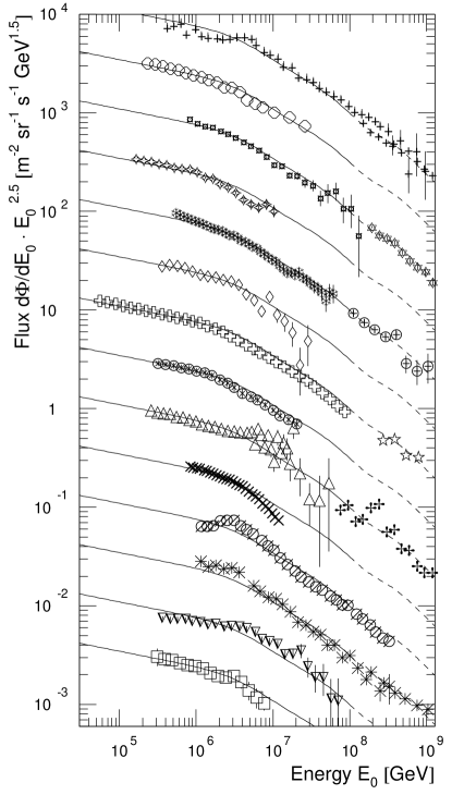
Figure 15: Normalized all–particle energy spectra for individual experiments compared to the all–particle spectrum of the poly–gonato model. The individual results are shifted in steps of half a decade in flux in order to reduce overlap.

This may lead to the conjecture, that the second knee in the all–particle spectrum is caused by the end of the galactic component of cosmic–rays, i.e. by the cut–off of the heaviest elements. At higher energies an additional component is required to account for the observed flux. For example, at 400 PeV the sum for $1\leq Z\leq 92$ accounts for about 55% of all particles. The linear extrapolation for $\gamma_{Z}$ yields a spectrum which nearly coincides with the spectrum shown for $1\leq Z\leq 28$. Figure 14 shows, that ultra–heavy elements with the non–linear dependence of $\gamma_{Z}$ on $Z$ are important to describe the measured all–particle spectrum in the region from 0.1 to 1 EeV and to explain the second knee.

In the figures presented so far it was hard to recognize the shape of the individual spectra with respect to each other. To elucidate the situation, the normalized results of the individual experiments are compared in Figure 15 to the all–particle spectrum. The solid lines represent the sum spectrum up to $10^{8}$ GeV, the dashed lines above represent the average spectrum. In order to reduce overlap between the graphs, the spectra have been shifted in flux in steps of half a decade. Different air shower components, including electrons, muons, hadrons, Čerenkov, and fluorescence photons, have been used to derive the spectra, see Table 2, and the results are compatible with the average all–particle spectrum. However, for some experiments systematic discrepancies to the all–particle spectrum can be recognized.

As the final result of the present investigations the all-particle energy spectrum derived according to the poly–gonato model with a rigidity dependent cut–off and a common $\Delta\gamma$ is given in Table 8 for reference. The differences between the calculated spectrum and the average measured flux — see Figure 11 b — are given as errors. The measurements start at 0.5 PeV in the figure, consequently, below this energy no errors are quoted. The mean relative deviation of the calculated spectrum amounts only to remarkable 3%.

6 Cosmic–ray mass composition

Figure 16: Average depth of the shower maximum $X_{max}$ versus primary energy as obtained by different experiments, for references see Table 5. Simulations taken from [112, 113] using CORSIKA/QGSJET (solid lines) and MOCCA (dashed lines) are given for primary protons and iron nuclei.

An often–used quantity to characterize the cosmic–ray mass composition above 1 PeV is the mean logarithmic mass, defined as

$$\langle\ln A\rangle=\sum_{i}r_{i}\ln A_{i}\quad,$$ (7)

$r_{i}$ being the relative fraction of nuclei of mass $A_{i}$. Some experiments derive this observable under certain assumptions from their measurements. In the superposition model of air showers, the shower development of heavy nuclei with mass $A$ and energy $E_{0}$ is described by the sum of $A$ proton showers of energy $E=E_{0}/A$. The shower maximum $t$ penetrates into the atmosphere as $t\propto\ln E$, hence, most air shower observables at ground level scale proportional to $\ln A$. Several experiments publish observables, from which the mean logarithmic mass can be derived.

Table 5: Experiments and their corresponding air shower components analyzed to derive the mean logarithmic mass: e: electromagnetic, $\mu$: muonic, h: hadronic component, Č: Čerenkov, and F: fluorescence light. The energy threshold for muons and hadrons is given. The last column lists the model used to interpret the data.

Experiment	e	$\mu~{}(E_{th})$	Č	F	model to derive $X_{max}$
BLANCA [74]	x		x		CORSIKA QGSJET
CACTI [98]	x		x		MOCCA–92
DICE [76]	x	800 MeV	x		CORSIKA VENUS
Fly’s Eye [88]				x	KNP
Haverah Park [99]	x				AIRES/SIBYLL
HEGRA (Airobic) [78]	x		x		CORSIKA QGSJET
HiRes/MIA [100]		800 MeV		x	CORSIKA QGSJET
Mt. Lian Wang [101]	x		x		MC with minijet model
SPASE/VULCAN [102]	x		x		MOCCA SIBYLL
Yakutsk [103]	x		x		QGSJET

Experiment	e	$\mu~{}(E_{th})$	h $(E_{th})$	air shower model
CASA–MIA [104]	x	800 MeV		MOCCA $\rightarrow$ QGSJET
Chacaltaya [105]	x		5 TeV	CORSIKA QGSJET
EAS–TOP/MACRO [106]	x	1.3 TeV		CORSIKA QGSJET
EAS–TOP [107]	x	1 GeV		CORSIKA QGSJET
HEGRA (CRT) [108]	x	track angle		CORSIKA VENUS
KASCADE (hadrons/muons) [109]		230 MeV	50 GeV	CORSIKA QGSJET
KASCADE (electrons/muons) [79]	x	230 MeV		CORSIKA QGSJET
KASCADE (neural network) [81]	x	230/2400 MeV	100 GeV	CORSIKA QGSJET

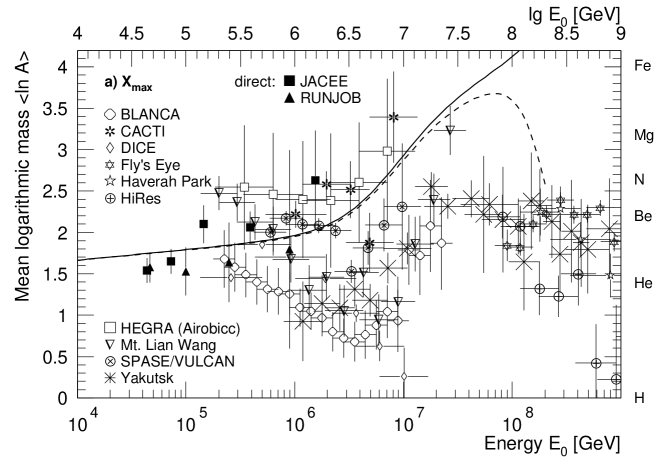
Figure 17: Mean logarithmic mass vs. primary energy. a) Results from the average depth of the shower maximum $X_{max}$ using CORSIKA/QGSJET simulations. b) Results from measurements of distributions for electrons, muons, and hadrons at ground level. For references see Table 5. Results from the balloon experiments JACEE [114] and RUNJOB [51] are given as well. Predictions according to the poly–gonato model are represented by the solid line. The dashed lines are obtained by introducing an ad–hoc component of hydrogen only, see text.

6.1 Average depth of shower maximum

A typical observable is the average depth of the shower maximum $X_{max}$ in the atmosphere. Figure 16 summarizes recent measurements using Čerenkov and fluorescence light observations. In addition, results from Haverah Park are presented. This experiment measures the electromagnetic component only, no Čerenkov or fluorescence light. $X_{max}$ is derived from the structure of the arrival time distribution and the lateral distribution of secondary particles. Characteristics of the experiments are compiled in the first part of Table 5.

The results show systematic differences of $\approx 30$ g/cm² at 1 PeV increasing to $\approx 65$ g/cm² close to 10 PeV. The strongest increase of $X_{max}$ as function of energy is reported by the DICE experiment. A recent reanalysis indicates, that part of this behaviour could be caused by systematic effects, including electronic saturation in the photomultiplier tubes, which had not been taken into account in the original analysis [110].

Only the Fly’s Eye, HiRes, and DICE experiments observe an image of the air shower and derive the average depth of the shower maximum directly. All other experiments use non–imaging techniques, i.e. the average depth of the shower maximum is derived from properties of secondary particle distributions at ground. Hence, the results obtained depend on the models used to describe the air shower development. The programs applied by different groups are listed in Table 5. Many groups use CORSIKA with the interaction models QGSJET or VENUS, but AIRES, KNP, and MOCCA are also applied. A private model including minijets is used for the Mt. Lian Wang analysis. Application of different codes can explain parts of the discrepancies in $X_{max}$. For example, Dickinson et al. found that using different interaction models in the MOCCA code, viz. the original and the SIBYLL model, the systematic error amounts to $\Delta X_{max}\approx 10$ g/cm² [102].

The measurements are compared to predictions of the shower maximum for protons and iron nuclei from simulations by Heck et al., using CORSIKA/QGSJET [112], and by Pryke, using the MOCCA code with the internal hadronic interaction model [113]. In the MOCCA model the energy is transported deeper into the atmosphere and the shower maxima are shifted by about 50 g/cm² to larger $X_{max}$ values as compared to CORSIKA/QGSJET. This results in a heavier composition. If the mean logarithmic mass is derived from $X_{max}$ according to the MOCCA simulations, the data above 10 PeV indicate a pure Fe composition. As mentioned above CORSIKA/QGSJET seems to describe the development of air showers best. Hence, in the following the QGSJET interpretation is used to derive $\langle\ln A\rangle$.

Despite of the differences mentioned, a general trend is visible in the data. All results start with an intermediate composition. However, the measured $X_{max}$ increase faster as function of energy than the model predictions, i.e. the measured values approach the proton distribution up to about 4 PeV. Above this energy, a change in the shape of the measured $X_{max}$ curves can be recognized in Figure 16 and the data start to approximate the calculations for iron nuclei with a nearest approach at about 30 PeV. Finally, at higher energies the measurements move again in direction of the proton predictions.

Knowing the average depth of the shower maximum for protons $X_{max}^{p}$ and iron nuclei $X_{max}^{Fe}$ from simulations, the mean logarithmic mass can be derived in the superposition model of air showers from the measured $X_{max}^{meas}$ using

$$\langle\ln A\rangle=\frac{X_{max}^{meas}-X_{max}^{p}}{X_{max}^{Fe}-X_{max}^{p}}\cdot\ln A_{Fe}\quad.$$ (8)

The corresponding $\langle\ln A\rangle$ values, obtained from the results shown in Figure 16, are plotted in Figure 17 a versus the primary energy. One observes a large scattering of the values. In the region 1 to 10 PeV the maximum variations amount to $\Delta\langle\ln A\rangle\approx 2$.

6.2 Particle distributions at ground level

Results on $\langle\ln A\rangle$ from experiments measuring the electromagnetic, muonic, and hadronic components at ground level are shown in Figure 17 b. The experiments and the observables used as well as the air shower model applied are listed in the second part of Table 5. The number of electrons and the number of muons are used by CASA–MIA, EAS–TOP/MACRO, and KASCADE (electrons/muons). EAS–TOP uses the number of muons at a distance of 200 m to the shower core in addition to the number of electrons. The hadronic component is analyzed by the Chacaltaya and KASCADE groups. HEGRA (CRT) measures the longitudinal shower development using the average production height of muons, i.e. the angle of incidence for individual muon tracks. Most experiments use parametric methods but also classifications on an event–by–event–basis are applied, e.g. in the KASCADE neural network analysis.

Several groups study the systematic effect caused by different interaction models. If possible, the CORSIKA QGSJET interpretation is utilized for the compilation. CASA–MIA uses MOCCA/SIBYLL simulations but in their analysis the results have been modified in order to match results from QGSJET [104].

In the KASCADE neural network analysis [81] several combinations of observables and their influence on $\langle\ln A\rangle$ have been investigated. The observables include the number of electrons, the number of muons for energy thresholds of 230 MeV and 2.4 GeV, the number of hadrons with $E_{h}>100$ GeV and their energy sum as well the spatial structure of high–energy muons. In the figure two extreme cases are shown with a difference of about 0.7 to 1.5 in $\langle\ln A\rangle$. The lower values are obtained by analyzing the number of electrons and the number of high–energy muons, while the high values result from investigations of the number of low–energy muons, the hadronic energy sum, and the spatial structure of the high–energy muons.

In another investigation of several hadronic observables by the KASCADE group the systematic differences amount to $\Delta\ln A\approx 0.4$ [109], compatible with an estimate of Swordy et al. claiming an uncertainty of $\sigma\langle\ln A\rangle\approx 0.23$ [111]. This, most likely, represents the systematic uncertainties introduced by inconsistencies in the hadronic interaction models and M.C. programs used to interpret the data.

In both graphs of Figure 17 the mean logarithmic mass calculated according to the poly–gonato model with rigidity dependent cut–off is given by the solid line. Since more and more elements reach their cut–off energy $\hat{E}_{Z}$, the mean logarithmic mass increases with rising energy and would finally reach pure uranium.

As can be seen in Figure 14 and has been discussed in section 5.2, above 100 PeV the sum spectrum for $1\leq Z\leq 92$ does not sufficiently describe the all–particle spectrum. For this reason, a new component is introduced ad hoc in order to fill the difference between the sum spectrum (solid graph) and the all–particle spectrum represented by the dashed line in Figure 14. Several theories predict an extragalactic component consisting of hydrogen and helium nuclei only, see e.g. [10]. In fact, the AKENO experiment [94] found that the mass composition becomes heavier with energy up to values of $\langle\ln A\rangle\approx 3$ at $N_{e}\approx 10^{7.5}$. For larger showers the composition gets lighter again, and in analyses with two or three mass groups the proton component recovers. The conversion of $N_{e}$ to primary energy had not been done, but cautious estimations relate $\lg N_{e}=7.5$ to about 300 PeV.

Anticipating a pure proton composition yields a lower limit for the $\langle\ln A\rangle$ values independent of any model assumptions. Hence, only protons are assumed for the ad–hoc component. The mean logarithmic mass obtained is presented in Figure 17 as dashed lines.

The results from experiments measuring electrons, muons and hadrons at ground level are in reasonable agreement with direct measurements in the region of overlap, namely below 1 PeV. Up to about 3 PeV they show a small trend of an increasing $\langle\ln A\rangle$. For higher energies the measured $\langle\ln A\rangle$ values indicate a more pronounced increase. Around 30 PeV values of $\langle\ln A\rangle\approx 3.3$, corresponding to silicon, are obtained. The prediction of the poly–gonato model yields the same shape of $\langle\ln A\rangle$ as function of energy. On the other hand, systematic differences between the results derived from the $X_{max}$ observations and the model predictions are apparent.

6.3 $X_{max}$ versus ground level observables

In order to study the difference in shape and absolute value of $\langle\ln A\rangle$ in more detail, the weighted average of $\langle\ln A\rangle$ is calculated for both, ground observables and $X_{max}$ measurements, taking into account the given errors for the individual measurements. For the calculation of $\langle\ln A\rangle$ from $X_{max}$ simulations with CORSIKA/QGSJET [112] and the MOCCA code [113] are used. Both results are shown in Figure 18 a together with the corresponding average values for ground observables in Figure 18 b. The contour lines represent the r.m.s. values of the data.

Figure 18: Average mean logarithmic mass $\langle\ln A\rangle$ vs. primary energy. Predictions of the poly–gonato model are given without and with the ad-hoc component as well as for the non–linear ($C>1$) and linear ($C\equiv 1$) extrapolation of $\gamma_{Z}$. They are compared to averaged values for experiments: a) observing $X_{max}$ using two different interaction models for the interpretation, b) measuring electrons, muons and hadrons at ground level. The contour lines represent the r.m.s. values of the data.

The parameters of the poly–gonato model have been obtained by fits to the all–particle energy spectrum. The mean logarithmic mass is an independent observable, which allows an additional check of the model. The values predicted by the model are compared to the data in Figure 18. To estimate the systematic uncertainties introduced by the extrapolation of $\gamma_{Z}$ for heavy nuclei, the mean logarithmic mass is shown for the non–linear ($C>1$) and the linear ($C\equiv 1$) extrapolation by the solid and dash dotted lines, respectively. In addition, $\langle\ln A\rangle$ values including an ad–hoc component of protons only are represented for both cases by the dashed and dotted lines, respectively. The differences between the two extrapolations for $\gamma_{Z}$ are relative small, e.g. the maximum $\langle\ln A\rangle$ values for the two cases including the ad–hoc component differ only by $\Delta\langle\ln A\rangle\approx 0.2$.

The variations of $\langle\ln A\rangle$ derived from ground observables are in the same order as the uncertainties due to the observables used. The investigations by the KASCADE group — as discussed above — suggest a systematic error of about 0.5 to 0.7 for the determination of $\langle\ln A\rangle$ compatible with the average variation of $\approx 0.5$ in Figure 18 b. The results of the poly–gonato model are in reasonable agreement with the measurements, absolute values and the shape are almost the same. Even the maximum of $\langle\ln A\rangle$ around 70 PeV is reflected by the measurements. Below 0.5 PeV only a few indirect measurements contribute, see Figure 17, and the deviations between the average data and the poly–gonato model are not to be taken seriously. Above 20 PeV the model yields a heavier composition as compared to the mean value of the measurements. It can not be excluded, that in some analysis procedures the mass values had been restricted to a range limited by the extreme values pure protons and pure iron nuclei. Therefore, the numbers at high energies could be biased towards a lighter composition.

The mean logarithmic mass derived from shower maximum observations shows for both simulation codes below the knee energy a slightly falling $\langle\ln A\rangle$. Beyond this energy $\langle\ln A\rangle$ increases, but less pronounced as compared to the ground observations. The $\langle\ln A\rangle$ values reach their maximum at about 50 PeV. This energy is in agreement with the phenomenological model, where the maximum is caused by the introduction of the ad–hoc component. As can be inferred from Figure 18 a, the results of the $X_{max}$ measurements are not compatible with the poly–gonato model. Especially below the knee they do not match the results of direct observations, nor their extrapolations to higher energies. The decreasing $\langle\ln A\rangle$ values below the knee are not seen by direct measurements. This suggests a systematic difference between ground observables and $X_{max}$ measurements which could have its origin in the air shower simulations or data analysis procedures applied. The effect is independent of the simulation program used. Both, CORSIKA and MOCCA, yield different absolute values, but the same inclined ”S” shape is obtained.

6.4 Relation for cut–off energy

Figure 19: Average mean logarithmic mass $\langle\ln A\rangle$ vs. primary energy. Predictions of the poly–gonato model with mass dependent cut–off (solid line) and with constant cut–off (dashed line) are compared to averaged experimental values. The experimental data in a) and b) are the same as in Figure 18.

The mean logarithmic mass calculated according to the poly–gonato model with mass dependent cut–off shows a similar shape but yields larger values as compared to a rigidity dependent cut-off. The results for a common $\gamma_{c}$ using the non–linear extrapolation for $\gamma_{Z}$ are plotted in Figure 19 versus the particle energy and compared to the average results of the experiments. While the $\langle\ln A\rangle$ values for the rigidity dependent cut–off are very close to the average measured results, see Figure 18 b, the values for a mass dependent cut–off above 1 PeV are about 0.3 larger than the average data. Thus, a rigidity dependent cut–off is favoured against the mass dependent approach. The hypothesis of a constant cut–off energy yields an almost constant mean logarithmic mass, as shown in Figure 19, and is not compatible with the measurements.

Combining both, the arguments discussed above in connection with the shape of the all–particle energy spectrum and the findings concerning the mean logarithmic mass, the poly–gonato model with rigidity dependent cut–off, the non–linear extrapolation of $\gamma_{Z}$, and a common $\Delta\gamma$ is the favoured solution. The $\langle\ln A\rangle$ values versus energy for this model are summarized in Table 9 for reference.

7 Compatibility with results from indirect measurements

The parameters of the poly–gonato model have been determined by extrapolating the directly measured energy spectra to high energies and a fit to the all–particle spectrum of indirect mesurements in section 5. As a first independent test, the mean logarithmic mass calculated with the poly–gonato model has been compared to experimental results in section 6. In the following, additional checks of consistency are presented. Two results from air shower measurements are compared to the predictions of the model. Namely the spectra for mass groups obtained by the KASCADE experiment [79] and $X_{max}$ distributions published by the Fly’s Eye group [115] to test the predictions in the energy regions of the knee and the cut–off for the ultra–heavy elements, respectively.

7.1 Energy spectra for groups of elements

Recently, individual spectra for groups of elements in the energy range from $10^{6}$ GeV to $10^{8}$ GeV have been reconstructed from air shower measurements by the KASCADE group [79]. Using shower size spectra for the electromagnetic and muonic component for three different zenith angle bins the primary energy spectra for elemental groups have been obtained by an unfolding procedure. Four groups, represented by hydrogen, helium, CNO, and iron have been chosen. These groups are identified with the following groups in the poly–gonato model: $Z=1$, $2\leq Z\leq 5$, $6\leq Z\leq 24$, and $25\leq Z\leq 92$. Renormalizing the KASCADE energy scale (according to Table 2 by -7%) the spectra shown in Figure 20 are obtained.

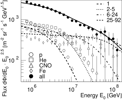
Figure 20: Energy spectra for four elemental groups and the all–particle spectrum as measured by the KASCADE experiment [79] (symbols) compared to the spectra of the poly–gonato model (lines).

The measured all–particle spectrum agrees well with the calculated flux also shown in the figure. The shapes of the experimental spectra for protons and the helium group are compatible with the spectra calculated according to the poly–gonato model. It is remarkable that the cut–off behaviour of both components agrees well with the calculated spectra, thus independently confirming the cut–off parameters obtained in section 5. The measured spectra for the CNO group and the iron group also agree with the calculations, with somewhat larger experimental error bars at high energies. In the energy region around $10^{6}$ GeV the KASCADE fluxes for protons and helium are slightly larger than in the poly–gonato model and the values for the iron group are somewhat below the calculated flux. On the whole, in an overall view the spectra of the poly–gonato model agree well with the unfolding analysis. It may be pointed out that both analyses are completely independent and they yield very similar results.

7.2 $X_{max}$–distributions

The energy region between $10^{8}$ GeV and $10^{9}$ GeV where the heaviest elements reach their cut–off energies and the ad–hoc component starts to dominate the all–particle spectrum is an interesting range for further independent tests of the predictions of the model.

Assuming protons only for the ad–hoc component, relative abundances for elemental groups are obtained as compiled in Table 6 for energies $E_{0}=3\cdot 10^{8}$ GeV, $5\cdot 10^{8}$ GeV, and $10^{9}$ GeV. In the energy range mentioned the fraction of heavy and ultra–heavy elements is expected to decrease from 62% to 35%. On the other hand the fraction of the ad–hoc component steadily increases, accounting for the rise of the light elements (protons).

Table 6: Relative abundances for groups of nuclei with charge number $Z$ for different primary energies $E_{0}$ according to the poly–gonato model. The ad–hoc component is assumed to be protons only.

		Energy $E_{0}$/GeV
	$Z$	$3\cdot 10^{8}$	$5\cdot 10^{8}$	$10^{9}$
light	1-12	38%	52%	65%
heavy	13-29	24%	12%	8%
ultra heavy	30-92	38%	36%	27%

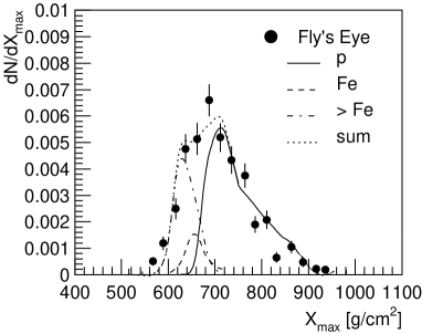
Figure 21: Distributions for the average depth of the shower maximum $X_{max}$ for different energy ranges: 3 to $5\cdot 10^{8}$ GeV (top), $5\cdot 10^{8}$ GeV to $10^{9}$ GeV (middle), and above $10^{9}$ GeV (bottom). The measured values of the Fly’s Eye experiment [115] are compared to simulated values for protons, iron and ultra–heavy nuclei, see text.

Adopting the mass composition listed in Table 6, simulations have peen performed in order to study the expected distributions of the average depth of the shower maximum $X_{max}$. The air shower simulation program CORSIKA (6.0120) with the interaction model QGSJET has been used to calculate $X_{max}$ for primary protons and iron induced showers for the energies listed in the table. For each energy and species 150 showers have been generated. The CORSIKA code allows primary nuclei with mass numbers $A\leq 56$. The $X_{max}$ distributions for ultra–heavy nuclei have been estimated using the assumption, $X_{max}\propto\ln A$, based on the simulated values for protons and iron nuclei.

In section 6.3 it has been discussed, that there are discrepancies in the mean logarithmic mass calculated from electron, muon, and hadron distributions on one hand and $X_{max}$ values on the other hand. Therefore, it can not be expected, that the CORSIKA predictions match the measured values. The distances between the lines in Figure 16 suggest, that the differences between the average $X_{max}$ values for protons and iron nuclei are almost independent from the interaction model. If a constant offset is added to the simulated values, only the absolute values of the average depths of the shower maximum are shifted but the fluctuations stay the same. Hence, to reconcile the simulations with the measured data, an offset $\Delta X_{max}=30$ g/cm² has been added to the simulated values. The resulting distributions are compared in Figure 21 to measurements of the Fly’s Eye group [115].

As can be inferred from the figure, with this offset the simulated and measured distributions are compatible with each other. For the lowest energy bin the assumption of two groups only for elements up to iron is only a crude approximation of the real mass composition and the simulation of intermediate elements like the CNO group would improve the agreement between the simulated and measured distributions. The structures on the right hand side of the proton distributions are due to fluctuations in the simulated $X_{max}$ values.

The measured showers seem to penetrate deeper into the atmosphere than predicted by the CORSIKA calculations but the width of the measured distributions, i.e. the $X_{max}$ fluctuations are well compatible with the mass composition predicted by the poly–gonato model.

8 Conclusion

An all–particle primary energy spectrum has been combined from many air shower experiments by properly adjusting the individual energy scales to meet the flux values of direct measurements. The resulting power law spectrum exhibits two changes in the spectral slope at 4.5 PeV and about 0.4 EeV.

A phenomenological model, named poly–gonato model, is adopted in which the energy spectra of individual nuclei have a power law behaviour with a cut–off at a specific energy $\hat{E}_{Z}$. The knee is explained as the subsequent cut–offs of the individual elements of the galactic component, starting with protons. The second knee seems to indicate the end of the stable elements of the galactic component.

It turns out, that the contribution of ultra–heavy elements with $Z>28$ is not negligible in the 100 PeV regime. Their flux values have been calculated, taking into consideration the modulation in the heliosphere and power law spectra, for which the spectral indices have been estimated in two independent ways.

Several assumptions about the cut–off behaviour for the individual elements have been checked against the experimental data. It turns out that the hypothesis the knee energy scales with the charge of the individual nuclei, $\hat{E}_{Z}=Z\cdot\hat{E}_{p}$, describes the data best.

Comparing several methods of extracting a mean logarithmic mass from the data indicates a systematic error of $\Delta\langle\ln A\rangle\approx 0.5$ for the determination of $\langle\ln A\rangle$. Taking this error into account, the mass composition calculated with the poly–gonato model is in agreement with results from air shower experiments measuring the electromagnetic, muonic and hadronic components at ground level. But the mass composition disagrees with results from experiments measuring the average depth of the shower maximum with Čerenkov and fluorescence detectors.

Appendix A Tables

Table 7: Absolute flux $\Phi_{Z}^{0}~{}[(\mbox{m}^{2}\mbox{~{}sr~{}s~{}TeV})^{-1}]$ at $E_{0}=1$ TeV/nucleus and spectral index $\gamma_{Z}$ of cosmic–ray elements.

$Z$		$\Phi_{Z}^{0}$	$-\gamma_{Z}$		$Z$		$\Phi_{Z}^{0}$	$-\gamma_{Z}$		$Z$		$\Phi_{Z}^{0}$	$-\gamma_{Z}$
1	H	$8.73\cdot 10^{-2}$	2.71		32	Ge	$4.02\cdot 10^{-6}$	2.54		63	Eu	$1.58\cdot 10^{-7}$	2.27
2	He	$5.71\cdot 10^{-2}$	2.64		33	As	$9.99\cdot 10^{-7}$	2.54		64	Gd	$6.99\cdot 10^{-7}$	2.25
3	Li	$2.08\cdot 10^{-3}$	2.54		34	Se	$2.11\cdot 10^{-6}$	2.53		65	Tb	$1.48\cdot 10^{-7}$	2.24
4	Be	$4.74\cdot 10^{-4}$	2.75		35	Br	$1.34\cdot 10^{-6}$	2.52		66	Dy	$6.27\cdot 10^{-7}$	2.23
5	B	$8.95\cdot 10^{-4}$	2.95		36	Kr	$1.30\cdot 10^{-6}$	2.51		67	Ho	$8.36\cdot 10^{-8}$	2.22
6	C	$1.06\cdot 10^{-2}$	2.66		37	Rb	$6.93\cdot 10^{-7}$	2.51		68	Er	$3.52\cdot 10^{-7}$	2.21
7	N	$2.35\cdot 10^{-3}$	2.72		38	Sr	$2.11\cdot 10^{-6}$	2.50		69	Tm	$1.02\cdot 10^{-7}$	2.20
8	O	$1.57\cdot 10^{-2}$	2.68		39	Y	$7.82\cdot 10^{-7}$	2.49		70	Yb	$4.15\cdot 10^{-7}$	2.19
9	F	$3.28\cdot 10^{-4}$	2.69		40	Zr	$8.42\cdot 10^{-7}$	2.48		71	Lu	$1.72\cdot 10^{-7}$	2.18
10	Ne	$4.60\cdot 10^{-3}$	2.64		41	Nb	$5.05\cdot 10^{-7}$	2.47		72	Hf	$3.57\cdot 10^{-7}$	2.17
11	Na	$7.54\cdot 10^{-4}$	2.66		42	Mo	$7.79\cdot 10^{-7}$	2.46		73	Ta	$2.16\cdot 10^{-7}$	2.16
12	Mg	$8.01\cdot 10^{-3}$	2.64		43	Tc	$6.98\cdot 10^{-8}$	2.46		74	W	$4.16\cdot 10^{-7}$	2.15
13	Al	$1.15\cdot 10^{-3}$	2.66		44	Ru	$3.01\cdot 10^{-7}$	2.45		75	Re	$3.35\cdot 10^{-7}$	2.13
14	Si	$7.96\cdot 10^{-3}$	2.75		45	Rh	$3.77\cdot 10^{-7}$	2.44		76	Os	$6.42\cdot 10^{-7}$	2.12
15	P	$2.70\cdot 10^{-4}$	2.69		46	Pd	$5.10\cdot 10^{-7}$	2.43		77	Ir	$6.63\cdot 10^{-7}$	2.11
16	S	$2.29\cdot 10^{-3}$	2.55		47	Ag	$4.54\cdot 10^{-7}$	2.42		78	Pt	$1.03\cdot 10^{-6}$	2.10
17	Cl	$2.94\cdot 10^{-4}$	2.68		48	Cd	$6.30\cdot 10^{-7}$	2.41		79	Au	$7.70\cdot 10^{-7}$	2.09
18	Ar	$8.36\cdot 10^{-4}$	2.64		49	In	$1.61\cdot 10^{-7}$	2.40		80	Hg	$7.43\cdot 10^{-7}$	2.08
19	K	$5.36\cdot 10^{-4}$	2.65		50	Sn	$7.15\cdot 10^{-7}$	2.39		81	Ti	$4.28\cdot 10^{-7}$	2.06
20	Ca	$1.47\cdot 10^{-3}$	2.70		51	Sb	$2.03\cdot 10^{-7}$	2.38		82	Pb	$8.06\cdot 10^{-7}$	2.05
21	Sc	$3.04\cdot 10^{-4}$	2.64		52	Te	$9.10\cdot 10^{-7}$	2.37		83	Bi	$3.25\cdot 10^{-7}$	2.04
22	Ti	$1.14\cdot 10^{-3}$	2.61		53	I	$1.34\cdot 10^{-7}$	2.37		84	Po	$3.99\cdot 10^{-7}$	2.03
23	V	$6.31\cdot 10^{-4}$	2.63		54	Xe	$5.74\cdot 10^{-7}$	2.36		85	At	$4.08\cdot 10^{-8}$	2.02
24	Cr	$1.36\cdot 10^{-3}$	2.67		55	Cs	$2.79\cdot 10^{-7}$	2.35		86	Rn	$1.74\cdot 10^{-7}$	2.00
25	Mn	$1.35\cdot 10^{-3}$	2.46		56	Ba	$1.23\cdot 10^{-6}$	2.34		87	Fr	$1.78\cdot 10^{-8}$	1.99
26	Fe	$2.04\cdot 10^{-2}$	2.59		57	La	$1.23\cdot 10^{-7}$	2.33		88	Ra	$7.54\cdot 10^{-8}$	1.98
27	Co	$7.51\cdot 10^{-5}$	2.72		58	Ce	$5.10\cdot 10^{-7}$	2.32		89	Ac	$1.97\cdot 10^{-8}$	1.97
28	Ni	$9.96\cdot 10^{-4}$	2.51		59	Pr	$9.52\cdot 10^{-8}$	2.31		90	Th	$8.87\cdot 10^{-8}$	1.96
29	Cu	$2.18\cdot 10^{-5}$	2.57		60	Nd	$4.05\cdot 10^{-7}$	2.30		91	Pa	$1.71\cdot 10^{-8}$	1.94
30	Zn	$1.66\cdot 10^{-5}$	2.56		61	Pm	$8.30\cdot 10^{-8}$	2.29		92	U	$3.54\cdot 10^{-7}$	1.93
31	Ga	$2.75\cdot 10^{-6}$	2.55		62	Sm	$3.68\cdot 10^{-7}$	2.28

This work, see Figures 2 to 4 and text.
From Wiebel–Sooth et al. [16].
This work, extrapolation for ultra–heavy elements, see text.

Table 8: All–particle cosmic–ray energy spectrum. Normalized average flux from air shower experiments $\Phi_{m}$ and flux $\Phi_{c}$ according to the poly–gonato model. The errors are r.m.s. values of the data for $\Phi_{m}$ and the difference between $\Phi_{m}$ and $\Phi_{c}$ for $\Phi_{c}$. ($\lg E_{0}$ [GeV] and $\Phi(E_{0})\cdot E_{0}^{2.5}~{}[\mbox{GeV}^{1.5}/\mbox{m}^{2}~{}\mbox{sr s}]$.)

$\lg E_{0}$	$\Phi_{m}(E_{0})\cdot E_{0}^{2.5}$		$\Phi_{c}(E_{0})\cdot E_{0}^{2.5}$			$\lg E_{0}$	$\Phi_{m}(E_{0})\cdot E_{0}^{2.5}$		$\Phi_{c}(E_{0})\cdot E_{0}^{2.5}$
4.0			4974			6.0	2417$\pm$	207	2395$\pm$	22
4.1			4796			6.1	2270$\pm$	212	2292$\pm$	21
4.2			4624			6.2	2164$\pm$	177	2182$\pm$	19
4.3			4459			6.3	2051$\pm$	191	2065$\pm$	15
4.4			4300			6.4	1951$\pm$	203	1939$\pm$	12
4.5			4146			6.5	1843$\pm$	230	1802$\pm$	40
4.6			3999			6.6	1680$\pm$	236	1658$\pm$	22
4.7	3911$\pm$	194	3857$\pm$	54		6.7	1519$\pm$	245	1509$\pm$	10
4.8	3841$\pm$	201	3720$\pm$	121		6.8	1368$\pm$	250	1362$\pm$	7
4.9	3711$\pm$	197	3589$\pm$	122		6.9	1229$\pm$	213	1220$\pm$	9
5.0	3579$\pm$	194	3463$\pm$	116		7.0	1076$\pm$	204	1090$\pm$	14
5.1	3427$\pm$	192	3341$\pm$	86		7.1	1011$\pm$	229	974$\pm$	38
5.2	3345$\pm$	193	3224$\pm$	121		7.2	914$\pm$	262	871$\pm$	43
5.3	3218$\pm$	191	3111$\pm$	108		7.3	815$\pm$	333	782$\pm$	33
5.4	3086$\pm$	201	3002$\pm$	85		7.4	666$\pm$	187	702$\pm$	36
5.5	2917$\pm$	251	2896$\pm$	21		7.5	586$\pm$	115	629$\pm$	43
5.6	2772$\pm$	252	2794$\pm$	22		7.6	514$\pm$	97	559$\pm$	46
5.7	2704$\pm$	237	2693$\pm$	11		7.7	461$\pm$	100	493$\pm$	33
5.8	2645$\pm$	235	2594$\pm$	50		7.8	426$\pm$	95	429$\pm$	4
5.9	2526$\pm$	217	2495$\pm$	31		7.9	353$\pm$	75	369$\pm$	16
						8.0	323$\pm$	54	314$\pm$	9

Table 9: Mean logarithmic mass according to the poly–gonato model ($\lg E_{0}$ [GeV]).

$\lg E_{0}$	$\langle\ln A\rangle$		$\lg E_{0}$	$\langle\ln A\rangle$		$\lg E_{0}$	$\langle\ln A\rangle$		$\lg E_{0}$	$\langle\ln A\rangle$
4.0	1.66		4.1	1.68		4.2	1.69		4.3	1.70
4.4	1.72		4.5	1.73		4.6	1.74		4.7	1.75
4.8	1.77		4.9	1.78		5.0	1.79		5.1	1.81
5.2	1.82		5.3	1.83		5.4	1.85		5.5	1.86
5.6	1.88		5.7	1.90		5.8	1.92		5.9	1.94
6.0	1.97		6.1	2.00		6.2	2.04		6.3	2.09
6.4	2.16		6.5	2.24		6.6	2.35		6.7	2.47
6.8	2.61		6.9	2.77		7.0	2.93		7.1	3.09
7.2	3.24		7.3	3.38		7.4	3.51		7.5	3.62
7.6	3.72-3.73		7.7	3.80-3.83		7.8	3.87-3.92		7.9	3.92-4.02
8.0	3.93-4.12		8.1	3.88-4.24		8.2	3.73-4.36		8.3	3.50-4.50

$1\leq Z\leq 92$ + ad–hoc component, protons only.
$1\leq Z\leq 92$ only.

References

- [1] V.F. Hess in Nobel Lectures in Physics 1922–1941, Elsevier (1965) 360.
- [2] V.F. Hess, Phys. Z. 13 (1912) 1084.
- [3] M. Nagano and A.A. Watson, Rev. Mod. Phys. 72 (2000) 689.
- [4] G.V. Kulikov et al., JETP 35 (1958) 635.
- [5] W.R. Webber, in Composition and Origin of Cosmic Rays, M.M. Shapiro (ed.), D. Reidel Publishing Company, Dordrecht (1983) 25.
- [6] T. Stanev et al., Astron. Astroph. 274 (1993) 902.
- [7] J.R. Hörandel, Proc. 27th Int. Cosmic Ray Conf., Hamburg 1 (2001) 71.
- [8] E. Fermi, Phys. Rev. 75 (1949) 1169.
- [9] E.G. Berezhko et al., Astrop. Phys. 7 (1997) 183.
- [10] B.L. Biermann, Astron. Astrophys. 271 (1993) 649.
- [11] L. O’C. Drury, Rep. Prog. Phys. 46 (1983) 973.
- [12] D.C. Ellison et al., Ap. J. 487 (1997) 197.
- [13] R. Blandford and D. Eichler, Physics Reports 154 (1987) 1.
- [14] C.J. Cesarsky, Ann. Rev. Astron. Astrophys. 18 (1980) 289.
- [15] J.R. Letaw et al., Ap. J. 414 (1993) 601.
- [16] B. Wiebel–Soth et al., Astron. Astroph. 330 (1998) 389.
- [17] E.G. Berezhko, Astrop. Phys. 5 (1996) 367.
- [18] P.O. Lagage et al., Astron. Astrophys. 125 (1983) 249.
- [19] H.J. Völk et al., Ap. J. 333 (1988) L65.
- [20] A. Wandel, arXiv: astro–ph/9709133.
- [21] V.S. Ptuskin et al., Astron. Astrophys. 268 (1993) 726.
- [22] S.I. Nikolsky, Nucl. Phys. B (Proc. Suppl.) 75A (1999) 217; Proc. 27th Int. Cosmic Ray Conf., Hamburg 4 (2001) 1389; S.I. Nikolsky and V.A. Romachin, Phys. Atomic Nuclei 63 (2000) 1799.
- [23] G. Bonino et al., Proc. 27th Int. Cosmic Ray Conf., Hamburg 9 (2001) 3769.
- [24] J. Alcaraz et al., Physics Lett. B 472 (2000) 215.
- [25] T. Sanuki et al., Ap. J. 545 (2000) 1135.
- [26] E. Mocchiutti et al., Proc. 27th Int. Cosmic Ray Conf., Hamburg (2001) 1634.
- [27] M.A. DuVernois et al., Proc. 27th Int. Cosmic Ray Conf., Hamburg 5 (2001) 1618.
- [28] M. Ichimura et al., Phys. Rev. D 48 (1993) 1949.
- [29] W. Menn et al., Ap. J. 533 (2000) 281.
- [30] K. Asakimori et al., Ap. J. 502 (1998) 278.
- [31] Y. Kawamura et al., Proc. 21st Int. Cosmic Ray Conf., Adelaide 3 (1990) 89.
- [32] R. Bellotti et al., Phys. Rev. D 60 (1999) 052002.
- [33] J.F. Ormes et al., Proc. 9th Int. Cosmic Ray Conf., London 1 (1965) 349.
- [34] P. Papini et al, Proc. 23rd Int. Cosmic Ray Conf., Calgary 1 (1993) 579.
- [35] A.V. Apanasenko et al., Proc. 27th Int. Cosmic Ray Conf., Hamburg 5 (2001) 1626.
- [36] M.J. Ryan et al., Phys. Rev. Lett. 28 (1972) 985.
- [37] L.H. Smith et al., Ap. J. 180 (1973) 987.
- [38] I.P. Ivanenko et al., Proc. 23rd Int. Cosmic Ray Conf., Calgary 2 (1993) 17.
- [39] W.R. Webber et al., Proc. 20th Int. Cosmic Ray Conf., Moscow 1 (1987) 325.
- [40] V.I. Zatsepin et al., Proc. 23rd Int. Cosmic Ray Conf., Calgary 2 (1993) 14.
- [41] A. Castellina et al., Proc. 27th Int. Cosmic Ray Conf., Hamburg 1 (2001) 3.
- [42] K.C. Anand et al., Proc. Ind. Acad. Sci. 67 (1968) 138.
- [43] J. Buckley et al., Ap. J. 429 (1994) 736.
- [44] D. Müller et al., Ap. J. 374 (1991) 356.
- [45] J.J. Engelmann et al., Astron. Astrophys. 148 (1985) 12.
- [46] M. Hareyama et al., 26th Int. Cosmic Ray Conf., Salt Lake City 3 (1999) 105.
- [47] K. Asakimori et al., Proc. 24th Int. Cosmic Ray Conf., Rome 2 (1995) 707 and http://marge.phys.washington.edu/ jacee/Papers/icrc95/og6.1.14.html.
- [48] E. Juliusson et al., Ap. J. 191 (1974) 331.
- [49] G. Minagawa et al., Ap. J. 248 (1981) 847.
- [50] C. Orth et al., Ap. J. 226 (1978) 1147.
- [51] A.V. Apanasenko et al., Proc. 27th Int. Cosmic Ray Conf., Hamburg 5 (2001) 1622.
- [52] M. Simon et al., Ap. J. 239 (1980) 712.
- [53] D.C. Ellison, Proc. 23rd Int. Cosmic Ray Conf., Calgary 2 (1993) 219 and D.C. Ellison et al., Ap. J. 487 (1997) 197.
- [54] A.W. Strong et al., Ap. J. 509 (1998) 212.
- [55] P.H. Fowler et al., Ap. J., 314 (1987) 739.
- [56] P.H. Fowler et al., Nucl. Instr. Meth. 147 (1977) 195.
- [57] W.R. Binns et al., Ap. J. 247 (1981) L115 and W.R. Binns et al., Ap. J. 346 (1989) 997.
- [58] E.K. Shirk et al., Ap. J. 220 (1978) 719.
- [59] B.A. Weaver et al., Proc. 27th Int. Cosmic Ray Conf., Hamburg 5 (2001) 1720.
- [60] J. Tueller et al. and M.H. Israel et al., from W.R. Binns et al., Ap. J. 247 (1981) L115.
- [61] J. Donelly et al., Proc. 26th Int. Cosmic Ray Conf., Salt Lake City 3 (1999) 109.
- [62] A.G.W. Cameron, Space Sci. Rev. 15 (1973) 121 and A.G.W. Cameron et al., Nature 243 (1973) 204 after P.K.F. Grieder, Cosmic Rays on Earth, Elsevier (2001).
- [63] R. Silberberg et al., Ap. J. 352 (1990) L49.
- [64] J.P. Meyer et al., Ap. J. 487 (1997) 182.
- [65] M.G. Baring, 26th Int. Cosmic Ray Conf., Salt Lake City, Invited, Rapporteur, and Highlight Papers, AIP Conf. Proc. 516 (2000) 153.
- [66] C.H. Tsao et al., Ap. J. 549 (2001) 320.
- [67] J.C. Higdon et al., Ap. J. 509 (1998) L33.
- [68] P.A. Mazzali et al., Astron. Astroph. 258 (1992) 399.
- [69] T. Antoni et al., J. Phys. G: Nucl. Part. Phys. 25 (1999) 2161; J.R. Hörandel et al., Proc. 26th Int. Cosmic Ray Conf., Salt Lake City 1 (1999) 131; Nucl. Phys. B (Proc. Suppl.) 75A (1999) 228.
- [70] J. Milke et al., Proc. 27th Int. Cosmic Ray Conf., Hamburg 1 (2001) 241.
- [71] D. Heck et al., Report FZKA 6019, Forschungszentrum Karlsruhe (1998); http://www-ik3.fzk.de/heck/corsika/.
- [72] A.D. Erlykin and A.W. Wolfendale, Astrop. Phys. 9 (1998) 213.
- [73] M. Nagano et al., J. Phys. G: Nucl. Part. Phys. 10 (1984) 1295.
- [74] J.W. Fowler at el., Astrop. Phys. 15 (2001) 49.
- [75] M.A.K. Glasmacher et al., Astrop. Phys. 10 (1999) 291.
- [76] S.P. Swordy and D.B. Kieda, Astrop. Phys. 13 (2000) 137.
- [77] M. Aglietta et al., Astrop. Phys. 10 (1999) 1.
- [78] F. Arqueros et al., Astron. Astrophys. 359 (2000) 682.
- [79] H. Ulrich et al., Proc. 27th Int. Cosmic Ray Conf., Hamburg 1 (2001) 97.
- [80] J.R. Hörandel et al., Proc. 26th Int. Cosmic Ray Conf., Salt Lake City 1 (1999) 337.
- [81] T. Antoni et al., Astrop. Phys. 16 (2002) 245 and M. Roth et al., Proc. 27th Int. Cosmic Ray Conf., Hamburg 1 (2001) 88.
- [82] Y.A. Fomin et al., Proc. 22nd Int. Cosmic Ray Conf., Dublin 2 (1991) 85.
- [83] N. Ito et al., Proc. 25th Int. Cosmic Ray Conf., Durban 4 (1997) 117.
- [84] M. Amenomori et al., Phys. Rev. D 62 (2000) 072007.
- [85] O.A. Gress et al., Proc. 25th Int. Cosmic Ray Conf., Durban 4 (1997) 129.
- [86] S. Knurenko et al., Proc. 27th Int. Cosmic Ray Conf., Hamburg 1 (2001) 145.
- [87] M. Nagano et al., J. Phys. G: Nucl. Part. Phys. 18 (1992) 423 and M. Teshima et al., in Astrophysical Aspects of the Most Energetic Cosmic Rays (eds. M. Nagano and F. Takahara), World Scientific (1991) 49.
- [88] D.J. Bird et al., Ap. J. 424 (1994) 491.
- [89] T. Bezboruah et al., Proc. 27th Int. Cosmic Ray Conf., Hamburg 1 (2001) 403.
- [90] M.A. Lawrence et al., J. Phys. G: Nucl. Part. Phys. 17 (1991) 733.
- [91] T. Abu-Zayyad et al., (2000) astro-ph/0010652.
- [92] N.N. Efimov et al., in Astrophysical Aspects of the Most Energetic Cosmic Rays (eds. M. Nagano and F. Takahara), World Scientific (1991) 20.
- [93] Grigorov et al., after T. Shibata, Nucl. Phys. B (Proc. Suppl.) 75A (1999) 22.
- [94] T. Hara et al., Proc. 18th Int. Cosmic Ray Conf., Bangalore 11 (1983) 285.
- [95] S.V. Ter–Antonyan et al., (2000) arXiv: hep–ex/0003006.
- [96] A.D. Erlykin and A.W. Wolfendale, Astrop. Phys. 7 (1997) 1; J. Phys G: Nucl. Part. Phys. 23 (1997) 979.
- [97] G. Schatz, Astrop. Phys. 17 (2002) 13.
- [98] S. Paling et al., Proc. 25th Int. Cosmic Ray Conf., Durban 5 (1997) 253.
- [99] A.A. Watson, Phys. Rep. 333-334 (2000) 309; J.A. Hinton et al., Proc. 26th Int. Cosmic Ray Conf., Salt Lake City 3 (1999) 288.
- [100] T. Abu–Zayyad et al., Phys. Rev. Lett. 84 (2000) 4276 and arXiv: astro–ph/9911144.
- [101] M. Cha et al., Proc. 27th Int. Cosmic Ray Conf., Hamburg 1 (2001) 132.
- [102] J.E. Dickinson et al., Proc. 26th Int. Cosmic Ray Conf., Salt Lake City 3 (1999) 136.
- [103] S. Knurenko et al., Proc. 27th Int. Cosmic Ray Conf., Hamburg 1 (2001) 177.
- [104] M.A.K. Glasmacher et al., Astrop. Phys. 12 (1999) 1.
- [105] C. Aguirre et al., Phys. Rev. D 62 (2000) 032003.
- [106] G. Navarra et al., Proc. 27th Int. Cosmic Ray Conf., Hamburg 1 (2001) 120.
- [107] B. Alessandro et al., Proc. 27th Int. Cosmic Ray Conf., Hamburg 1 (2001) 124.
- [108] K. Bernlöhr et al., Astrop. Phys. 8 (1998) 253 and K. Bernlöhr et al., Proc. 25th Int. Cosmic Ray Conf., Durban 4 (1997) 65.
- [109] J.R. Hörandel et al., Proc. 16th European Cosmic Ray Symposium, Alcala de Henares, (1998) 579; J. Engler et al., Proc. 26th Int. Cosmic Ray Conf., Salt Lake City 1 (1999) 349.
- [110] C.G. Larsen et al., Proc. 27th Int. Cosmic Ray Conf., Hamburg 1 (2001) 134.
- [111] S.P. Swordy et al., Astrop. Phys. (2002) in press.
- [112] D. Heck. et al., Proc. 27th Int. Cosmic Ray Conf., Hamburg 1 (2001) 233.
- [113] C.L. Pryke, Astrop. Phys. 14 (2001) 319.
- [114] JACEE collaboration, after T. Shibata, Nucl. Phys. B (Proc. Suppl.) 75A (1999) 22.
- [115] T.K. Gaisser et al., Phys. Rev. D 47 (1993) 1919.