Formation of large-scale semi-organized structures in turbulent convection

Abstract

A new mean-field theory of turbulent convection is developed by considering only the small-scale part of spectra as ”turbulence” and the large-scale part, as a ”mean flow”, which includes both regular and semi-organized motions. The developed theory predicts the convective wind instability in a shear-free turbulent convection. This instability causes formation of large-scale semi-organized fluid motions in the form of cells or rolls. Spatial characteristics of these motions, such as the minimum size of the growing perturbations and the size of perturbations with the maximum growth rate, are determined. This study predicts also the existence of the convective shear instability in a sheared turbulent convection. This instability causes generation of convective shear waves which have a nonzero hydrodynamic helicity. Increase of shear promotes excitation of the convective shear instability. Applications of the obtained results to the atmospheric turbulent convection and the laboratory experiments on turbulent convection are discussed. This theory can be applied also for the describing a mesogranular turbulent convection in astrophysics.

I Introduction

In the last decades it has been recognized that the very high Rayleigh number convective boundary layer (CBL) has more complex nature than might be reckoned. Besides the fully organized component naturally considered as the mean flow and the chaotic small-scale turbulent fluctuations, one more type of motion has been discovered, namely, long-lived large-scale structures, which are neither turbulent nor deterministic (see, e.g., EB93 ; AZ96 ; LS80 ; H84 ; W87 ; H88 ; SS89 ; SH89 ; M91 ; Z91 ; WH92 ; WK96 ; ZGH98 ; YKH02 ). These semi-organized structures considerably enhance the vertical transports and render them essentially non-local in nature. In the atmospheric shear-free convection, the structures represent three-dimensional Benard-type cells composed of narrow uprising plumes and wide downdraughts. They embrace the entire convective boundary layer ($\sim 2$ km in height) and include pronounced large-scale ($\sim 5$ km in diameter) convergence flow patterns close to the surface (see, e.g., EB93 ; AZ96 , and references therein). In sheared convection, the structures represent CBL-scale rolls stretched along the mean wind. Life-times of the semi-organized structures are much larger than the turbulent time scales. Thus, these structures can be treated as comparatively stable, quasi-stationary motions, playing the same role with respect to small-scale turbulence as the mean flow.

In a laboratory turbulent convection several organized features of motion, such as plumes, jets, and the large-scale circulation, are known to exist. The experimentally observed large-scale circulation in the closed box with a heated bottom wall (the Rayleigh-Benard apparatus) is often called the ”mean wind” (see, e.g., KH81 ; SWL89 ; CCL96 ; AS99 ; K01 ; NSS01 ; S94 ; BBC86 , and references therein). There are several unsolved theoretical questions concerning these flows, e.g., how do they arise, and what are their characteristics and dynamics.

In spite of a number of studies, the nature of large-scale semi-organized structures is poorly understood. The Rayleigh numbers, ${\rm Ra},$ based on the molecular transport coefficients are very large (of the order of $10^{11}-10^{13}).$ This corresponds to fully developed turbulent convection in atmospheric and laboratory flows. At the same time the effective Rayleigh numbers, ${\rm Ra}^{\rm(eff)},$ based on the turbulent transport coefficients (the turbulent viscosity and turbulent diffusivity) are not high, e.g., ${\rm Ra}^{\rm(eff)}\sim{\rm Ra}/({\rm Re}{\rm Pe}),$ where ${\rm Re}$ and ${\rm Pe}$ are the Reynolds and Peclet numbers, respectively. They are less than the critical Rayleigh numbers required for the excitation of large-scale convection. Hence the emergence of large-scale convective flows (which are observed in the atmospheric and laboratory flows) seems puzzling.

The main goal of this study is to suggest a mechanism for excitation of large-scale circulations (large-scale convection). In particular, in the present paper we develop a new mean-field theory of turbulent convection by considering only the small-scale part of spectra as ”turbulence” and the large-scale part, as a ”mean flow”, which includes both, regular and semi-organized motions. We found a convective wind instability in a shear-free turbulent convection which results in formation of large-scale semi-organized fluid motions in the form of cells or rolls (convective wind). We determined the spatial characteristics of these motions, such as the minimum size of the growing perturbations and the size of perturbations with the maximum growth rate. In addition, we studied a convective shear instability in a sheared turbulent convection which causes a generation of convective shear waves. We analyzed the relevance of the obtained results to the turbulent convection in the atmosphere and the laboratory experiments.

Traditional theoretical models of the boundary-layer turbulence, such as the Kolmogorov-type closures and similarity theories (e.g., the Monin-Obukhov surface-layer similarity theory) imply two assumptions: (i) Turbulent flows can be decomposed into two components of principally different nature: fully organized (mean-flow) and fully turbulent flows. (ii) Turbulent fluxes are uniquely determined by the local mean gradients. For example, the turbulent flux of entropy is given by

$$\langle s{\bf u}\rangle=-\kappa_{T}\mbox{\boldmath$\nabla$}\bar{S}\;$$ (1)

(see, e.g., MY75 ), where $\kappa_{T}$ is the turbulent thermal conductivity, $\bar{S}$ is the mean entropy, ${\bf u}$ and $s$ are fluctuations of the velocity and entropy.

However, the mean velocity gradients can affect the turbulent flux of entropy. The reason is that additional essentially non-isotropic velocity fluctuations can be generated by tangling of the mean-velocity gradients with the Kolmogorov-type turbulence. The source of energy of this ”tangling turbulence” is the energy of the Kolmogorov turbulence.

In the present paper we showed that the tangling turbulence can cause formation of semi-organized structures due to excitation of large-scale instability. The tangling turbulence was introduced by Wheelon W57 and Batchelor et al. BH59 for a passive scalar and by Golitsyn G60 and Moffatt M61 for a passive vector (magnetic field). Anisotropic fluctuations of a passive scalar (e.g., the number density of particles or temperature) are generated by tangling of gradients of the mean passive scalar field with random velocity field. Similarly, anisotropic magnetic fluctuations are excited by tangling of the mean magnetic field with the velocity fluctuations. The Reynolds stresses in a turbulent flow with a mean velocity shear is another example of a tangling turbulence. Indeed, they are strongly anisotropic in the presence of shear and have a steeper spectrum $(\propto k^{-7/3})$ than a Kolmogorov turbulence (see, e.g., L67 ; WC72 ; SV94 ; IY02 ). The anisotropic velocity fluctuations of tangling turbulence were studied first by Lumley L67 .

This paper is organized as follows. In Section II we described the governing equations and the method of the derivations of the turbulent flux of entropy and Reynolds stresses. In Section III using the derived mean field equations we studied the large-scale instability in a shear-free turbulent convection which causes formation of semi-organized fluid motions in the form of cells. In Section IV the instability in a sheared turbulent convection is investigated and formation of large-scale semi-organized rolls is described. Application of the obtained results for the analysis of observed semi-organized structures in the atmospheric turbulent convection is discussed in Section V.

II The governing equations and the method of the derivations

Our goal is to study the tangling turbulence, in particular, an effect of sheared large-scale motions on a developed turbulent stratified convection. To this end we consider a fully developed turbulent convection in a stratified non-rotating fluid with large Rayleigh and Reynolds numbers. The governing equations read:

$$\biggl{(}{\partial\over\partial t}+{\bf v}\cdot\mbox{\boldmath$\nabla$}\biggr{)}{\bf v} = -\mbox{\boldmath$\nabla$}\biggl{(}{P\over\rho_{0}}\biggr{)}-{\bf g}S+{\bf f}_{\nu}({\bf v})\;,$$ (2)

$$\biggl{(}{\partial\over\partial t}+{\bf v}\cdot\mbox{\boldmath$\nabla$}\biggr{)}S = -{\bf v}\cdot{\bf N}_{b}-{1\over T_{0}}\,\mbox{\boldmath$\nabla$}\cdot{\bf F}_{\kappa}(S)\;,$$ (3)

where ${\bf v}$ is the fluid velocity with $\mbox{\boldmath$\nabla$}\cdot{\bf v}={\bf\Lambda}\cdot{\bf v},$ $\,{\bf g}$ is the acceleration of gravity, $\rho_{0}{\bf f}_{\nu}({\bf v})$ is the viscous force, ${\bf F}_{\kappa}(S)$ is the heat flux that is associated with the molecular heat conductivity $\kappa,$ $\,{\bf\Lambda}=-\rho_{0}^{-1}\mbox{\boldmath$\nabla$}\rho_{0}$ is the density stratification scale, and ${\bf N}_{b}=(\gamma P_{0})^{-1}\mbox{\boldmath$\nabla$}P_{0}-\rho_{0}^{-1}\mbox{\boldmath$\nabla$}\rho_{0}.$ The variables with the subscript $"0"$ correspond to the hydrostatic equilibrium $\mbox{\boldmath$\nabla$}P_{0}=\rho_{0}{\bf g},$ and $T_{0}$ is the equilibrium fluid temperature, $S=P/\gamma P_{0}-\rho/\rho_{0}$ are the deviations of the entropy from the hydrostatic equilibrium value, $P$ and $\rho$ are the deviations of the fluid pressure and density from the hydrostatic equilibrium. Note that the variable $S=\Theta/\Theta_{0},$ where $\Theta$ is the potential temperature which is used in atmospheric physics. The Brunt-Väisälä frequency, $\Omega_{b},$ is determined by the equation $\Omega_{b}^{2}=-{\bf g}\cdot{\bf N}_{b}.$ In order to derive Eq. (2) we used an identity: $-\mbox{\boldmath$\nabla$}P+{\bf g}\rho=-\rho_{0}[\mbox{\boldmath$\nabla$}(P/\rho_{0})+{\bf g}S-P{\bf N}_{b}/\rho_{0}],$ where we assumed that $|P{\bf N}_{b}/\rho_{0}|\ll|{\bf g}S|$ and $|P{\bf N}_{b}/\rho_{0}|\ll|\mbox{\boldmath$\nabla$}(P/\rho_{0})|.$ This assumption corresponds to a nearly isentropic basic reference state when ${\bf N}_{b}$ is very small. For the derivation of this identity we also used the equation for the hydrostatic equilibrium. Equations (2) and (3) are written in the Boussinesq approximation for $\mbox{\boldmath$\nabla$}\cdot{\bf v}\not=0.$

II.1 Mean field approach

We use a mean field approach whereby the velocity, pressure and entropy are separated into the mean and fluctuating parts: ${\bf v}=\bar{\bf U}+{\bf u},$ $\,P=\bar{P}+p,$ and $S=\bar{S}+s,$ the fluctuating parts have zero mean values, $\bar{\bf U}=\langle{\bf v}\rangle,$ $\,\bar{P}=\langle P\rangle$ and $\bar{S}=\langle S\rangle.$ Averaging Eqs. (2) and (3) over an ensemble of fluctuations we obtain the mean-field equations:

$$\biggl{(}{\partial\over\partial t}+\bar{\bf U}\cdot\mbox{\boldmath$\nabla$}\biggr{)}\bar{U}_{i} = -{\nabla}_{i}\biggl{(}{\bar{P}\over\rho_{0}}\biggr{)}+(\Lambda_{j}-{\nabla}_{j})\langle u_{i}u_{j}\rangle$$ (4)

$$-{\bf g}\bar{S}+\bar{\bf f}_{\nu}(\bar{\bf U})\;,$$

$$\biggl{(}{\partial\over\partial t}+\bar{\bf U}\cdot\mbox{\boldmath$\nabla$}\biggr{)}\bar{S} = -\bar{\bf U}\cdot{\bf N}_{b}+(\Lambda_{i}-{\nabla}_{i})\langle s\,u_{i}\rangle$$ (5)

$$-{1\over T_{0}}\,\mbox{\boldmath$\nabla$}\cdot\bar{\bf F}_{\kappa}(\bar{\bf U},\bar{S})\;,$$

where $\rho_{0}\bar{\bf f}_{\nu}(\bar{\bf U})$ is the mean molecular viscous force, $\bar{\bf F}_{\kappa}(\bar{\bf U},\bar{S})$ is the mean heat flux that is associated with the molecular thermal conductivity. In order to derive a closed system of the mean-field equations we have to determine the mean-field dependencies of the Reynolds stresses $f_{ij}(\bar{\bf U},\bar{S})=\langle u_{i}(t,{\bf x})u_{j}(t,{\bf x})\rangle$ and the flux of entropy $\Phi_{i}(\bar{\bf U},\bar{S})=\langle s(t,{\bf x})u_{i}(t,{\bf x})\rangle.$ To this end we used equations for the fluctuations ${\bf u}(t,{\bf r})$ and $s(t,{\bf r})$ which are obtained by subtracting equations (4) and (5) for the mean fields from the corresponding equations (2) and (3) for the total fields:

$${\partial{\bf u}\over\partial t} = -(\bar{\bf U}\cdot\mbox{\boldmath$\nabla$}){\bf u}-({\bf u}\cdot\mbox{\boldmath$\nabla$})\bar{\bf U}-\mbox{\boldmath$\nabla$}\biggl{(}{p\over\rho_{0}}\biggr{)}$$ (6)

$$-{\bf g}\,s+{\bf U}_{N}\;,$$

$${\partial s\over\partial t} = -{\bf u}\cdot({\bf N}_{b}+\mbox{\boldmath$\nabla$}\bar{S})-(\bar{\bf U}\cdot\mbox{\boldmath$\nabla$})s+S_{N}\;,$$ (7)

where $U_{N}=\langle({\bf u}\cdot\mbox{\boldmath$\nabla$}){\bf u}\rangle-({\bf u}\cdot\mbox{\boldmath$\nabla$}){\bf u}+{\bf f}_{\nu}({\bf u})$ and $S_{N}=\langle({\bf u}\cdot\mbox{\boldmath$\nabla$})s\rangle-({\bf u}\cdot\mbox{\boldmath$\nabla$})s-(1/T_{0})\,\mbox{\boldmath$\nabla$}\cdot{\bf F}_{\kappa}({\bf u},s)$ are the nonlinear terms which include the molecular dissipative terms.

II.2 Method of derivations

By means of Eqs. (6) and (7) we determined the dependencies of the second moments $f_{ij}(\bar{\bf U},\bar{S})$ and $\Phi_{i}(\bar{\bf U},\bar{S})$ on the mean-fields $\bar{\bf U}$ and $\bar{S}.$ The procedure of the derivation is outlined in the following (for details see Appendix A).

(a). Using Eqs. (6) and (7) we derived equations for the following second moments:

$$f_{ij}({\bf k}) = \hat{L}(u_{i},u_{j})\;,\quad\Phi_{i}({\bf k})=\hat{L}(s,u_{i})\;,$$ (8)

$$F({\bf k}) = \hat{L}(s,\omega)\;,\quad G({\bf k})=\hat{L}(\omega,\omega)\;,$$ (9)

$$H({\bf k}) = \hat{L}(s,s)\;,$$ (10)

where $\hat{L}(a,b)=\langle a({\bf k})b(-{\bf k})\rangle,$ $\,\omega=(\mbox{\boldmath$\nabla$}{\bf\times}{\bf u})_{z},$ the acceleration of gravity ${\bf g}$ is directed opposite to the $z$ axis. Here we used a two-scale approach. This implies that we assumed that there exists a separation of scales, i.e., the maximum scale of turbulent motions $l_{0}$ is much smaller then the characteristic scale of inhomogeneities of the mean fields. Our final results showed that this assumption is indeed valid. The equations for the second moments (8)-(10) are given by Eqs. (53), (54) and (59)-(61) in Appendix A. In the derivation we assumed that the inverse density stratification scale $\Lambda^{2}\ll k^{2}.$

(b). The derived equations for the second moments contain the third moments, and a problem of closing the equations for the higher moments arises. Various approximate methods have been proposed for the solution of problems of this type (see, e.g., MY75 ; O70 ; Mc90 ). The simplest procedure is the $\tau$ approximation which was widely used for study of different problems of turbulent transport (see, e.g., O70 ; PFL76 ; KRR90 ; RK2000 ). One of the simplest procedures that allows us to express the third moments $f^{N}_{ij},$ ${\bf\Phi}^{N},\ldots,$ $H_{N}$ in Eqs. (53), (54) and (61) in terms of the second moments, reads

$$A_{N}({\bf k})-A_{N}^{(0)}({\bf k}) = -{A({\bf k})-A^{(0)}({\bf k})\over\tau(k)}\;,$$ (11)

where the superscript $(0)$ corresponds to the background turbulent convection (i.e., a turbulent convection with $\nabla_{i}\bar{U}_{j}=0),$ and $\tau(k)$ is the characteristic relaxation time of the statistical moments. Note that we applied the $\tau$-approximation (11) only to study the deviations from the background turbulent convection which are caused by the spatial derivatives of the mean velocity. The background turbulent convection is assumed to be known.

The $\tau$-approximation is in general similar to Eddy Damped Quasi Normal Markowian (EDQNM) approximation. However there is a principle difference between these two approaches (see O70 ; Mc90 ). The EDQNM closures do not relax to the equilibrium, and this procedure does not describe properly the motions in the equilibrium state. Within the EDQNM theory, there is no dynamically determined relaxation time, and no slightly perturbed steady state can be approached O70 . In the $\tau$-approximation, the relaxation time for small departures from equilibrium is determined by the random motions in the equilibrium state, but not by the departure from equilibrium O70 . Analysis performed in O70 showed that the $\tau$-approximation describes the relaxation to the equilibrium state (the background turbulent convection) more accurately than the EDQNM approach.

(c). We assumed that the characteristic times of variation of the second moments $f_{ij}({\bf k}),$ $\Phi_{i}({\bf k}),\ldots,$ $H({\bf k})$ are substantially larger than the correlation time $\tau(k)$ for all turbulence scales. This allowed us to determine a stationary solution for the second moments $f_{ij}({\bf k}),$ $\Phi_{i}({\bf k}),\ldots,$ $H({\bf k}).$

(d). For the integration in ${\bf k}$-space of the second moments $f_{ij}({\bf k}),$ $\Phi_{i}({\bf k}),\ldots,$ $H({\bf k})$ we have to specify a model for the background turbulent convection. Here we used the following model of the background turbulent convection which is discussed in more details in Appendix B:

$$f_{ij}^{(0)}({\bf k}) = f_{\ast}[P_{ij}({\bf k})+\varepsilon P_{ij}^{(\perp)}({\bf k}_{\perp})]\tilde{W}(k)\;,$$ (12)

$$\Phi^{(0)}_{i}({\bf k}) = k_{\perp}^{-2}[k^{2}\Phi_{z}^{(0)}({\bf k})e_{j}P_{ij}({\bf k})$$ (13)

$$+iF^{(0)}({\bf k})({\bf e}{\bf\times}{\bf k})_{i}]\;,$$

$$\Phi_{z}^{(0)}({\bf k}) = {\Phi}^{\ast}_{z}\biggl{[}2\alpha-3(\alpha-1)\biggl{(}{k_{\perp}\over k}\biggr{)}^{2}\biggr{]}\tilde{W}(k)\;,$$ (14)

$$F^{(0)}({\bf k}) = -6if^{(0)}({\bf k})({\bf\Phi}^{\ast}\cdot({\bf e}{\bf\times}{\bf k}))\;,$$ (15)

$$G^{(0)}({\bf k}) = (1+\varepsilon)f_{\ast}f^{(0)}({\bf k})k^{2}\;,$$ (16)

$$H^{(0)}({\bf k}) = 2H_{\ast}\tilde{W}(k)\;,$$ (17)

where $\tilde{W}(k)=W(k)/8\pi k^{2},$ $\,f^{(0)}({\bf k})=(k_{\perp}/k)^{2}\tilde{W}(k),$ $\,\varepsilon=(2/3)[\langle{\bf u}_{\perp}^{2}\rangle/\langle{\bf u}_{z}^{2}\rangle-2]$ is the degree of anisotropy of the turbulent velocity field ${\bf u}={\bf u}_{\perp}+u_{z}{\bf e},$ $\,\alpha$ is the degree of anisotropy of the turbulent flux of entropy (see below and Appendix B), $P_{ij}({\bf k})=\delta_{ij}-k_{ij},$ $\,k_{ij}=k_{i}k_{j}/k^{2},$ $\,{\bf k}={\bf k}_{\perp}+k_{z}{\bf e},$ $\,k_{z}={\bf k}\cdot{\bf e},$ $\,P_{ij}^{(\perp)}({\bf k}_{\perp})=\delta_{ij}-k^{\perp}_{ij}-e_{ij},$ $\,k^{\perp}_{ij}=({\bf k}_{\perp})_{i}({\bf k}_{\perp})_{j}/k_{\perp}^{2},$ $\,e_{ij}=e_{i}e_{j},\,$ ${\bf e}$ is the unit vector directed along the $z$ axis. Here $\tau(k)=2\tau_{0}\bar{\tau}(k),$ $\,W(k)=-d\bar{\tau}(k)/dk,$ $\,\bar{\tau}(k)=(k/k_{0})^{1-q},$ $\,1<q<3$ is the exponent of the kinetic energy spectrum $(q=5/3$ for Kolmogorov spectrum), $k_{0}=1/l_{0},$ and $l_{0}$ is the maximum scale of turbulent motions, $\tau_{0}=l_{0}/u_{0}$ and $u_{0}$ is the characteristic turbulent velocity in the scale $l_{0}.$ Motion in the background turbulent convection is assumed to be non-helical. In Eqs. (12) and (13) we neglected small terms $\sim O(\Lambda f_{\ast};\mbox{\boldmath$\nabla$}f_{\ast})$ and $\sim O(\Lambda\Phi^{\ast};\mbox{\boldmath$\nabla$}\Phi^{\ast}),$ respectively. Note that $f_{ij}^{(0)}({\bf k})e_{ij}=f_{\ast}f^{(0)}({\bf k}).$ Now we calculate $f_{ij}^{(0)}\equiv\int f_{ij}^{(0)}({\bf k})\,d{\bf k}$ using Eq. (12):

$$f_{ij}^{(0)}=f_{\ast}\biggl{[}{1\over 3}\delta_{ij}+{\varepsilon\over 4}(\delta_{ij}-e_{ij})\biggr{]}\;.$$ (18)

Note that ${\bf\Phi}^{(0)}\equiv\int{\bf\Phi}^{(0)}({\bf k})\,d{\bf k}={\bf\Phi}^{\ast}.$ The parameter $\alpha$ can be presented in the form

$$\alpha = {1+\xi(q+1)/(q-1)\over 1+\xi/3}\;,$$ (19)

$$\xi = (l_{\perp}/l_{z})^{q-1}-1\;,$$ (20)

where $l_{\perp}$ and $l_{z}$ are the horizontal and vertical scales in which the correlation function $\Phi_{z}^{(0)}({\bf r})=\langle s({\bf x})\,{\bf u}({\bf x}+{\bf r})\rangle$ tends to zero (see Appendix B). The parameter $\xi$ describes the degree of thermal anisotropy. In particular, when $l_{\perp}=l_{z}$ the parameter $\xi=0$ and $\alpha=1.$ For $l_{\perp}\ll l_{z}$ the parameter $\xi=-1$ and $\alpha=-3/(q-1).$ The maximum value $\xi_{\rm max}$ of the parameter $\xi$ is given by $\xi_{\rm max}=q-1$ for $\alpha=3.$ Thus, for $\alpha<1$ the thermal structures have the form of column or thermal jets $(l_{\perp}<l_{z}),$ and for $\alpha>1$ there exist the ‘’pancake” thermal structures $(l_{\perp}>l_{z})$ in the background turbulent convection. For statistically stationary small-scale turbulence the degree of anisotropy of turbulent velocity field varies in the range

$$-{\rm min}\,\biggl{\{}{4(q+3)\over 5(q+1)};\,{2(19-q)\over 25};\,{4\over 3}\biggr{\}}<\varepsilon<\infty\;.$$ (21)

The negative (positive) degree of anisotropy $\varepsilon$ of a turbulent velocity field corresponds to that the vertical size of turbulent eddies in the background turbulent convection is larger (smaller) than the horizontal size.

(e). In order to determine values $f_{\ast},$ $\,{\bf\Phi}^{\ast}$ and $\,H_{\ast}$ in the background turbulent convection we used balance equations (43)-(45) for the second moments (see Appendix A).

II.3 Turbulent flux of entropy

The procedure described in this Section allows us to determine the Reynolds stresses and turbulent flux of entropy which are given by Eqs. (71) and (72) in Appendix A, where we considered the case $\mbox{\boldmath$\nabla$}~{}\cdot~{}\bar{\bf U}=0.$ In particular, the formula for turbulent flux of entropy reads:

$${\bf\Phi}-{\bf\Phi}^{\ast} = [-5\alpha(\mbox{\boldmath$\nabla$}\cdot\bar{\bf U}_{\perp}){\bf\Phi}_{{}_{\parallel}}^{\ast}+(\alpha+3/2)(\mbox{\boldmath$\bar{\omega}$}{\bf\times}{\bf\Phi}_{{}_{\parallel}}^{\ast})$$ (22)

$$+3(\mbox{\boldmath$\bar{\omega}$}_{{}_{\parallel}}{\bf\times}{\bf\Phi}^{\ast})]{\tau_{0}(q+1)\over 15}+(\mbox{\boldmath$\nabla$}{\bf\times}{\bf T})$$

$$+({\bf E}\cdot\mbox{\boldmath$\nabla$})\bar{\bf U}\;,$$

where $\,\bar{\omega}=(\mbox{\boldmath$\nabla$}{\bf\times}\bar{\bf U})_{z},$ $\,{\bf\Phi}_{{}_{\parallel}}^{\ast}=\Phi_{z}^{\ast}{\bf e},$ $\,\mbox{\boldmath$\bar{\omega}$}_{{}_{\parallel}}=\bar{\omega}_{z}{\bf e},$ $\,{\bf T}=(2/5)\tau_{0}(q-2)({\bf\Phi}^{\ast}\cdot({\bf e}{\bf\times}\bar{\bf U}))$ and ${\bf E}=(1/5)\tau_{0}\{[2-q-2\alpha(q+1)/3]{\bf\Phi}_{{}_{\parallel}}^{\ast}-3{\bf\Phi}^{\ast}\}.$ It is shown below that the first and the second terms in Eq. (22) are responsible for the large-scale convective wind instability in a shear-free turbulent convection (see Section IV), while the third term in the turbulent flux of entropy (22) causes the convective shear instability (see Section V).

The turbulent flux of entropy can be obtained even from simple symmetry reasoning. Indeed, this flux can be presented as a sum of two terms: $\langle s{\bf u}\rangle=\Phi^{\ast}_{i}+\beta_{ijk}\nabla_{j}\bar{U}_{k},$ where ${\bf\Phi}^{\ast}$ determines the contribution of the Kolmogorov turbulence and it is independent of $\nabla_{i}\bar{U}_{j},$ whereas the second term is proportional to $\nabla_{i}\bar{U}_{j}$ and describes the contribution of the tangling turbulence. Here $\beta_{ijk}$ is an arbitrary true tensor and $\bar{\bf U}$ is the mean velocity. Using the identity $\nabla_{j}\bar{U}_{i}=(\delta\bar{\bf U})_{ij}-(1/2)\varepsilon_{ijk}\,\bar{\omega}_{k},$ the turbulent flux of entropy becomes

$$\langle su_{i}\rangle=\Phi^{\ast}_{i}+\eta_{ij}\bar{\omega}_{j}+(\mbox{\boldmath$\bar{\omega}$}{\bf\times}\mbox{\boldmath$\delta$})_{i}+\mu_{ijk}(\delta\bar{\bf U})_{jk}\;,$$ (23)

where $(\delta\bar{\bf U})_{ij}=(\nabla_{i}\bar{U}_{j}+\nabla_{j}\bar{U}_{i})/2,$ $\,\mbox{\boldmath$\bar{\omega}$}=\mbox{\boldmath$\nabla$}{\bf\times}\bar{\bf U}$ is the mean vorticity, and $\varepsilon_{ijk}$ is the fully antisymmetric Levi-Civita tensor. In Eq. (23), $\eta_{ij}$ is a symmetric pseudo-tensor, $\delta$ is a true vector, $\mu_{ijk}$ is a true tensor symmetric in the last two indexes, ${\bf\Phi}\equiv\langle s{\bf u}\rangle$ and ${\bf\Phi}^{\ast}$ are true vectors. The tensors $\eta_{ij},$ $\,\mu_{ijk}$ and the vector $\delta$ can be constructed using two vectors: ${\bf\Phi}^{\ast}$ and the vertical unit vector ${\bf e}.$ For example, $\eta_{ij}=0,$ $\mbox{\boldmath$\delta$}=A_{1}{\bf\Phi}^{\ast}+A_{2}\Phi_{z}^{\ast}{\bf e},$ and $\mu_{ijk}=A_{3}\Phi_{z}^{\ast}e_{ijk}+A_{4}\Phi_{i}^{\ast}e_{jk},$ where $A_{k}$ are the unknown coefficients and $e_{ijk}=e_{i}e_{j}e_{k}.$ This yields the following expression for the turbulent flux of entropy in a divergence-free mean velocity field:

$${\bf\Phi} = {\bf\Phi}^{\ast}-(A_{3}+A_{4})(\mbox{\boldmath$\nabla$}\cdot\bar{\bf U}_{\perp}){\bf\Phi}_{{}_{\parallel}}^{\ast}$$ (24)

$$+(A_{1}+A_{2})(\mbox{\boldmath$\bar{\omega}$}{\bf\times}{\bf\Phi}_{{}_{\parallel}}^{\ast})+A_{1}(\mbox{\boldmath$\bar{\omega}$}_{{}_{\parallel}}{\bf\times}{\bf\Phi}^{\ast})$$

$$-A_{4}(\mbox{\boldmath$\nabla$}\cdot\bar{\bf U}_{\perp}){\bf\Phi}_{\perp}^{\ast}]\;,$$

where $\bar{\bf U}=\bar{\bf U}_{\perp}+\bar{U}_{z}{\bf e},$ $\,{\bf\Phi}_{{}_{\parallel}}^{\ast}=\Phi_{z}^{\ast}{\bf e}$ and $\mbox{\boldmath$\bar{\omega}$}_{{}_{\parallel}}=\bar{\omega}_{z}{\bf e}.$ Equations  (22) and (24) coincide if one sets $A_{1}=\tau_{0}(q+1)/5,$ $\,A_{2}=\tau_{0}(q+1)(\alpha-3/2)/15,$ $\,A_{3}=\tau_{0}\alpha(q+1)/3,$ and $A_{4}=0.$ Note that $\,{\bf\Phi}^{\ast}=-\kappa_{T}\mbox{\boldmath$\nabla$}\bar{S}-\tau_{0}\Phi_{z}^{\ast}(d\bar{\bf U}^{(0)}(z)/dz),$ $\,\bar{\bf U}^{(0)}(z)$ is the imposed horizontal large-scale flow velocity (e.g., a wind velocity).

III Convective wind instability in a shear-free turbulent convection

In this section we studied the mean-field dynamics for a shear-free turbulent convection. We showed that under certain conditions a large-scale instability is excited, which causes formation of large-scale semi-organized structures in a turbulent convection.

The mean-field dynamics is determined by Eqs. (4) and (5). To study the linear stage of an instability we derived linearized equations for the small perturbations from the equilibrium, $\bar{U}_{z}^{(1)}=\bar{U}_{z}-\bar{U}_{z}^{\rm(eq)},$ $\,\bar{\omega}^{(1)}=\bar{\omega}-\bar{\omega}^{\rm(eq)}$ and $\bar{S}^{(1)}=\bar{S}-\bar{S}^{\rm(eq)}:$

$$\Delta{\partial\bar{U}_{z}^{(1)}\over\partial t} = {\partial\over\partial z}({\nabla}_{i}{\nabla}_{j}f_{ij}^{(1)})-\Delta(e_{i}{\nabla}_{j}f_{ij}^{(1)})$$ (25)

$$+g\Delta_{\perp}\bar{S}^{(1)}\;,$$

$${\partial\bar{\omega}^{(1)}\over\partial t} = -({\bf e}{\bf\times}\mbox{\boldmath$\nabla$})_{i}\left[{\nabla}_{j}f_{ij}^{(1)}+{\partial\bar{U}_{i}^{\rm(eq)}\over\partial z}\bar{U}_{z}^{(1)}\right]\;,$$ (26)

$${\partial\bar{S}^{(1)}\over\partial t} = -(\mbox{\boldmath$\nabla$}\cdot{\bf\Phi}^{(1)})-\biggl{(}N_{b}+{\partial\bar{S}^{\rm(eq)}\over\partial z}\biggr{)}\bar{U}_{z}^{(1)}\;,$$ (27)

where $\,f_{ij}^{(1)}=f_{ij}-f_{ij}^{(0)}$ and the Reynolds stresses $f_{ij}$ are given by Eqs. (71) in Appendix A, $\,\Delta_{\perp}=\Delta-\partial^{2}/\partial z^{2}$ $\,{\bf N}_{b}=N_{b}{\bf e}$ and

$$\mbox{\boldmath$\nabla$}\cdot{\bf\Phi}^{(1)} = -(\tau_{0}/30)(q+1)\{({\bf\Phi}^{\ast}\cdot{\bf e})[10\alpha\Delta_{\perp}$$ (28)

$$-(8\alpha-3)\Delta]\bar{U}_{z}^{(1)}+6(({\bf\Phi}^{\ast}{\bf\times}{\bf e})\cdot\mbox{\boldmath$\nabla$})\bar{\omega}^{(1)}\}$$

$$-\kappa_{ij}{\nabla}_{i}{\nabla}_{j}\bar{S}^{(1)}\;,$$

$$\kappa_{ij} = \tau_{0}\delta_{\ast}[f_{ij}^{(0)}+(1/2)g\tau_{0}\delta_{\ast}(4-\gamma)(e_{i}\Phi^{\ast}_{j}$$ (29)

$$+e_{j}\Phi^{\ast}_{i})]\;.$$

Equation (29) follows from Eqs. (44) and  (45).

III.1 The growth rate of convective wind instability

Let us consider a shear-free turbulent convection $(\nabla_{i}\bar{U}_{j}^{(0)}=0)$ with a given vertical flux of entropy $\Phi^{\rm(eq)}_{z}\,{\bf e}.$ We also consider an isentropic basic reference state, i.e., we neglect terms which are proportional to $(N_{b}+\partial\bar{S}^{\rm(eq)}/\partial z)\bar{U}_{z}^{(1)}$ in Eq. (27). We seek for a solution of Eqs. (25)-(27) in the form $\propto\exp(\gamma_{\rm inst}t+i{\bf K}\cdot{\bf R}),$ where ${\bf K}$ is the wave vector of small perturbations and $\gamma_{\rm inst}$ is the growth rate of the instability. Thus, the growth rate of the instability is given by

$$\gamma_{\rm inst}=\nu_{T}K^{2}A[\sqrt{1+4B/A^{2}}-1]/2\;,$$ (30)

where

$$A=B_{1}+B_{2}\;,\quad B=\beta X(c_{7}-c_{8}X)-B_{1}B_{2}\;,$$ (31)

$\,B_{1}=c_{1}+c_{6}X-c_{3}X^{2},$ $\,B_{2}=c_{4}-c_{5}X,$ $\,c_{1}=(q+3)/5,$ $\,c_{3}=\varepsilon(q+3)/4,$ $\,c_{4}=\delta_{\ast}(2+3\sigma),$ $\,c_{5}=3\delta_{\ast}(\sigma-\varepsilon/2),$ $\,c_{6}=\varepsilon(q+5)/4,$ $\,c_{7}=\mu(8\alpha-3)/10,$ $\,c_{8}=\mu\alpha,$ with $\sigma=a_{\ast}(4-\gamma)(1+\varepsilon/2),$ $\,\mu=6a_{\ast}(q+1)(1+\varepsilon/2)/\delta_{\ast},$ $\,\beta=(l_{0}K)^{-2},$ $\,X=\sin^{2}\theta,$ $\,a_{\ast}=2\delta_{\ast}\Phi^{\rm(eq)}_{z}\,g\tau_{0}/f_{\ast},$ and $\theta$ is the angle between ${\bf e}$ and the wave vector ${\bf K}$ of small perturbations. Here we used that in equilibrium $\Phi^{\rm(eq)}_{z}=\Phi^{\ast}_{z}.$ When $\beta\gg 1$ the growth rate of the instability is given by

$$\gamma_{\rm inst} \propto \nu_{T}K^{2}\,\sqrt{\mu\beta}\,|\sin\theta|\,\biggl{[}\alpha-{3\over 8}-{5\alpha\over 4}\sin^{2}\theta\biggr{]}^{1/2}$$ (32)

$$\propto Ku_{0}\;.$$

Thus for large $\beta$ the growth rate of the instability is proportional to the wave number $K$ and the instability occurs when $\alpha(5\cos^{2}\theta-1)>3/2.$ This yields two ranges for the instability:

$${3\over 2(5\cos^{2}\theta-1)}< \alpha <3\;,$$ (33)

$$-{3\over q-1}< \alpha <-{3\over 2(1-5\cos^{2}\theta)}\;,$$ (34)

where we took into account that the parameter $\alpha$ varies in the interval $-3/(q-1)<\alpha<3$ (see Appendix B). The first range for the instability in Eq. (33) is for the angles $3/10\leq\cos^{2}\theta\leq 1$ (for $q=5/3,$ the aspect ratio $0<L_{z}/L_{\perp}<1.53),$ and the second range (34) for the instability corresponds to the angles $0\leq\cos^{2}\theta<(3-q)/10$ (the aspect ratio $2.55<L_{z}/L_{\perp}<\infty),$ where $L_{z}/L_{\perp}\equiv K_{\perp}/K_{z}=\tan\theta.$ The conditions (33) and (34) correspond to $\mbox{\boldmath$\nabla$}\cdot{\bf\Phi}^{(1)}<0.$

Figure 1 demonstrates the range of parameters $L_{z}/L_{\perp}$ and $L/l_{0}$ where the instability is excited, for different values of the parameter $\alpha$ (from $-4.5$ to $3)$ and different values of the parameter $\varepsilon=-1;\,0;\,5$. Here $L\equiv 1/\sqrt{L_{z}^{-2}+L_{\perp}^{-2}}$ and we assumed that $a_{\ast}=1.$ The threshold of the instability $L_{\rm cr}$ depends on the parameter $\varepsilon.$ For example, for $\alpha=3$ the threshold of the instability $L_{\rm cr}$ varies from $3l_{0}$ to $7l_{0}$ (when $\varepsilon$ changes from $-1$ to $5).$ The negative (positive) degree of anisotropy $\varepsilon$ of turbulent velocity field corresponds to that the vertical size of turbulent eddies in the background turbulent convection is larger (smaller) than the horizontal size. The reason for the increase of the range of instability with the decrease of the degree of anisotropy $\varepsilon$ is that the rate of dissipation of the kinetic energy of the mean velocity field decreases with decrease of $\varepsilon$ and it causes decrease of the threshold of the instability. The instability does not occur when $1.53<L_{z}/L_{\perp}<2.55$ for all $\varepsilon.$

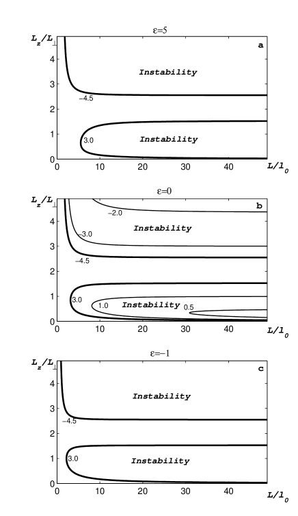
Figure 1: The range of parameters $(L_{z}/L_{\perp};L/l_{0})$ for which the convective wind instability occurs, for different values of the parameter $\alpha$: (from $-4.5$ to $3)$ and for different values of the parameter $\varepsilon$: a). $\varepsilon=5$ ; b). $\varepsilon=0$ ; c). $\varepsilon=-1.$

Figure 2 shows the growth rate of the instability as function of the parameter $L/l_{0}$ (FIG. 2a) and of the parameter $L_{z}/L_{\perp}$ (FIG. 2b) for $\varepsilon=0$ and $\alpha=2$ (the first range of the instability). This range of the instability corresponds to the ”pancake” thermal structures of the background turbulent convection $(l_{z}/l_{\perp}\approx 2/3$ for $\alpha=2).$ The maximum of the growth rate of the instability $(\gamma_{\rm max}\approx 0.045\,\tau_{0}^{-1})$ reaches at the scale of perturbations $L_{m}\approx 9.4\,l_{0}$ (for $L_{z}/L_{\perp}\approx 0.76).$ In this case the threshold of the instability $L_{\rm cr}\approx 4.2\,l_{0}.$

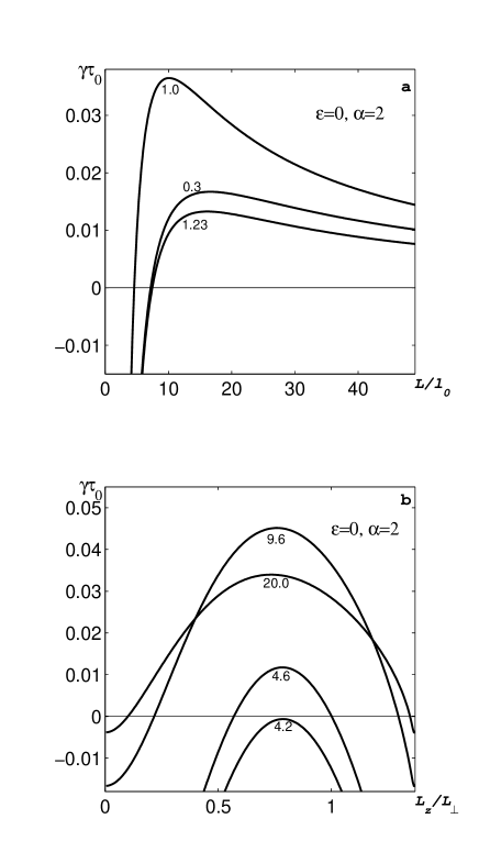
Figure 2: The growth rate of the convective wind instability as functions of: a). $L/l_{0}$ (for different values of parameter $L_{z}/L_{\perp}=0.3;\,1;\,1.23);$ and b). $L_{z}/L_{\perp}$ (for different values of parameter $L/l_{0}=4.2;\,4.6;\,9.6;\,20)$ for $\varepsilon=0$ and $\alpha=2$.

Figure 3 demonstrates the growth rate for the second range of the instability $(\alpha=-3).$ Note that this range of the instability corresponds to the thermal structures of the background turbulent convection in the form of columns $(l_{z}/l_{\perp}\approx 2$ for $\alpha=-3).$ In contrast to the first range of the instability, the growth rate increases with $L_{z}/L_{\perp}$ in the whole second range of the instability (see FIG. 3b).

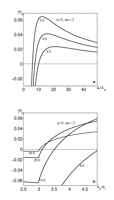
Figure 3: The growth rate of the convective wind instability as functions of: a). $L/l_{0}$ (for different values of parameter $L_{z}/L_{\perp}=3.5;\,4;\,5);$ and b). $L_{z}/L_{\perp}$ (for different values of parameter $L/l_{0}=6;\,10;\,20;\,40);$ for $\varepsilon=5$ and $\alpha=-3.$

III.2 Mechanism of the convective wind instability

The convective wind instability results in formation of large-scale semi-organized structures in the form of cells (convective wind) in turbulent convection. The mechanism of the convective wind instability, associated with the first term ${\bf\Phi}\propto-\tau_{0}\alpha(\mbox{\boldmath$\nabla$}\cdot\bar{\bf U}_{\perp}){\bf\Phi}_{{}_{\parallel}}^{\ast}$ in the expression for the turbulent flux of entropy [see Eq. (22)], in the shear-free turbulent convection at $\alpha>0$ is as follows. Perturbations of the vertical velocity $\bar{U}_{z}$ with $\partial\bar{U}_{z}/\partial z>0$ have negative divergence of the horizontal velocity , i.e., ${\rm div}\,\bar{\bf U}_{\perp}<0$ (provided that ${\rm div}\,\bar{\bf U}\approx 0).$ This results in the vertical turbulent flux of entropy $\tilde{\Phi}_{z}\propto-{\rm div}\,\bar{\bf U}_{\perp}$, and it causes an increase of the mean entropy $(\bar{S}\propto\beta^{-1/2}\,\bar{U}_{z}\Phi^{\ast}/u_{0}^{2})$ [see Eqs. (27)-(28) and (32)].

On the other hand, the increase of the the mean entropy increases the buoyancy force $\propto g\bar{S}$ and results in the increase of the vertical velocity $\bar{U}_{z}\propto\tau_{0}\beta^{1/2}\,g\bar{S}$ and excitation of the large-scale instability [see Eqs. (25) and (32)]. Similar phenomenon occurs in the regions with $\partial\bar{U}_{z}/\partial z<0$ whereby ${\rm div}\,\bar{\bf U}_{\perp}>0.$ This causes a downward flux of the entropy and the decrease of the mean entropy. The latter enhances the downward flow and results in the instability which causes formation of a large-scale semi-organized convective wind structure. Thus, nonzero ${\rm div}\,\bar{\bf U}_{\perp}$ causes redistribution of the vertical turbulent flux of entropy and formation of regions with large vertical fluxes of entropy (see FIG. 4). This results in a formation of a large-scale circulation of the velocity field. This mechanism determines the first range for the instability.

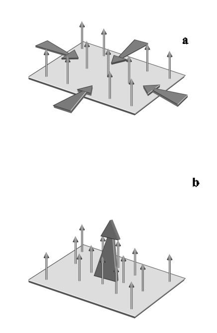
Figure 4: The effect of a nonzero ${\rm div}\,\bar{\bf U}_{\perp}$ which causes a redistribution of the vertical turbulent flux of the entropy and results in a formation of a large-scale circulation of the velocity field. Fluid flow with ${\rm div}\,\bar{\bf U}_{\perp}<0$ (a) produces regions with vertical fluxes of entropy and vertical fluid flow (b) in these regions.

The large-scale circulation of the velocity field causes a nonzero mean vorticity $\bar{\omega},$ and the second term [proportional to $(\alpha+3/2)(\mbox{\boldmath$\bar{\omega}$}{\bf\times}{\bf\Phi}_{{}_{\parallel}}^{\ast})]$ in the turbulent flux of the entropy (22) is responsible for a formation of a horizontal turbulent flux of the entropy. This causes a decrease of the growth rate of the convective wind instability (for $\alpha>0),$ because it decreases the mean entropy $\bar{S}$ in the regions with $\partial\bar{U}_{z}/\partial z>0.$ The net effect is determined by a competition between these effects which are described by the first and the second terms in the turbulent flux of the entropy (22). The latter determines a lower positive limit $\alpha_{\rm min}=3/8$ of the parameter $\alpha.$

When $\alpha<-3/2$ the signs of the first and second terms in the expression (22) for the turbulent flux of entropy change. Thus, another mechanism of the convective wind instability is associated with the second term in the expression (22) for the turbulent flux of entropy when $\alpha<-3/2.$ This term describes the horizontal flux of the mean entropy ${\bf\Phi}_{y}\propto\tau_{0}(\alpha+3/2)(\mbox{\boldmath$\bar{\omega}$}{\bf\times}{\bf\Phi}_{{}_{\parallel}}^{\ast}).$ The latter results in the increase (decrease) of the mean entropy in the regions with upward (downward) fluid flows (see FIG. 5). On the other hand, the increase of the mean entropy results in the increase of the buoyancy force, the mean vertical velocity $\bar{U}_{z}$ and the mean vorticity $\mbox{\boldmath$\bar{\omega}$}.$ The latter amplifies the horizontal turbulent flux of entropy ${\bf\Phi}_{y}$ and causes the large-scale convective wind instability. This mechanism determines the second range for the convective wind instability. The first term in the turbulent flux of entropy at $\alpha<0$ causes a decrease of the growth rate of the instability because, when $\alpha<0,$ it implies a downward turbulent flux of entropy in the upward flow. This decreases both, the mean entropy and the buoyancy force. Note that, when $\alpha<-3/2,$ the thermal structure of the background turbulence has the form of a thermal column or jets: $l_{z}/l_{\perp}>3.34.$ Even for $\alpha<0,$ the ratio $l_{z}/l_{\perp}>1.54.$

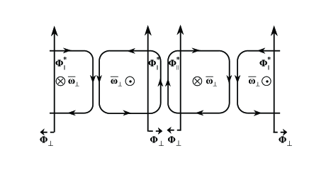
Figure 5: The effect of a nonzero $\mbox{\boldmath$\bar{\omega}$}{\bf\times}{\bf\Phi}_{{}_{\parallel}}^{\ast}$ which induces the horizontal flux of the mean entropy ${\bf\Phi}_{y}$ and causes increase (decrease) the mean entropy in the regions with upward (downward) fluid flow when $\alpha<-3/2.$

IV Convective shear instability

Let us consider turbulent convection with a linear shear $\bar{\bf U}^{(0)}=(\lambda/\tau_{0})\,z\,{\bf e}_{y}$ and a nonzero vertical flux of entropy ${\bf\Phi}=\Phi^{\rm(eq)}_{z}\,{\bf e},$ where $\lambda$ is dimensionless parameter which characterizes the shear. We also consider an isentropic basic reference state, i.e., we neglected a term which is proportional to $(N_{b}+\partial\bar{S}^{\rm(eq)}/\partial z)\bar{U}_{z}^{(1)}$ in Eq. (27). We seek for a solution of Eqs. (25)-(27) in the form $\bar{\bf U}^{(1)}=\bar{\bf V}\exp(\gamma_{\rm inst}t)\cos(\Omega t+{\bf K}\cdot{\bf R}).$ Here, for simplicity, we study the case ${\bf K}\cdot\bar{\bf U}^{\rm(eq)}=0.$

IV.1 The growth rate of convective shear instability

Using a procedure similar to that employed for the analysis of the convective wind instability we found that the growth rate of the convective shear instability is determined by a cubic equation

$$(\tilde{\gamma}+B_{3})(\tilde{\gamma}^{2}+A\tilde{\gamma}-B)+8\beta^{2}\gamma_{0}^{3}=0\;,$$ (35)

where $\tilde{\gamma}=(\gamma_{\rm inst}+i\Omega)/\nu_{T}K^{2},$ $\gamma_{0}=(1/2)c_{9}^{1/3}(\lambda X)^{2/3},$ $\,c_{9}=18\mu b_{\ast}/5,$ $\,b_{\ast}=-\Phi^{\rm(eq)}_{y}(1+\varepsilon/2)/(\lambda\,\Phi^{\rm(eq)}_{z})$ and $B_{3}=c_{1}+c_{2}X,$ $\,c_{2}=\varepsilon(q+1)/4.$ The growth rate of the instability for $\beta\gg 1$ is given by

$$\gamma_{\rm inst}\simeq\nu_{T}K^{2}\biggl{(}\beta^{2/3}\,\gamma_{0}+\beta^{1/3}\,{C\over 12\gamma_{0}}\biggr{)}\;,$$ (36)

where $C=X(c_{7}-c_{8}X).$ The instability results in generation of the convective shear waves with the frequency

$$\Omega\simeq\sqrt{3}\nu_{T}K^{2}\biggl{(}\beta^{2/3}\,\gamma_{0}-\beta^{1/3}\,{C\over 12\gamma_{0}}\biggr{)}\;,$$ (37)

The flow in the convective shear wave has a nonzero hydrodynamic helicity

$$\chi\equiv\bar{\bf V}\cdot(\mbox{\boldmath$\nabla$}{\bf\times}\bar{\bf V})=-{2\lambda\Omega K_{x}\bar{\bf V}^{2}\over\tau_{0}(\Omega^{2}+\gamma_{\rm inst}^{2})}\;.$$ (38)

Therefore, for $\lambda>0$ the mode with $K_{x}>0$ has a negative helicity and the mode with $K_{x}<0$ has a positive helicity.

Figure 6 shows the range of parameters $L_{z}/L_{\perp}$ and $L/l_{0}$ where the convective shear instability occurs, for $\alpha=2,$ $\,\varepsilon=0$ and for different values of the shear $\lambda=0.05;\,0.1;\,0.15.$ There are two ranges for the instability. However, even a small shear causes an overlapping of the two ranges for the instability and the increase of shear $(\lambda)$ promotes the convective shear instability.

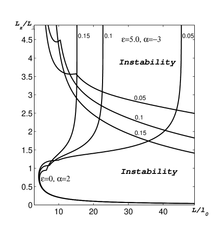
Figure 6: The range of parameters $(L_{z}/L_{\perp};L/l_{0})$ for which the convective shear instability occurs, for $\alpha=2,$ $\,\varepsilon=0$ and $\alpha=-3,$ $\,\varepsilon=5$ for different values of the shear $\lambda=0.05;\,0.1;\,0.15.$

Figures 7 and 8 demonstrate the growth rates of the convective shear instability and the frequencies of the generated convective shear waves for the first $(\alpha=2)$ and the second $(\alpha=-3)$ ranges of the instability. The curves in FIGS. 6-8 have a point $L_{\ast}$ whereby the first derivative $d\gamma_{\rm inst}/dK$ has a singularity. At this point there is a bifurcation which is illustrated in FIGS. 7 and 8. The growth rate of the convective shear instability is determined by the cubic algebraic equation (35). Before the bifurcation point $(L<L_{\ast})$ the cubic equation has three real roots (which corresponds to aperiodic instability). After the bifurcation point $(L>L_{\ast})$ the cubic equation has one real and two complex conjugate roots. When $L>L_{\ast}$ the convective shear waves are generated. When the parameter $L_{z}/L_{\perp}$ increases, the value $L_{\ast}$ decreases. When $L_{z}>L_{\perp},$ the bifurcation point $L_{\ast}<L_{\rm cr}.$ For a given parameter $L/l_{0}$ there are the lower and the upper bounds for the parameter $L_{z}/L_{\perp}$ when the convective shear instability occurs. For large enough parameter $L=L_{u}$ the upper limit of the range of the instability does not exist, e.g., for $\lambda=0.05$ the parameter $L_{u}=47l_{0}$ and for $\lambda=0.15$ the parameter $L_{u}=13l_{0}.$

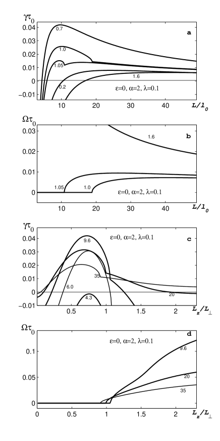
Figure 7: The growth rates of the convective shear instability [a) and c)] and the frequencies of the generated convective shear waves [b) and d)] for the first $(\alpha=2)$ range of the instability and for $\varepsilon=0.$ Corresponding dependencies on the parameter $L/l_{0}$ are given for different $L_{z}/L_{\perp}$ and visa versa.

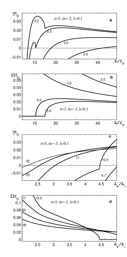
Figure 8: The growth rates of the convective shear instability [a) and c)] and the frequencies of the generated convective shear waves [b) and d)] for the second $(\alpha=-3)$ range of the instability and for $\varepsilon=0.$ Corresponding dependencies on the parameter $L/l_{0}$ are given for different $L_{z}/L_{\perp}$ and visa versa.

Note that when $L<L_{\ast}$ the convective shear waves are not generated and the properties of the convective shear instability are similar to that of the convective wind instability (compare FIG. 2b and the curve for $L/l_{0}=6$ in FIG. 8c). However for $L>L_{\ast}$ these two instabilities are totally different. The properties of the convective shear instability in the first and in the second ranges of the instability are different. In particular, in the second range of the convective shear instability the growth rate monotonically increases, and the frequency of the generated convective shear waves decreases with the parameter $L_{z}/L_{\perp}.$

IV.2 Mechanism of convective shear instability

The mechanism of the convective shear instability associated with the last term in the expression (22) for the turbulent flux of entropy $[{\bf\Phi}\propto\tau_{0}(\mbox{\boldmath$\bar{\omega}$}_{{}_{\parallel}}{\bf\times}{\bf\Phi}^{\ast})]$ is as follows. The vorticity perturbations $\bar{\omega}\equiv(\mbox{\boldmath$\nabla$}{\bf\times}\bar{\bf U})_{z}$ generate perturbations of entropy: $\bar{S}\propto\beta^{-1/6}\,(\tau_{0}/u_{0}){\Phi}^{\ast}_{y}\lambda^{-2/3}\exp(i\pi/6)\bar{\omega}.$ Indeed, consider two vortices (say, ”a” and ”b” in FIG. 9) with the opposite directions of the vorticity $\mbox{\boldmath$\bar{\omega}$}_{{}_{\parallel}}.$ The turbulent flux of entropy is directed towards the boundary between the vortices. The latter increases the mean entropy between the vortices (”a” and ”b”).

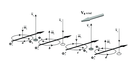
Figure 9: The effect of a nonzero $\mbox{\boldmath$\bar{\omega}$}_{{}_{\parallel}}{\bf\times}{\bf\Phi}^{\ast}$ which causes a redistribution of the horizontal turbulent flux of the entropy. For two vortices (”a” and ”b”) with opposite directions of the vorticity $\mbox{\boldmath$\bar{\omega}$}_{{}_{\parallel}},$ the turbulent flux of entropy is directed towards the boundary between the vortices. The latter increases the mean entropy between the vortices (”a” and ”b”). Similarly, the mean entropy between the vorticies ”b” and ”c” decreases.

Similarly, the mean entropy between the vorticies ”b” and ”c” decreases (see FIG. 9). Such redistribution of the mean entropy causes increase (decrease) of the buoyancy force and formation of upward (downward) flows between the vortices ”a” and ”b” (”b” and ”c”): $\bar{U}_{z}\propto\beta^{1/3}\lambda^{-2/3}g\tau_{0}\,\exp(-i\pi/3)\,\bar{S}.$ Finally, the vertical flows generate vorticity $\bar{\omega}\propto-\beta^{-1/6}\,\lambda^{1/3}\exp(i\pi/6)\bar{U}_{z}/l_{0},$ etc. This results in the excitation of the instability with the growth rate $\gamma_{\rm inst}\propto K^{2/3}$ and generation of the convective shear waves with the frequency $\Omega\propto K^{2/3}\,.$ For perturbations with $K_{x}=0$ the convective shear instability does nor occur. However, for these perturbations with $K_{x}=0$ the convective wind instability can be excited (see Section III), and it is not accompanied by the generation of the convective shear waves. We considered here a linear shear for simplicity. The equilibrium is also possible for a quadratic shear, i.e., when $\bar{\bf U}^{(0)}=\tilde{\lambda}z^{2}{\bf e}_{y}.$

V Discussion

The ”convective wind theory” of turbulent sheared convection is proposed. The developed theory predicts the convective wind instability in a shear-free turbulent convection. This instability causes formation of large-scale semi-organized fluid motions (convective wind) in the form of cells. Spatial characteristics of these motions, such as the minimum size of the growing perturbations and the size of perturbations with the maximum growth rate, are determined.

This study predicts also the existence of the convective shear instability in the sheared turbulent convection. This instability causes formation of large-scale semi-organized fluid motions in the form of rolls (sometimes visualized as the boundary layer cloud streets). These motions can exist in the form of generated convective shear waves, which have a nonzero hydrodynamic helicity. Increase of shear promotes excitation of the convective shear instability.

The proposed here theory of turbulent sheared convection distinguishes between the ”true turbulence”, corresponding to the small-scale part of the spectrum, and the ”convective wind” comprising of large-scale semi-organized motions caused by the inverse energy cascade through large-scale instabilities. The true turbulence in its turn consists of the two parts: the familiar ”Kolmogorov-cascade turbulence” and an essentially anisotropic ”tangling turbulence” caused by tangling of the mean-velocity gradients with the Kolmogorov-type turbulence. These two types of turbulent motions overlap in the maximum-scale part of the spectrum. The tangling turbulence does not exhibit any direct energy cascade.

It was demonstrated here that the characteristic length and time scales of the convective wind motions are much larger than the true-turbulence scales. This justifies separation of scales which is required for the existence of these two types of motions. It is proposed that the term turbulence (or true turbulence) be kept only for the Kolmogorov and tangling turbulence part of the spectrum. This concept implies that the convective wind (as well as semi-organized motions in other very high Reynolds number flows) should not be confused with the true turbulence. The diagram of interactions between turbulent and mean flow objects which cause the large-scale instability and formation of semi-organized structures is shown in FIG. 10.

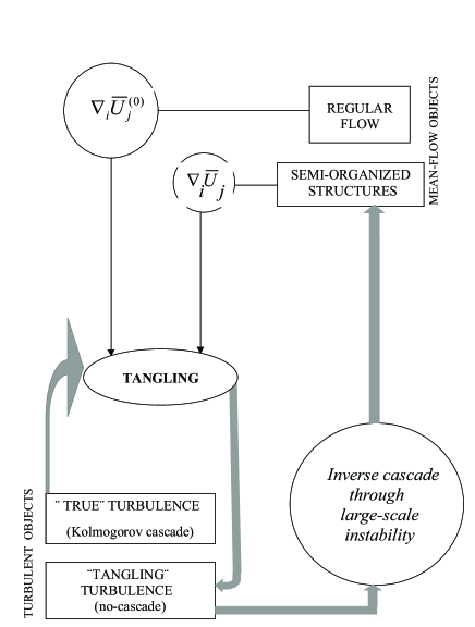
Figure 10: Scheme of interactions between turbulent and mean-flow objects which cause a large-scale instability.

Now let us compare the obtained results with the properties of semi-organized structures observed in the atmospheric convective boundary layer. The semi-organized structures are observed in the form of rolls (cloud streets) or three-dimensional convective cells (cloud cells). Rolls usually align along or at angles of up to $10^{\circ}$ with the mean horizontal wind of the convective layer, with lengths from $20$ to $200$ km, widths from $2$ to $10$ km, and convective depths from $2$ to $3$ km AZ96 . The typical value of the aspect ratio $L_{z}/L_{\perp}\approx 0.14-1.$ The ratio of the minimal size of structures to the maximum scale of turbulent motions is $L/l_{0}=10-100.$ The characteristic life time of rolls varies from $1$ to $72$ hours EB93 . Rolls may occur over both, water surface and land surfaces. The suggested theory predicts the following parameters of the convective rolls: the aspect ratio $L_{z}/L_{\perp}$ ranges from very small to $1,$ and $L/l_{0}=10-100.$ The characteristic time of formation of the rolls $\sim\tau_{0}/\gamma_{\rm inst}$ varies from $1$ to $3$ hours. The life time of the convective rolls is determined by a nonlinear evolution of the convective shear instability. The latter is a subject of a separate ongoing study.

Convective cells may be divided into two types: open and closed. Open-cell circulation has downward motion and clear sky in the cell center, surrounded by cloud associated with upward motion. Closed cells have the opposite circulation AZ96 . Both types of cells have diameters ranging from $10$ to $40$ km and aspect ratios $L_{z}/L_{\perp}\approx 0.05-1,$ and both occur in a convective boundary layer with a depth of about $1$ to $3$ km. The ratio of the minimum size of structures to the maximum scale of turbulent motions is $L/l_{0}=5-20.$ The developed theory predicts the following parameters of the convective cells: the aspect ratio $L_{z}/L_{\perp}$ ranges from very small to $1,$ and $L/l_{0}=5-15.$ The characteristic time of formation of the convective cells $\sim\tau_{0}/\gamma_{\rm inst}$ varies from $1$ to $3$ hours. Therefore the predictions of the developed theory are in a good agreement with observations of the semi-organized structures in the atmospheric convective boundary layer. Moreover, the typical temporal and spatial scales of structures are always much larger then the turbulence scales. This justifies separation of scales which was assumed in the suggested in the theory.

Appendix A Derivations of expressions for the Reynolds stresses and turbulent flux of entropy

Equations (2) and (3) yield the following conservation equations for the kinetic energy $W_{v}=\rho_{0}{\bf v}^{2}/2,$ for $W_{S}=\rho_{0}S^{2}/2$ and for ${\bf W}^{\Phi}=\rho_{0}S{\bf v}:$

$${\partial W_{v}\over\partial t}+\mbox{\boldmath$\nabla$}\cdot{\bf F}_{v} = I_{v}-D_{v}\;,$$ (39)

$${\partial W_{S}\over\partial t}+\mbox{\boldmath$\nabla$}\cdot{\bf F}_{S} = I_{S}-D_{S}\;,$$ (40)

$${\partial W_{i}^{\Phi}\over\partial t}+\mbox{\boldmath$\nabla$}_{j}{\bf F}_{ij}^{\Phi} = I_{i}^{\Phi}-D_{i}^{\Phi}\;,$$ (41)

where $I_{v}=-\rho_{0}({\bf v}\cdot{\bf g})S,$ $\,I_{S}=-I_{v}\Omega_{b}^{2}/g^{2},$ and ${\bf I}^{\Phi}=-\rho_{0}[{\bf v}({\bf v}~{}\cdot~{}{\bf N}_{b})+S^{2}{\bf g}]+(P/\rho_{0})\mbox{\boldmath$\nabla$}(S\rho_{0})$ are the source terms in these equations, $D_{v}=-\rho_{0}({\bf v}\cdot{\bf f}_{\nu}),$ $\,D_{S}=\rho_{0}S\,(\mbox{\boldmath$\nabla$}\cdot{\bf F}_{\kappa})$ and ${\bf D}^{\Phi}=-\rho_{0}S{\bf f}_{\nu}+(\rho_{0}/T_{0}){\bf v}(\mbox{\boldmath$\nabla$}\cdot{\bf F}_{\kappa})$ are the dissipative terms, ${\bf F}_{v}={\bf v}\,(W_{v}+P),$ $\,{\bf F}_{S}={\bf v}W_{S}$ and ${\bf F}_{ij}^{\Phi}=\rho_{0}Sv_{i}v_{j}+SP\delta_{ij}$ are the fluxes. Equations (39) and (40) yield conservation equation for $W_{E}=W_{v}\Omega_{b}^{2}/g^{2}+W_{S}$

$${\partial W_{E}\over\partial t}+\mbox{\boldmath$\nabla$}\cdot{\bf F}_{E} = -D_{E}\;,$$ (42)

where $D_{E}=D_{v}\Omega_{b}^{2}/g^{2}+D_{S}$ is the dissipative term, and ${\bf F}_{E}={\bf F}_{v}\Omega_{b}^{2}/g^{2}+{\bf F}_{S}$ is the flux. Equation (42) does not have a source term, and this implies that without dissipation $(D_{E}=0)$ the value $\int W_{E}\,dV$ is conserved, where in the latter formula the integration is performed over the volume. For the convection $\Omega_{b}^{2}<0$ and, therefore, $W_{S}\approx W_{v}|\Omega_{b}^{2}|/g^{2}.$

Using Eqs. (39)-(41) we derived balance equations for the second moments. In particular, averaging Eqs. (39)-(41) over the ensemble of fluctuations and subtracting from these equations the corresponding equations for the mean fields: $\rho_{0}\bar{\bf U}^{2}/2,$ $\,\rho_{0}\bar{S}^{2}/2,$ $\,\rho_{0}\bar{S}\bar{\bf U},$ yields

$$\biggl{(}{\partial\over\partial t} + \bar{\bf U}\cdot\mbox{\boldmath$\nabla$}\biggr{)}f_{pp}+2f_{ij}\nabla_{j}\bar{U}_{i}+2{\bf\Phi}{\bf\cdot}{\bf g}+{2\over\rho_{0}}\mbox{\boldmath$\nabla$}\cdot{\bf\Psi}_{E}$$ (43)

$$=-{f_{\ast}\over\tau_{0}\delta_{\ast}}\biggl{(}1+{\varepsilon\over 2}\biggr{)}\;,$$

$$\biggl{(}{\partial\over\partial t} + \bar{\bf U}\cdot\mbox{\boldmath$\nabla$}\biggr{)}\Phi_{i}+({\bf\Phi}\cdot\mbox{\boldmath$\nabla$})\bar{U}_{i}+f_{ij}({\bf N_{b}}+\mbox{\boldmath$\nabla$}\bar{S})_{j}$$ (44)

$$-{1\over 2}ge_{i}(4-\gamma)H+{1\over\rho_{0}}\nabla_{j}\Psi_{ij}-\biggl{(}{\gamma P_{0}\over\rho_{0}}\biggr{)}H({\bf N_{b}})_{i}$$

$$=-{\Phi^{\ast}_{i}\over 2\tau_{0}\delta_{\ast}}(1+{\rm Pr})\;,$$

$$\biggl{(}{\partial\over\partial t} + \bar{\bf U}\cdot\mbox{\boldmath$\nabla$}\biggr{)}H+2\Phi_{j}({\bf N_{b}}+\mbox{\boldmath$\nabla$}\bar{S})_{j}=-{H_{\ast}\over\tau_{0}\delta_{\ast}}\;,$$ (45)

where ${\rm Pr}=\nu/\kappa$ is the Prandtl number, $\nu$ is the kinematic viscosity, ${\bf\Psi}_{E}=\rho_{0}f_{pp}{\bf u}/2+\langle p{\bf u}\rangle,$ $\,\Psi_{ij}=\rho_{0}\langle su_{i}u_{j}\rangle+\delta_{ij}(\gamma P_{0}H/2+\langle sp\rangle),$ and we took into account that the dissipations of energy, the flux of entropy and the second moment of entropy $H$ are determined by the background turbulent convection described by Eqs. (12)-(17). In derivation of Eq. (44) we used an identity $\rho_{0}S\mbox{\boldmath$\nabla$}(P/\rho_{0})\simeq\mbox{\boldmath$\nabla$}(\gamma P_{0}S^{2})/2+\gamma P_{0}S^{2}{\bf N_{b}}+(\gamma/2-1)\rho_{0}{\bf g}S^{2},$ and we assumed that $S\simeq P/\gamma P_{0},$ i.e., we neglected fluctuations of density $\rho/\rho_{0}.$ Equations (43)-(45) allow us to determine $f_{\ast},$ $\,{\bf\Phi}^{\ast}$ and $\,H_{\ast}$ in the background turbulent convection (see below).

Using Eqs. (6) and (7) we derived equations for the following second moments:

$$f_{ij}({\bf k},{\bf R}) = \langle u_{i}({\bf k},{\bf R})u_{j}(-{\bf k},{\bf R})\rangle\;,$$ (46)

$$\Phi_{i}({\bf k},{\bf R}) = \langle s({\bf k},{\bf R})u_{i}(-{\bf k},{\bf R})\rangle\;,$$ (47)

$$F({\bf k},{\bf R}) = \langle s({\bf k},{\bf R})\omega(-{\bf k},{\bf R})\rangle\;,$$ (48)

$$G({\bf k},{\bf R}) = \langle\omega({\bf k},{\bf R})\omega(-{\bf k},{\bf R})\rangle\;,$$ (49)

$$H({\bf k},{\bf R}) = \langle s({\bf k},{\bf R})s(-{\bf k},{\bf R})\rangle\;,$$ (50)

where $\omega\equiv(\mbox{\boldmath$\nabla$}{\bf\times}{\bf u})_{z}$ and we use a two-scale approach, , i.e., a correlation function is written as follows

$$\langle u_{i}({\bf x})u_{j}({\bf y})\rangle = \int\langle u_{i}({\bf k}_{1})u_{j}({\bf k}_{2})\rangle\exp[i({\bf k}_{1}{\bf\cdot}{\bf x}$$

$$+{\bf k}_{2}{\bf\cdot}{\bf y})]\,d{\bf k}_{1}\,d{\bf k}_{2}$$

$$= \int f_{ij}({\bf k,R})\exp(i{\bf k}{\bf\cdot}{\bf r})\,d{\bf k}\;,$$

$$f_{ij}({\bf k,R}) = \int\langle u_{i}({\bf k}+{\bf K}/2)u_{j}(-{\bf k}+{\bf K}/2)\rangle$$

$$\times\exp(i{\bf K}{\bf\cdot}{\bf R})\,d{\bf K}\;$$

(see, e.g., RS75 ; KR94 ), where ${\bf R}$ and ${\bf K}$ correspond to the large scales, and ${\bf r}$ and ${\bf k}$ to the small scales, i.e., ${\bf R}=({\bf x}+{\bf y})/2,$ $\quad{\bf r}={\bf x}-{\bf y},$ $\quad{\bf K}={\bf k}_{1}+{\bf k}_{2},$ $\quad{\bf k}=({\bf k}_{1}-{\bf k}_{2})/2.$ This implies that we assumed that there exists a separation of scales, i.e., the maximum scale of turbulent motions $l_{0}$ is much smaller then the characteristic scale $L$ of inhomogeneities of the mean fields. In particular, this implies that $r\leq l_{0}\ll R.$ Our final results showed that this assumption is indeed valid. Now let us calculate

$${\partial f_{ij}({\bf k}_{1},{\bf k}_{2})\over\partial t} \equiv \langle P_{in}({\bf k}_{1}){\partial u_{n}({\bf k}_{1})\over\partial t}u_{j}({\bf k}_{2})\rangle$$ (51)

$$+\langle u_{i}({\bf k}_{1})P_{jn}({\bf k}_{2}){\partial u_{n}({\bf k}_{2})\over\partial t}\rangle\;,$$

$${\partial\Phi_{j}({\bf k}_{1},{\bf k}_{2})\over\partial t} \equiv \langle s({\bf k}_{1})P_{jn}({\bf k}_{2}){\partial u_{n}({\bf k}_{2})\over\partial t}\rangle$$ (52)

$$+\langle{\partial s({\bf k}_{1})\over\partial t}u_{j}({\bf k}_{2})\rangle\;,$$

where we multiplied equation of motion (6) rewritten in ${\bf k}$-space by $P_{ij}({\bf k})=\delta_{ij}-k_{ij}$ in order to exclude the pressure term from the equation of motion.

Thus, equations for $f_{ij}({\bf k,R})$ and ${\bf\Phi}({\bf k,R})$ read:

$${\partial f_{ij}({\bf k})\over\partial t} = \hat{I}_{ijmn}f_{mn}({\bf k})+N_{ij}({\bf k})\;,$$ (53)

$${\partial\Phi_{i}({\bf k})\over\partial t} = \hat{I}_{ij}\Phi_{j}({\bf k})+M_{i}({\bf k})\;,$$ (54)

where

$$\hat{I}_{ijmn} = 2(k_{iq}\delta_{mp}\delta_{jn}+k_{jq}\delta_{im}\delta_{pn})\nabla_{p}\bar{U}_{q}-\biggl{(}\delta_{im}\delta_{jq}\delta_{np}$$ (55)

$$+\delta_{iq}\delta_{jn}\delta_{mp}-\delta_{im}\delta_{jn}k_{q}{\partial\over\partial k_{p}}\biggr{)}\nabla_{p}\bar{U}_{q}\;,$$

$$\hat{I}_{ij} = 2k_{in}\nabla_{j}\bar{U}_{n}+\delta_{ij}k_{n}{\partial\over\partial k_{m}}\nabla_{m}\bar{U}_{n}-\nabla_{j}\bar{U}_{i}\;,$$ (56)

$$N_{ij}({\bf k}) = ge_{m}[P_{im}({\bf k})\Phi_{j}({\bf k})+P_{jm}({\bf k})\Phi_{i}(-{\bf k})]$$ (57)

$$+f_{ij}^{N}({\bf k})\;,$$

$$M_{i}({\bf k}) = -f_{mi}({\bf N_{b}}+\mbox{\boldmath$\nabla$}\bar{S})_{m}+ge_{m}P_{im}({\bf k})H$$ (58)

$$+\Phi_{i}^{N}\;,$$

and hereafter we consider the case with $\mbox{\boldmath$\nabla$}\cdot\bar{\bf U}=0$ (i.e., $\Lambda=0).$ Here $f_{ij}^{N}$ and $\Phi_{i}^{N}$ are the third moments appearing due to the nonlinear terms. Equations (53) and (54) are written in a frame moving with a local velocity $\bar{\bf U}$ of the mean flow. In Eqs. (53)-(58) we neglected small terms which are of the order of $O(\nabla^{3}\bar{\bf U})$ and $O(\nabla^{2}f_{ij};\nabla^{2}\Phi_{i}).$ Note that Eqs. (53)-(58) do not contain the terms proportional to $O(\nabla^{2}\bar{\bf U}).$ The first term in the RHS of Eqs. (53) and (54) depends on the gradients of the mean fluid velocity $(\nabla_{i}\bar{U}_{j}).$ Equations for the second moments $G({\bf k}),$ $\,F({\bf k})$ and $H({\bf k})$ read:

$${\partial G({\bf k})\over\partial t} = ({\bf e}{\bf\times}\tilde{\bf k}_{1})_{i}({\bf e}{\bf\times}\tilde{\bf k}_{2})_{j}\,{\partial f_{ij}({\bf k})\over\partial t}\;,$$ (59)

$${\partial F({\bf k})\over\partial t} = -i({\bf e}{\bf\times}\tilde{\bf k}_{1})_{j}\,{\partial\Phi_{j}({\bf k})\over\partial t}\;,$$ (60)

$${\partial H({\bf k})\over\partial t} = Q({\bf k})\;,$$ (61)

where $Q({\bf k})=-2{\bf\Phi}({\bf k})\cdot({\bf N}_{b}+\mbox{\boldmath$\nabla$}\bar{S})+H_{N},$ and $H_{N}$ is the third moment appearing due to the nonlinear terms, $\tilde{\bf k}_{1}={\bf k}-(i/2)\mbox{\boldmath$\nabla$},$ $\,\tilde{\bf k}_{2}={\bf k}+(i/2)\mbox{\boldmath$\nabla$}.$ The terms $\sim{\bf\Phi}$ in the tensor $N_{ij}({\bf k})$ [see Eqs. (53) and (57)] can be considered as a stirring force for the turbulent convection. On the other hand, the terms $\sim({\bf N}_{b}+\mbox{\boldmath$\nabla$}\bar{S})$ in Eqs. (54), (58) and (61) are the sources of the flux of entropy ${\bf\Phi}$ and the second moment of entropy $H.$ Note that a stirring force in the Navier-Stokes turbulence is an external parameter.

Since the equations for the second moments contain the third moments, a problem of closure for the higher moments arises. In this study we used the $\tau$ approximation [see Eq. (11)] which allows us to express the third moments $f^{N}_{ij},$ ${\bf\Phi}^{N}$ and $H_{N}$ in Eqs. (53), (54) and (61) in terms of the second moments. Here we define a background turbulent convection as the turbulent convection with zero gradients of the mean fluid velocity $(\nabla_{i}\bar{U}_{j}=0)].$ The background turbulent convection is determined by the following equations:

$${\partial f_{ij}^{(0)}({\bf k})\over\partial t} = N_{ij}^{(0)}({\bf k})\;,$$ (62)

$${\partial\Phi_{i}^{(0)}({\bf k})\over\partial t} = M_{i}^{(0)}({\bf k})\;,$$ (63)

$${\partial H^{(0)}({\bf k})\over\partial t} = Q^{(0)}({\bf k})\;.$$ (64)

A nonzero gradient of the mean fluid velocity results in deviations from the background turbulent convection. These deviations are determined by the following equations:

$${\partial(f_{ij}-f_{ij}^{(0)})\over\partial t} = \hat{I}_{ijmn}\,f_{mn}({\bf k})-{f_{ij}-f_{ij}^{(0)}\over\tau(k)}\;,$$ (65)

$${\partial(\Phi_{i}-\Phi_{i}^{(0)})\over\partial t} = \hat{I}_{ij}\,\Phi_{j}({\bf k})-{\Phi_{i}-\Phi_{i}^{(0)}\over\tau(k)}\;,$$ (66)

$${\partial(H-H^{(0)})\over\partial t} = -{H-H^{(0)}\over\tau(k)}\;,$$ (67)

where the deviations (caused by a nonzero gradients of the mean fluid velocity) of the functions $N_{ij}({\bf k})-N_{ij}^{(0)}({\bf k})$ and $M_{i}({\bf k})-M_{i}^{(0)}({\bf k})$ from the background state are described by the relaxation terms: $-(f_{ij}-f_{ij}^{(0)})/\tau(k)$ and $-(\Phi_{i}-\Phi_{i}^{(0)})/\tau(k),$ respectively. Similarly, the deviation $Q({\bf k})-Q^{(0)}({\bf k})$ is described by the term $-(H-H^{(0)})/\tau(k).$ Here we assumed that the correlation time $\tau(k)$ is independent of the gradients of the mean fluid velocity.

Now we assume that the characteristic times of variation of the second moments $f_{ij}({\bf k}),$ $\Phi_{i}({\bf k})$ and $H({\bf k})$ are substantially larger than the correlation time $\tau(k)$ for all turbulence scales. This allows us to determine a stationary solution for the second moments $f_{ij}({\bf k}),$ $\Phi_{i}({\bf k})$ and $H({\bf k}):$

$$f_{ij}({\bf k}) = f_{ij}^{(0)}({\bf k})+\tau(k)\hat{I}_{ijmn}\,f_{mn}^{(0)}({\bf k})\;,$$ (68)

$$\Phi_{i}({\bf k}) = \Phi_{i}^{(0)}({\bf k})+\tau(k)\hat{I}_{ij}\,\Phi_{j}^{(0)}({\bf k})\;,$$ (69)

$$H({\bf k}) = H^{(0)}({\bf k})\;,$$ (70)

where we neglected the third and higher order spatial derivatives of the mean velocity field $\bar{\bf U}.$

For the integration in ${\bf k}$-space of the second moments $f_{ij}({\bf k}),$ $\Phi_{i}({\bf k}),\ldots,$ $H({\bf k},{\bf R})$ we have to specify a model for the background turbulent convection. We used the model of the background turbulent convection determined by Eqs. (12)-(17). For the integration in ${\bf k}$-space we used identities given in Appendix C. The integration in ${\bf k}$-space of Eqs. (68) and (69) yields the following equations for the Reynolds stresses and the turbulent flux of entropy:

$$f_{ij} = f_{ij}^{(0)}-\nu_{T}\biggl{(}a_{1}\,(\nabla_{i}\bar{U}_{j}+\nabla_{j}\bar{U}_{i})+a_{2}\,(e_{i}\nabla_{j}$$ (71)

$$+e_{j}\nabla_{i})\bar{U}_{z}-c_{2}\,{\partial\over\partial z}(e_{i}\bar{U}_{j}+e_{j}\bar{U}_{i})$$

$$+{\partial\bar{U}_{z}\over\partial z}(c_{3}\,e_{ij}+a_{3}\,\delta_{ij})\biggr{)}\;,$$

$${\bf\Phi} = {\bf\Phi}^{\ast}+{\tau_{0}\over 30}({\bf\Phi}^{\ast}\cdot{\bf e})\biggl{(}{\partial\over\partial z}(b_{1}\,\bar{U}_{z}{\bf e}+b_{2}\,\bar{\bf U})-b_{3}\,\mbox{\boldmath$\nabla$}^{\perp}\bar{U}_{z}\biggr{)}$$ (72)

$$-{\tau_{0}\over 5}\biggl{[}2({\bf\Phi}^{\ast}{\bf\times}{\bf e})\bar{\omega}+5({\bf\Phi}^{\ast}\cdot\mbox{\boldmath$\nabla$})\bar{\bf U}-2({\bf\Phi}^{\ast}\cdot\mbox{\boldmath$\nabla$}_{\perp})\bar{\bf U}$$

$$+(3-q)({\bf e}{\bf\times}\mbox{\boldmath$\nabla$})({\bf\Phi}^{\ast}\cdot({\bf e}{\bf\times}\bar{\bf U}))$$

$$-(q-1)[(({\bf\Phi}^{\ast}{\bf\times}{\bf e})\cdot\mbox{\boldmath$\nabla$})({\bf e}{\bf\times}\bar{\bf U})\biggr{]}\,,$$

where $\nu_{T}=\tau_{0}f_{\ast}/6,$ $\,\bar{\omega}=(\mbox{\boldmath$\nabla$}{\bf\times}\bar{\bf U})_{z},$ $\,a_{1}=c_{1}+c_{2},$ $\,a_{2}=-\varepsilon(q-1)/4,$ $\,a_{3}=-\varepsilon(5-q)/4,$ $\,b_{1}=(8\alpha-3)(q+1),$ $\,b_{2}=3(9-q)-2\alpha(q+1),$ $\,b_{3}=(2\alpha+3)(q+1),$ $\,c_{1}=(q+3)/5,$ $\,c_{2}=\varepsilon(q+1)/4,$ $\,c_{3}=\varepsilon(q+3)/4.$

Equations (71) and (72) imply that there are two contributions to the Reynolds stresses and turbulent flux of entropy which correspond to two kinds of fluctuations of the velocity field. The first contribution is due to the Kolmogorov turbulence with the spectrum $(\propto k^{-q}),$ and it corresponds to the background turbulent convection. The second kind of fluctuations depends on gradients of the mean velocity field and is caused by a ”tangling” of gradients of the mean velocity field by turbulent motions. The spectrum of the tangling turbulence is $W(k)\tau(k)\propto k^{1-2q}$ [see Eqs. (68) and (69)]. These fluctuations describe deviations from the background turbulent convection caused by the gradients of the mean fluid velocity field.

Now we calculate a dissipation of the kinetic energy of the mean flow $\bar{\bf U}:$

$$D_{U}\equiv-(1/2)(f_{ij}-f_{ij}^{(0)})(\nabla_{i}\bar{U}_{j}+\nabla_{j}\bar{U}_{i})\;,$$ (73)

using a general form of the velocity field $\bar{U}_{i}=\bar{V}_{i}(t,{\bf K})\exp(i{\bf K}\cdot{\bf R}),$ where

$$\bar{V}_{i}(t,{\bf K}) = \biggl{(}{K\over K_{\perp}}\biggr{)}^{2}[P_{ij}({\bf K})e_{j}\bar{V}_{z}(t,{\bf K})$$ (74)

$$-iK^{-2}({\bf e}{\bf\times}{\bf K})_{i}\,\tilde{\omega}(t,{\bf K})]\;,$$

and $\tilde{\omega}=(\mbox{\boldmath$\nabla$}{\bf\times}\bar{\bf V})_{z}.$ The result is given by

$$D_{U}(t,{\bf K}) = \nu_{T}\biggl{\{}b_{4}\,\biggl{(}{K\over K_{\perp}}\biggr{)}^{2}[K^{2}\bar{V}_{z}^{2}(t,{\bf K})+\tilde{\omega}^{2}(t,{\bf K})]$$ (75)

$$+b_{5}\,K^{2}\bar{V}_{z}^{2}(t,{\bf K})\biggr{\}}\;,$$

where $b_{4}=c_{1}+c_{2}\sin^{2}\theta$ and $b_{5}=a_{2}+c_{3}\cos^{2}\theta.$ The function $D_{U}(t,{\bf K})$ must be positive for statistically stationary small-scale turbulence. The latter is valid when $\varepsilon$ satisfies condition (21).

Appendix B The model of the background turbulent convection

A simple approximate model for the three-dimensional isotropic Navier-Stokes turbulence is described by a two-point correlation function of the velocity field $f_{ij}(t,{\bf x},{\bf y})=\langle u_{i}(t,{\bf x})u_{j}(t,{\bf y})\rangle$ with the Kolmogorov spectrum $W(k)\propto k^{-q}$ and $q=5/3.$ The turbulent convection is determined not only by the turbulent velocity field ${\bf u}(t,{\bf x})$ but by the fluctuations of the entropy $s(t,{\bf x}).$ This implies that for the description of the turbulent convection one needs additional correlation functions, e.g., the turbulent flux of entropy ${\bf\Phi}_{i}(t,{\bf x},{\bf y})=\langle s(t,{\bf x})u_{i}(t,{\bf y})\rangle$ and the second moment of the entropy fluctuations $H(t,{\bf x},{\bf y})=\langle s(t,{\bf x})s(t,{\bf y})\rangle.$ Note also that the turbulent convection is anisotropic.

Let us derive Eqs. (12) and (13) for the correlation functions $f_{ij}$ and ${\bf\Phi}_{i}.$ To this end, the velocity ${\bf u}_{\perp}$ is written as a sum of the vortical and the potential components, i.e., ${\bf u}_{\perp}=\mbox{\boldmath$\nabla$}{\bf\times}(\tilde{C}{\bf e})+\mbox{\boldmath$\nabla$}_{\perp}\tilde{\phi},$ where $\omega\equiv(\mbox{\boldmath$\nabla$}{\bf\times}{\bf u})_{z}=-\Delta_{\perp}\tilde{C},$ $\,\Delta_{\perp}\tilde{\phi}=-\partial u_{z}/\partial z,$ $\,\mbox{\boldmath$\nabla$}_{\perp}=\mbox{\boldmath$\nabla$}-{\bf e}({\bf e}\cdot\mbox{\boldmath$\nabla$}).$ Hereafter $\Lambda=0.$ Thus, in ${\bf k}$-space the velocity ${\bf u}$ is given by

$$u_{i}({\bf k}) = (k/k_{\perp})^{2}[e_{m}P_{im}({\bf k})u_{z}({\bf k})-i({\bf e}{\bf\times}{\bf k})_{i}\omega({\bf k})/k^{2}].$$

Multiplying Eq. (LABEL:C80) for $u_{i}({\bf k}_{1})$ by $u_{j}({\bf k}_{2})$ and averaging over the turbulent velocity field we obtain

$$f_{ij}^{(0)}({\bf k}) = (k/k_{\perp})^{4}[f_{\ast}f^{(0)}({\bf k})e_{mn}P_{im}({\bf k})P_{jn}({\bf k})$$ (77)

$$+({\bf e}{\bf\times}{\bf k})_{i}({\bf e}{\bf\times}{\bf k})_{j}G^{(0)}({\bf k})/k^{4}]\;,$$

where we assumed that the turbulent velocity field in the background turbulent convection is non-helical. Now we use an identity

$$(k/k_{\perp})^{2}e_{mn}P_{im}({\bf k})P_{jn}({\bf k})=e_{ij}+k_{ij}^{\perp}-k_{ij}$$

$$=P_{ij}({\bf k})-P_{ij}^{\perp}({\bf k}_{\perp})\;,$$ (78)

which can be derived from

$$k_{z}(k_{z}e_{ij}+e_{i}k_{j}^{\perp}+e_{j}k_{i}^{\perp})=k_{ij}k^{2}-k_{ij}^{\perp}k_{\perp}^{2}\;.$$

Here we also used the identity $({\bf k}_{\perp}{\bf\times}{\bf e})_{i}({\bf k}_{\perp}{\bf\times}{\bf e})_{j}=k_{\perp}^{2}P_{ij}^{(\perp)}(k_{\perp}).$ Substituting Eq. (78) into Eq. (77) we obtain

$$f_{ij}^{(0)}({\bf k}) = (k/k_{\perp})^{2}\{f_{\ast}f^{(0)}({\bf k})P_{ij}({\bf k})+[G^{(0)}({\bf k})/k^{2}$$ (79)

$$-f_{\ast}f^{(0)}({\bf k})]P_{ij}^{\perp}({\bf k}_{\perp})\}\;.$$

Thus two independent functions determine the correlation function of the anisotropic turbulent velocity field. In the isotropic three-dimensional turbulent flow $G^{(0)}({\bf k})/k^{2}=f_{\ast}f^{(0)}({\bf k})$ and the correlation function reads

$$f_{ij}^{(0)}({\bf k})=f_{\ast}W(k)P_{ij}({\bf k})/8\pi k^{2}\;.$$ (80)

In the isotropic two-dimensional turbulent flow $G^{(0)}({\bf k})/k^{2}\gg f_{\ast}f^{(0)}({\bf k})$ and the correlation function is given by

$$f_{ij}^{(0)}({\bf k})=G^{(0)}({\bf k})P_{ij}^{\perp}({\bf k}_{\perp})/k_{\perp}^{2}\;.$$ (81)

A simplest generalization of these correlation functions is an assumption that $G^{(0)}({\bf k})/[k^{2}f_{\ast}f^{(0)}({\bf k})]-1=\varepsilon=const,$ and thus the correlation function $f_{ij}^{(0)}({\bf k})$ is given by Eq. (12). This correlation function can be considered as a combination of Eqs. (80) and (81) for the three-dimensional and two-dimensional turbulence. When $\varepsilon$ depends on the wave vector ${\bf k},$ the correlation function $f_{ij}^{(0)}({\bf k})$ is determined by two spectral functions.

Now we derive Eq. (13) for the turbulent flux of entropy. Multiplying Eq. (LABEL:C80) written for $u_{i}({\bf k}_{2})$ by $s({\bf k}_{1})$ and averaging over turbulent velocity field we obtain Eq. (13). Multiplying Eq. (13) by $i({\bf k}_{\perp}{\bf\times}{\bf e})_{i}$ we get

$$F^{(0)}({\bf k})=i({\bf k}_{\perp}{\bf\times}{\bf e})\cdot{\bf\Phi}_{\perp}^{(0)}({\bf k})\;.$$ (82)

Now we assume that ${\bf\Phi}_{\perp}^{(0)}({\bf k})\propto{\bf\Phi}^{\ast}_{\perp}f^{(0)}({\bf k}).$ The integration in ${\bf k}$-space in Eq. (82) yields the numerical factor in Eq. (15). Note that for simplicity we assumed that the correlation functions $F^{(0)}({\bf k})$ and $f^{(0)}({\bf k})$ have the same spectrum. If these functions have different spectra, it results only in a different value of a numerical coefficient in Eq. (15).

Now let us discuss the physical meaning of the parameter $\alpha.$ To this end we derived the equation for the two-point correlation function $\Phi_{z}^{(0)}({\bf r})=\langle s({\bf x})\,{\bf u}({\bf x}+{\bf r})\rangle$ of the turbulent flux of entropy for the background turbulent convection (which corresponds to Eq. (14) written in ${\bf k}$-space). Let us we rewrite Eq. (14) in the following form:

$$\Phi_{z}^{(0)}({\bf k}) = ({\bf\Phi}^{\ast}\cdot{\bf e})[k^{2}+\Gamma({\bf e}\cdot{\bf k})^{2}]\tilde{\Phi}_{w}(k)\;,$$ (83)

$$\tilde{\Phi}_{w}(k) = -(3-\alpha)W(k)/8\pi k^{4}\;,$$ (84)

where $\Gamma=3(\alpha-1)/(3-\alpha).$ The Fourier transform of Eq. (83) reads

$$\Phi_{z}^{(0)}({\bf r}) = ({\bf\Phi}^{\ast}\cdot{\bf e})[\Delta+\Gamma({\bf e}\cdot\mbox{\boldmath$\nabla$})^{2}]\Phi_{w}(r)\;,$$ (85)

where $\Phi_{w}(r)$ is the Fourier transform of the function $\tilde{\Phi}_{w}(k).$ Now we use the identity

$$\nabla_{i}\nabla_{j}\Phi_{w}(r)=\psi(r)\,\delta_{ij}+r\psi^{\prime}(r)\,r_{ij}\;,$$ (86)

where $\psi(r)=r^{-1}\Phi^{\prime}_{w}(r)$ and $\psi^{\prime}(r)=d\psi/dr.$ Equations (85) and (86) yield the two-point correlation function $\Phi_{z}^{(0)}({\bf r}):$

$$\Phi_{z}^{(0)}({\bf r}) = ({\bf\Phi}^{\ast}\cdot{\bf e})\biggl{(}\psi(r)$$ (87)

$$+r\psi^{\prime}(r){1+\Gamma\cos^{2}\tilde{\theta}\over 3+\Gamma}\biggr{)}\;,$$

where $\tilde{\theta}$ is the angle between ${\bf e}$ and ${\bf r}.$ The function $\psi(r)$ has the following properties: $\psi(r=0)=1$ and $(r\psi^{\prime})_{r=0}=0,$ e.g., the function $\psi(r)=1-(r/l_{0})^{q-1}$ satisfies the above properties, where $1<q<3.$ Thus, the two-point correlation function $\Phi_{z}^{(0)}({\bf r})$ of the flux of entropy for the background turbulent convection is given by

$$\Phi_{z}^{(0)}({\bf r}) = ({\bf\Phi}^{\ast}\cdot{\bf e})\biggl{[}1-\biggl{(}{(q-1)(1+\Gamma\cos^{2}\tilde{\theta})\over 3+\Gamma}$$ (88)

$$+1\biggr{)}\biggl{(}{r\over l_{0}}\biggr{)}^{q-1}\biggr{]}\;.$$

Simple analysis shows that $-3/(q-1)<\alpha<3,$ where we took into account that $\partial\Phi_{z}^{(0)}({\bf r})/\partial r<0$ for all angles $\tilde{\theta}.$ The parameter $\alpha$ can be presented as $\alpha=[1+\xi(q+1)/(q-1)]/(1+\xi/3)$ and $\xi=(l_{\perp}/l_{z})^{q-1}-1,$ where $l_{\perp}$ and $l_{z}$ are the horizontal $(\tilde{\theta}=\pi/2)$ and the vertical $(\tilde{\theta}=0)$ scales in which the correlation function $\Phi_{z}^{(0)}({\bf r})$ tends to zero. The parameter $\xi$ describes the degree of thermal anisotropy. In particular, when $l_{\perp}=l_{z}$ the parameter $\xi=0$ and $\alpha=1.$ For $l_{\perp}\ll l_{z}$ the parameter $\xi=-1$ and $\alpha=-3/(q-1).$ The maximum value $\xi_{\rm max}$ of the parameter $\xi$ is given by $\xi_{\rm max}=q-1$ for $\alpha=3.$ Thus, for $\alpha<1$ the thermal structures have the form of column or thermal jets $(l_{\perp}<l_{z}),$ and $\alpha>1$ there exist the ‘’pancake” thermal structures $(l_{\perp}>l_{z})$ in the background turbulent convection.

Appendix C The identities used for the integration in ${\bf k}$-space

To integrate over the angles in ${\bf k}$-space of Eqs. (68) and (69) we used the following identities:

$$\int k_{ijmn}\,d\hat{\Omega}=(4\pi/15)\Delta_{ijmn}\;,$$

$$\int k_{ij}\sin^{2}\theta\,d\hat{\Omega}=(8\pi/15)(2\delta_{ij}-e_{ij})\;,$$

$$\int k_{ijmn}\sin^{2}\theta\,d\hat{\Omega}=(8\pi/105)(3\Delta_{ijmn}-\Gamma_{ijmn})\;,$$

$$\int k_{ij}^{\perp}\,d\hat{\Omega}=2\pi P_{ij}({\bf e})\;,$$

$$\int k_{ij}^{\perp}k_{mn}\,d\hat{\Omega}=(\pi/3)[P_{ij}({\bf e})(\delta_{mn}+e_{mn})$$

$$+P_{in}({\bf e})P_{mj}({\bf e})+P_{im}({\bf e})P_{nj}({\bf e})]\;,$$

$$e_{j}\int k_{i}^{\perp}k_{j}k_{mn}k_{\perp}^{-2}\,d\hat{\Omega}=(2\pi/3)[P_{in}({\bf e})e_{m}+P_{im}({\bf e})e_{n}]\;,$$

$$e_{j}\int k_{i}^{\perp}k_{j}k_{mn}k^{-2}\,d\hat{\Omega}=(4\pi/3)[P_{in}({\bf e})e_{m}+P_{im}({\bf e})e_{n}]\;,$$

where $P_{ij}({\bf e})=\delta_{ij}-e_{ij},$ $\,k_{ijmn}=k_{i}k_{j}k_{m}k_{n}/k^{4},$ $\,d\hat{\Omega}=\sin\theta\,d\theta\,d\varphi,$ and

$$\Delta_{ijmn} = \delta_{ij}\delta_{mn}+\delta_{im}\delta_{nj}+\delta_{in}\delta_{mj}\;,$$

$$\Gamma_{ijmn} = \delta_{ij}e_{mn}+\delta_{im}e_{jn}+\delta_{in}e_{jm}+\delta_{jm}e_{in}$$

$$+\delta_{jn}e_{im}+\delta_{mn}e_{ij}\;,$$

$$\gamma_{ijm} = \Delta_{ijmn}e_{n}=\delta_{ij}e_{m}+\delta_{im}e_{j}+\delta_{jm}e_{i}\;,$$

$$e_{m}\gamma_{ijm} = \delta_{ij}+2e_{ij}\;,$$

$$e_{n}\Gamma_{ijmn} = \gamma_{ijm}+3e_{ijm}\;,\quad e_{mn}\Gamma_{ijmn}=\delta_{ij}+5e_{ij}\;,$$

$$P_{ij}({\bf k}) + \varepsilon P_{ij}^{\perp}({\bf k}_{\perp})=(1+\varepsilon)\delta_{ij}-\varepsilon e_{ij}-k_{ij}-\varepsilon k_{ij}^{\perp}\;.$$

The above identities allow us to calculate the following integrals (which were used for the derivation of equations for the Reynolds stresses and turbulent flux of entropy):

$$\int\tau(k)k_{ij}\Phi_{m}^{(0)}({\bf k})\,d{\bf k}=({\bf\Phi}^{\ast}\cdot{\bf e})(\tau_{0}/30)[15\delta_{ij}e_{m}$$

$$+10\alpha\,e_{ijm}-(2\alpha+3)\gamma_{ijm}+6b_{ijm}]\;,$$

$$\int\tau(k)k_{mn}f_{ij}^{(0)}({\bf k})\,d{\bf k}=(f_{\ast}\tau_{0}/6)[(\varepsilon/4)(\Gamma_{ijmn}-e_{ijmn})$$

$$-(1/5+\varepsilon/4)\Delta_{ijmn}+(1+\varepsilon)\delta_{ij}\delta_{mn}$$

$$-(\varepsilon/2)\delta_{ij}e_{mn}-\varepsilon e_{ij}\delta_{mn}]\;,$$

where

$$b_{ijm}=\delta_{ij}(\Phi^{\ast}_{\perp})_{m}+[\varepsilon_{iml}\,({\bf\Phi}^{\ast}{\bf\times}{\bf e})_{j}+\varepsilon_{jml}\,({\bf\Phi}^{\ast}{\bf\times}{\bf e})_{i}]e_{l}\;,$$

and we used an identity $e_{q}\varepsilon_{pqn}({\bf\Phi}_{\ast}{\bf\times}{\bf e})_{m}\Delta_{ijmn}=b_{ijp}.$

References

- (1) D. Etling and R. A. Brown, Boundary-Layer Meteorol. 65, 215 (1993).
- (2) B. W. Atkinson and J. Wu Zhang, Rev. Geophys. 34, 403 (1996).
- (3) D. H. Lenschow and P. L. Stephens, Boundary-Layer Meteorol. 19, 509 (1980).
- (4) J. C. R. Hunt, J. Fluid Mech. 138, 161 (1984).
- (5) J. C. Wyngaard, J. Atmos. Sci. 44, 1083 (1987).
- (6) J. C. R. Hunt, J. C. Kaimal and J. I. Gaynor, Quart. J. Roy. Meteorol. Soc. 114, 837 (1988).
- (7) H. Schmidt and U. Schumann, J. Fluid Mech. 200, 511 (1989).
- (8) R. I. Sykes and D. S. Henn, J. Atmos. Sci. 46, 1106 (1989).
- (9) L. Mahrt, J. Atmos. Sci. 48, 472 (1991).
- (10) S. S. Zilitinkevich, Turbulent Penetrative Convection (Avebury Technical, Aldershot, 1991), and references therein.
- (11) A. G. Williams and J. M. Hacker, Boundary-Layer Meteorol. 61, 213 (1992); 64, 55 (1993).
- (12) A. G. Williams, H. Kraus and J. M. Hacker, J. Fluid Mech. 53, 1187 (1996).
- (13) S. S. Zilitinkevich, A. Grachev and J. C. R. Hunt, In: Buoyant Convection in Geophysical Flows, E. J. Plate et al. (eds.), pp. 83 - 113 (1998).
- (14) G. S. Young, D. A. R. Kristovich, M. R. Hjelmfelt and R. C. Foster, BAMS, July, ES54 (2002).
- (15) R. Krishnamurti and L. N. Howard, Proc. Natl.Acad. Sci. USA 78, 1981 (1981).
- (16) M. Sano, X. Z. Wu and A. Libchaber, Phys. Rev. A 40, 6421 (1989).
- (17) S. Ciliberto, S. Cioni and C. Laroche, Phys. Rev. E 54, R5901 (1996).
- (18) S. Ashkenazi and V. Steinberg, Phys. Rev. Lett. 83, 3641 (1999); 83, 4760 (1999).
- (19) L. P. Kadanoff, Phys. Today 54, 34 (2001).
- (20) J. J. Niemela, L. Skrbek, K. R. Sreenivasan and R. J. Donnelly, J. Fluid Mech. 449, 169 (2001).
- (21) E. D. Siggia, Annu. Rev. Fluid Mech. 26, 137 (1994).
- (22) E. W. Bolton, F. H. Busse and R. M. Clever, J. Fluid Mech. 164, 469 (1986).
- (23) A. S. Monin and A. M. Yaglom, Statistical Fluid Mechanics (MIT Press, Cambridge, Massachusetts, 1975), and references therein.
- (24) A. D. Wheelon, Phys. Rev. 105, 1706 (1957).
- (25) G. K. Batchelor, I. D. Howells and A. A. Townsend, J. Fluid Mech. 5, 134 (1959).
- (26) G. S. Golitsyn, Doklady Acad. Nauk 132, 315 (1960) [Soviet Phys. Doklady 5, 536 (1960)].
- (27) H. K. Moffatt, J. Fluid Mech. 11, 625 (1961).
- (28) J. L. Lumley, Phys. Fluids, 10 1405 (1967).
- (29) J. C. Wyngaard and O. R. Cote, Q. J. R. Meteorol. Soc. 98, 590 (1972).
- (30) S. G. Saddoughi and S. V. Veeravalli, J. Fluid Mech. 268, 333 (1994).
- (31) T. Ishihara, K. Yoshida and Y. Kaneda, Phys. Rev. Lett. 88, 154501 (2002).
- (32) S. A. Orszag, J. Fluid Mech. 41, 363 (1970), and references therein.
- (33) W. D. McComb, The Physics of Fluid Turbulence (Clarendon, Oxford, 1990).
- (34) A. Pouquet, U. Frisch, and J. Leorat, J. Fluid Mech. 77, 321 (1976).
- (35) N. Kleeorin, I. Rogachevskii, and A. Ruzmaikin, Sov. Phys. JETP 70, 878 (1990); N. Kleeorin, M. Mond, and I. Rogachevskii, Astron. Astrophys. 307, 293 (1996).
- (36) I. Rogachevskii and N. Kleeorin, Phys. Rev. E 61, 5202 (2000); 64, 056307 (2001).
- (37) P. N. Roberts and A. M. Soward, Astron. Nachr. 296, 49 (1975).
- (38) N. Kleeorin and I. Rogachevskii, Phys. Rev. E 50, 2716 (1994).