The W–function applied to the age of
Globular Clusters

Abstract

We present a statistical approach for estimating the age of Globular Clusters by measurement of the likelihood between the observed cluster sequences in the Colour–Magnitude Diagram and the synthetic cluster sequences computed from stellar evolutionary models. In the conventional isochrone fitting procedure, the age is estimated in a subjective way. Here, we calculate the degree of likelihood by applying a modern statistical estimator, the Saha estimator W, and the interval of confidence from $\chi^{2}$ statistics. We apply this approach to sets of three different evolutionary models. Each of these sets consists of different chemical abundances, ages, input physics, etc. Based on our approach, we estimate the age of NGC 6397, M92 and M3. With a confidence level of 99%, we find that the best estimate of the age is 14.0 Gyr within the range of 13.8 to 14.4 Gyr for NGC 6397, 14.75 Gyr within the range of 14.50 to 15.40 Gyr for M92, and 16.0 Gyr within the range of 15.9 to 16.3 Gyr for M3.

1 Introduction

Since the Globular Clusters (GCs) contain the oldest objects for which age estimates are available, they have been recognized as being of key importance for deriving the age of the Universe. In some conventional procedures for determining the age of GCs, like the isochrone fitting, the stellar evolutionary model has been selected in a subjective way. There, the observed position of the stars in the Colour–Magnitude Diagram (CMD) is compared with the position calculated from theoretical models. The model which minimizes the discrepancies between the observed and calculated sequences gives the estimated age of the cluster. Motivated by these ideas, and due to the refinement of theoretical stellar models and to a growing number of observations, we present a statistical approach r2001 that allows to estimate the age in a more objective way by using the Saha statistics W s1998 and $\chi^{2}$ p1986 . As an example, we subsequently derive the age of NGC 6397, M92 and M3.

2 Observational data and stellar evolutionary models

The observational data consist of V and I photometry of three GCs of the Galaxy: NGC 6397 d1999  k1999 , M92 and M3 r1999 . We removed stars with excessive photometric errors (3$\sigma$ in the colour) and we selected only stars out to a radius of r$<$140’ for M92 and 170’ for M3. After the procedure of rejecting stars, the sample of M92 comprises 4846 stars and the sample of M3 10333 stars (Fig. 1).

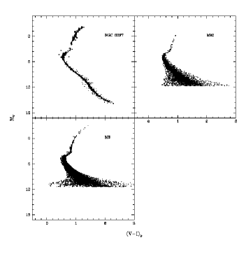
Figure 1: CMDs of NGC 6397, M92 and M3, after the procedure of removing stars and considering the adopted parameters given in r2000

We selected the models computed by b1994 and g1996 (Padova isochrones), tracks developed by d1996 (Yale isochrones) and models by c1998  c1999 (Pisa isochrones). We chose them as they were published in the theoretical plane (HRD). Every model is computed for different input data (metallicities, ages, opacities, stellar atmospheres, etc.), resulting in differences between the isochrones. On the other hand, every model uses different forms of conversion between the theoretical and the observational plane. Because this lack of uniformity may influence the estimation of the age, we limited this additional uncertainty by using the same transformation to each set of isochrones: tabulations of bolometric corrections and colours determinated from the SED extracted from the spectral library of Kurucz b2000 .

3 The method and the age of NGC 6397, M92 and M3

Let S and M be the number of observed stars and synthetic stars generated from a particular stellar model in CMDs of a GC. If both CMDs are binned in a grid of B bins, the probability of having gathered the data under a particular model is the likelihood function, which is given in 1. By $m_{i}$ we denote the number of synthetic stars placed on the $i^{th}$ bin and by $s_{i}$ the number of observed stars inside of the $i^{th}$ bin.

Since there is not a unique configuration of a synthetic CMD of a GC, we generate 1000 different synthetic configurations of the CMD originating from every isochrone of age $t_{i}$. Subsequently we draw the observational CMD and the synthetic CMDs within a grid of B cells. We then count the number of stars $m_{i}$ in each cell for every CMD. In the next step we first calculate log W between two synthetic CMDs (generated from the same isochrone of age $t_{i}$). Secondly, we estimate log W for a new couple of different synthetic samples and continue determining the value of log W between different samples until 500 couples are completed (model–model comparison). The values computed of log W give a distribution of log W, which is represented as the non–shaded region in the histogram (Fig. 2).

We calculate the model–model distribution to compare it with the distribution of frequencies of log W determinated from comparing observational and synthetic samples (data–model comparison). The data–model distributions are constructed by computing log W for couples between 500 synthetic samples (from the same isochrone of age $t_{i}$) and the observational data. In this way 500 values of log W are computed. The distribution of log W is shown as the shaded area in the histogram of Fig. 2.

Figure 2: Example of the distribution of values of log W for different ages of the Padova isochrones for a sample of 1187 stars in NGC 6397 (see text for details)

We estimate the interval of confidence by using the $\chi^{2}$ statistical test, as suggested by p1986 , between the observational and synthetic data and for every evolutionary model. We chose the lowest value of $\chi^{2}$, $\chi^{2}_{min}$. The quantity increases when we move away from the best fit. The values of the confidence levels for a parameter and its respective probabilities (in percent) for data distributed in form of a Gaussian curve were taken from the statistical tables of p1986 . The estimate of the age is given by the age of the isochrone that corresponds to the minimal distance obtained between the Gaussian median fits to the model–model and data–model distributions (14.75 Gyr in Fig. 2). The full details of the approach are presented in r2000 .

$$\mbox{prob}(\mbox{data}\mid\mbox{model})=\frac{S!(M+B-1)!}{(M+S+B-1)!}\cdot W$$ (1)

where W is given by

$$W=\prod^{B}_{i=1}\frac{(m_{i}+s_{i})!}{m_{i}!s_{i}!}=\prod^{B}_{i=1}\,{m_{i}+s_{i}\choose s_{i}}\$$ (2)

Table 1: Summary of the results of the best estimate of the age of the samples considered in this work, for every evolutionary model

Evolutionary	Z of the	$\chi^{2}_{min}$	$\chi^{2}_{red}$	Best estimate	Interval of 99%
Model	Isochrone			of t [Gyr]	of confidence
NGC 6397	1187 stars	B=14400
Padua	0.0004	1352.81	2.82	14.50	[14.3 - 15.1]
Yale	0.0004	1089.04	2.34	14.00	[13.8 - 14.3]
NGC 6397	373 stars	B=8400
Padua	0.0004	232.84	1.41	14.25	[13.7 - 15.6]
Yale	0.0004	206.80	1.25	14.00	[13.3 - 15.1]
Pisa	0.0002	249,95	1.41	13.00	[11.9 - 14.2]
M92	4846 stars	B=12000
Padua	0.0001	2221.63	1.31	14.75	[14.5 - 15.4]
Yale	0.0002	2455.26	1.42	15.00	[14.6 - 15.7]
M92	1482 stars	B=12000
Padua	0.0001	678.79	1.73	15.00	[14.8 - 15.5]
Yale	0.0002	769.67	1.91	15.00	[14.7 - 15.5]
Pisa	0.0002	832.86	2.06	12.00	[11.8 - 12.1]
M3	10333 stars	B=14400
Padua	0.0004	3558.38	1.59	15.75	[15.7 - 15.9]
Yale	0.0004	3037.01	1.37	16.00	[15.9 - 16.3]
M3	4929 stars	B=14400
Padua	0.0004	1038.53	2.14	16.25	[16.2 - 16.6]
Yale	0.0004	757.20	1.68	16.00	[15.9 - 16.3]
Pisa	0.0002	1120.65	2.45	14.00	[13.9 - 14.2]

References

- (1) G. Bertelli et al.: A&AS 106, 275 (1994)
- (2) G. Bruzual: private communication (2000)
- (3) S. Cassisi et al.: A&AS 129, 267 (1998)
- (4) S. Cassisi et al.: A&AS 134, 103 (1999)
- (5) F. D’Antona: private communication (1999)
- (6) P. Demarque et al.: http://www.astro.yale.edu/demarque/astronomy.html (1996)
- (7) L. Girardi et al.: A&AS 117, 113 (1996)
- (8) I. King: private communication (1999)
- (9) W. Press et al.: Numerical Recipes in Fortran. (CU press 1986)
- (10) M. Rengel: Estimation de la edad de Cúmulos Globulares a partir de Diagramas Color–Magnitud. MSc Thesis, Univ. de Los Andes, Mérida–Venezuela (2000)
- (11) M. Rengel et al.: ‘The determination of the age of Globular Clusters: a statistical approach’. In: Extragalactic Star Clusters, IAU Symposium conference at Pucón, Chile, March 12–16, 2001, ed. by E. Grebel, D. Geisler, and D. Minniti (IAU Symposium Series, 2002).
- (12) A. Rosenberg: private communication (1999)
- (13) P. Saha: AJ 115, 1206 (1998)