Acceleration and Parallax Effects in Gravitational Microlensing

Abstract

To generate the standard microlensing light curve one assumes that the relative motion of the source, the lens, and the observer is linear. In reality, the relative motion is likely to be more complicated due to accelerations of the observer, the lens and the source. The simplest approximation beyond the linear-motion assumption is to add a constant acceleration. Microlensing light curves due to accelerations can be symmetric or asymmetric depending on the angle between the acceleration and the velocity. We show that it is possible that some of the previously reported shorter marginal parallax events can be reproduced with constant-acceleration models, while the longer, multi-year parallax events are ill-fitted by such models. We find that there is a generic degeneracy inherent in constant-acceleration microlensing models. We also find that there is an equivalent degeneracy in parallax models, which manifests itself in short-duration events. The importance of this new parallax degeneracy is illustrated with an example, using one of these marginal parallax events. Our new analysis suggests that another of these previously suspected parallax candidate events may be exhibiting some weak binary-source signatures. If this turns out to be true, spectroscopic observations of the source could determine some parameters in the model and may also constrain or even determine the lens mass. We also point out that symmetric light curves with constant accelerations can mimic blended light curves, producing misleading Einstein-radius crossing time-scales when fitted by the standard ‘blended’ microlensing model; this may have some effect on the estimation of optical depth.

1 Introduction

A decade ago Gould (1992) suggested that the Earth’s orbital motion may affect long duration events of gravitational microlensing, producing a periodic modulation of the event light curve. The first such example of this behaviour was detected by Alcock et al. (1995), and a number of additional events have been reported by several groups (e.g., Mao 1999; Smith, Mao & Woźniak 2002a; Bennett et al. 2002a; Bond et al. 2001). However, most of these events were of relatively short duration and showed a strong asymmetry in the light curves, rather than a yearly modulation. Two events were long enough to make a yearly modulation clearly noticeable: OGLE-1999-BUL-32 = MACHO-99-BLG-22 (Mao et al. 2002; Bennett et al. 2002b) and OGLE-1999-BUL-19 (Smith et al. 2002b).

While the Earth’s motion may generate a photometric parallax effect, a similar anomaly may be due to binary motion of the source (sometimes referred to as ‘xallarap’; Griest & Hu 1992; Han & Gould 1997; Paczyński 1997) and/or the lens. In fact such a binary-source modulation was detected in the microlensing event MACHO-SMC-1 (Alcock et al. 1997; Palanque-Delabrouille et al. 1998; Udalski et al. 1997) and MACHO 96-LMC-2 (Alcock et al. 2001). While in these two cases the binary source period was much shorter than the event time scale, an alternative situation may also be encountered. In fact, Smith et al. (2002b) pointed out that even in the case of a very long event exhibiting an annual modulation of its light curve, a model based on a binary source moving with a one year orbital period and suitable inclination and orientation of the orbit may generate a light curve identical to that expected from the parallax effect. While such a coincidence is very unlikely, it is also verifiable in that a binary source should display periodic variations in its radial velocities.

As most parallax microlensing events are not very long it is likely that the effects they show may be well described with a constant acceleration of the Earth, the lens and/or the source, with no need to invoke a specific orbit. The aim of this paper is to investigate this possibility and to present several consequences of the proposed approach. In Section 2 we describe a simple model that incorporates a constant-acceleration term into the microlensing formalism. We then test the efficacy of this model in Section 3 by fitting a number of microlensing events that have been previously identified as exhibiting variations from the standard constant-velocity model of microlensing. The events that we have selected were all identified as potential parallax microlensing events, and in this section we aim to test whether this constant-acceleration model is able to successfully reproduce this behaviour. In this section we also mention that there is a generic degeneracy with the constant-acceleration model, and that there may be an equivalent degeneracy for parallax models. In Section 4 we summarise our work and discuss some of the implications of our findings. In particular, we note that the effect of constant-acceleration perturbations is likely to be of little importance for binary lenses, and such perturbations are therefore most-likely to be due to accelerations of the observer and/or the source.

2 A simple Model

In the simplest case of a microlensing event, the light curve is calculated assuming that the relative motion of the source, the lens, and the observer is linear and constant (Paczyński 1986). The next step in allowing for a more complicated relative motion is to expand it in a power series, and to retain the first two terms, i.e. the velocity, ${\bf v}$, and the acceleration, ${\bf a}$. For the purposes of this paper, we define the velocity, ${\bf v}$, to be the velocity of the lens relative to the observer-source line-of-sight. This acceleration is therefore a relative acceleration, but since the following analysis is likely to be valid only for lenses in inertial motion (see Section 4), this acceleration can be thought of as the acceleration of the observer and/or the source. An acceleration related velocity vector may be defined as ${\bf v_{a}}={\bf a}t_{\rm E}$, where $t_{\rm E}$ is the event time scale: $t_{\rm E}=r_{\rm E}/v$, $r_{\rm E}$ is the Einstein radius and $v$ is the velocity at the minimum separation (peak magnification). We expect that any ‘anomaly’ in the light curve will depend on two dimensionless numbers: the ratio of the two velocities: ${\cal A}=v_{a}/v$, and the angle between them $\theta$. Notice ${\cal A}$ is simply the physical acceleration in units of $r_{\rm E}/t_{\rm E}^{2}$.

In general, an acceleration will produce asymmetry in the microlensing light curve, and this is the effect which is used to select parallax events. However, if the acceleration is mostly in the direction perpendicular to the velocity vector ${\bf v}$ then there will be no asymmetry, just a change in the shape that may be difficult to notice.

Fig. 1 shows four example light curves with different accelerations. All four cases have a minimum impact parameter of $u_{0}=0.1$, and the source is assumed to move along the $x$-axis in the absence of acceleration. The dimensionless acceleration parameters along the $x$ and $y$ directions, ${\cal A}_{x}$ and ${\cal A}_{y}$, are indicated in each panel. The top left panel shows a light curve in which the acceleration is $45^{\circ}$ from the $x$-axis while the bottom left panel shows an example where the acceleration is in the same direction as the source motion. As expected, both light curves show clear asymmetries. The two right panels show light curves in which the acceleration is perpendicular to the $x$-axis. The light curves are symmetric in such cases. The effect of acceleration may not be noticed, and a standard fit forced upon the event may generate incorrect values of the impact parameter and the event time scale; we return to this issue briefly in the discussion. A thorough analysis of all such possibilities in current experiments is beyond the scope of this paper. Instead, we concentrate on the readily available candidate parallax events, in order to check how many of them can be well fitted by adding an acceleration vector to the standard model.

3 Analysis of Candidate Parallax Microlensing Events Using A Constant Acceleration Model

In this section we implement the above constant-acceleration microlensing model and test its efficacy by fitting a number of microlensing events. By analysing previously identified candidate parallax microlensing events, we aim to investigate whether this constant-acceleration model is able to suitably reproduce the observed (i.e. seemingly parallactic) behaviour.

3.1 Constant Acceleration Model

We shall first outline the standard constant-velocity microlensing model. For the standard microlensing light curve, the source position (in units of Einstein radius) is given by

$$x={t-t_{0}\over t_{\rm E}}\equiv x_{0}(t),~{}~{}~{}y=u_{0},$$ (1)

where $t_{0}$ is the time of maximum magnification and $u_{0}$ is the corresponding (minimum) impact parameter. The magnification is given by (Paczyński 1986)

$$A(t)={u^{2}+2\over u\sqrt{u^{2}+4}},~{}~{}~{}u=\sqrt{x^{2}+y^{2}}.$$ (2)

With acceleration, the $(x,y)$ coordinates must be modified to

$$x=x_{0}(t)+{1\over 2}~{}{\cal A}\cos\theta~{}x^{2}_{0}(t),~{}~{}~{}y=u_{0}+{1\over 2}~{}{\cal A}\sin\theta~{}x^{2}_{0}(t),$$ (3)

where $x_{0}(t)$ is defined in eq. (1), ${\cal A}$ is the physical acceleration in units of $r_{\rm E}/t_{\rm E}^{2}$, and the magnification is again calculated using eq. (2). Notice that, since the transverse velocity changes, $t_{\rm E}$ should be understood as the Einstein radius crossing time corresponding to the transverse velocity $v$ at time $t_{0}$. Also, in general, $u_{0}$ may no longer rigorously be the minimum impact parameter, but may still provide a useful approximation, particularly if ${\cal A}$ is small.

To fit a microlensing light curve with the standard model, one needs a minimum of four parameters, $u_{0}$, $t_{0}$, $t_{\rm E}$, and the baseline flux (or magnitude), $f_{0}$. One also often requires an extra blending parameter, which accounts for the additional light contributed by the lens and/or other stars in the crowded field. To do this, we use a parameter, $f_{\rm s}$, defined as the fraction of light contributed by the lensed source at the baseline. To incorporate the constant acceleration, we need two extra parameters, ${\cal A}$ and the angle $\theta$ (or equivalently, ${\cal A}_{x}$ and ${\cal A}_{y}$).

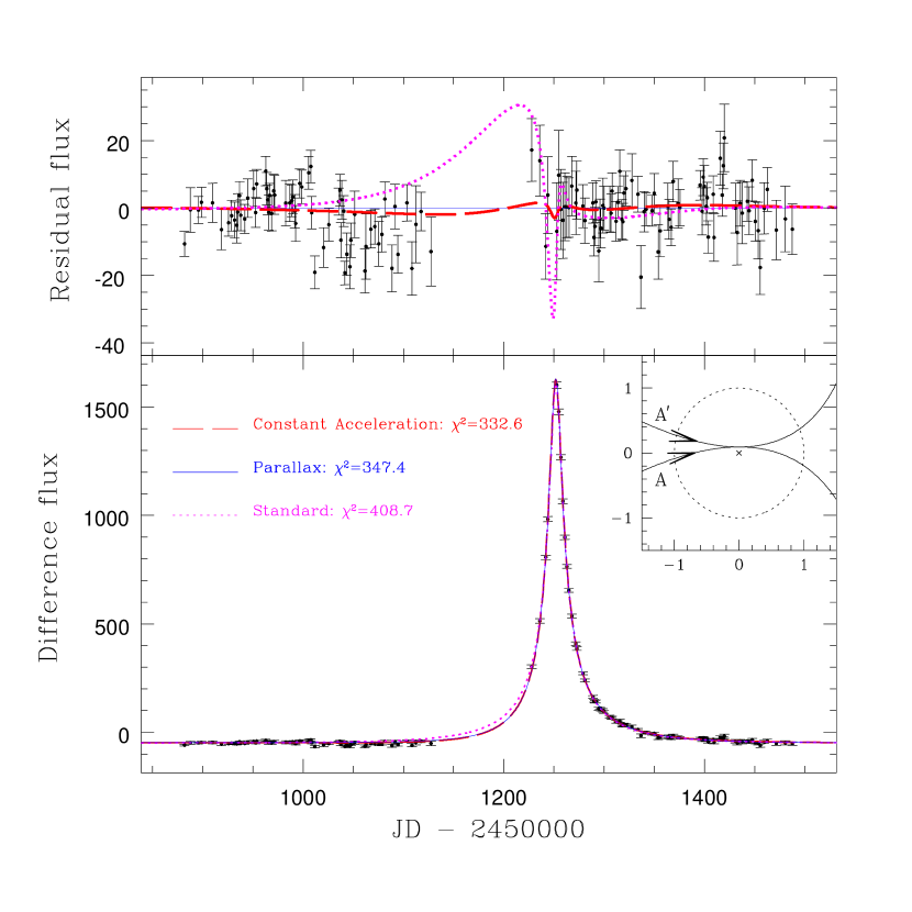
Figure 2: The I-band light curve for OGLE-II event sc6_2563 from difference image analysis, with flux given in units of 10 ADU. The data for the first season has been omitted from this plot. The $I$-band baseline magnitude for this event is 17.7, rising to 15.1 at the peak. The top panel shows the residual flux (the observed data points with the parallax model subtracted). This figure shows that the constant-acceleration model and the parallax model produce very similar fits, with the former model providing a slight improvement in $\chi^{2}$. However, both models appear to over-predict the flux around $1000<t<1150$ days. The inset illustrates the two possible trajectories for the constant-acceleration model, described by the two fits A (bottom) and $\rm{A}^{\prime}$ (top) given in Table 1. The dotted circle represents the size of the event’s Einstein radius, $r_{\rm E}$, and the axes are in units of this Einstein radius. Both trajectories result in identical light curves, even though the parameter values for $t_{\rm E}$, ${\cal A}$ and $\theta$ differ (see Section 3 and Appendix A1 for a discussion of this degeneracy).

We look for any degeneracy in the parameter space for this constant-acceleration model by fitting each event 1000 times, with the initial parameter guesses selected from wide range of randomly chosen values. We find that two sets of parameters exist for each $\chi^{2}$ minimum. The parameters are identical except for the time-scale, $t_{\rm E}$, and the acceleration parameters, ${\bf{\cal A}}$ and $\theta$. However, the magnitude of the physical acceleration in units of $r_{\rm E}/{\rm day}^{2}$ (i.e., $\left|{\bf a}/r_{\rm E}\right|={\bf{\cal A}}/t_{\rm E}^{2}$, as defined in §2) is the same for both fits, although the direction of this vector (i.e., $\theta$) differs. In Appendix A1, we show that this degeneracy can be understood analytically. An example of this degeneracy is illustrated in the inset of Fig. 2 for the microlensing event sc6_2563; even though the two trajectories look very different they both result in identical light curves. The full analysis of the event sc6_2563 is described in Section 3.2.1.

It should be noted that one may expect this degeneracy to manifest itself in parallax models. In particular, this could be important for short-duration events that exhibit weak parallax signatures, since in this case the Earth’s acceleration can be approximated to be constant (i.e. the regime in which this degeneracy is expected to occur). By testing this hypothesis on the event sc6_2563, we are able to verify the existence of this degeneracy. However, it seems that this may only become apparent for weak parallax candidates, since a more convincing parallax candidate (sc33_4505; Section 3.2.3) shows no such degeneracy (see Appendix A). A full discussion of this degeneracy, including the application to events sc6_2563 and sc33_4505, can be found in Appendix A2.

3.2 Analysis of candidate parallax microlensing events

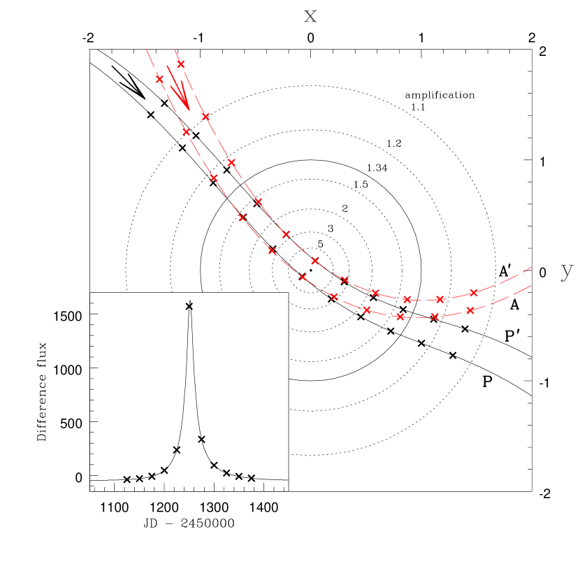
Figure 5: The degenerate parallax (solid lines) and constant-acceleration (dashed lines) trajectories for the OGLE-II event sc6_2563. These trajectories are described in the lens plane and correspond to the paths taken by the lens relative to the observer-source line-of-sight (i.e. the origin). Each degenerate fit is labelled according to Table 1. Note that the $A^{\prime}$ trajectory has been rotated so that its acceleration is pointing in the same direction as the $A$ trajectory (the rotation does not affect the light curve). The contours of constant amplification are represented by the dotted circles (since the amplification is dependent on the separation of the lens from the observer-source line-of-sight; see eq. 2), and the Einstein radius is given by the solid circle. The inset shows the light curve for this event. The crosses on each trajectory denote 25 day intervals, as labelled on the inset light curve. Note that all of the trajectories presented here result in (practically) the same light curve.

We proceed by analysing a selection of events that have previously been identified as candidate parallax microlensing events. The parallax model used here requires 7 parameters: the 5 parameters from the standard model plus two additional parameters to describe the lens trajectory in the ecliptic plane, namely the Einstein radius projected onto the observer plane, $\tilde{r}_{\rm E}$, and an angle $\psi$ in the ecliptic plane. $\psi$ is defined as the angle between the heliocentric ecliptic $x$-axis and the normal to the trajectory (This geometry is illustrated in Fig. 5 of Soszyński et al. 2001). These candidate parallax events have been selected to provide a broad range of parallactic signatures, ranging from marginal cases to those displaying more prominent effects.

3.2.1 sc6_2563

Table 1: The best standard model (first row), the best parallax models (second and third rows), and the best constant-acceleration model (fourth and fifth rows) for the OGLE-II event sc6_2563. The final column shows the $\chi^{2}$ and the number of degrees of freedom (dof) for each model. The parameters are explained in §2 & §3. $\theta$ is given in units of radians. There are two sets of constant-acceleration parameters since each $\chi^{2}$ minimum has two degenerate fits with differing values for $t_{\rm E}$, ${\cal A}$ and $\theta$. There are also two sets of parallax parameters, owing to the parallax degeneracy that is analogous to this constant-acceleration degeneracy. Both degeneracies are discussed in Section 3.1 and Appendix A.

Model	$t_{0}$	$t_{\rm E}$ (day)	$u_{0}$	$f_{0}$	$f_{\rm s}$	$\psi$	$\tilde{r}_{\rm E}$ (au)	${\cal A}$	$\theta$	$\chi^{2}$/dof
S	$1251.971\pm 0.054$	$89.2\pm 2.2$	$0.0758^{+0.0026}_{-0.0025}$	$169.43\pm 0.41$	$0.802^{+0.026}_{-0.025}$	—	—	—	—	408.7/216
P	$1257.4^{+4.1}_{-1.1}$	$71.5^{+1.8}_{-1.3}$	$0.1289\pm 0.0057$	$169.98^{+0.41}_{-0.42}$	$1.000^{+0}_{-0.022}$	$0.134^{+0.089}_{-0.026}$	$4.021\pm 0.086$	—	—	347.4/214
$\rm{P}^{\prime}$	$1247.6^{+1.1}_{-3.7}$	$73.4^{+1.2}_{-0.7}$	$0.368^{+0.074}_{-0.057}$	$169.91\pm 0.41$	$1.000^{+0}_{-0.020}$	$0.129^{+0.091}_{-0.025}$	$3.8^{+1.9}_{-0.9}$	—	—	348.2/214
A	$1251.774\pm 0.057$	$71.78^{+2.39}_{-0.52}$	$0.09253^{+0.00063}_{-0.00353}$	$170.32\pm 0.41$	$1.000^{+0}_{-0.040}$	—	—	$0.496^{+0.065}_{-0.069}$	$4.233^{+0.053}_{-0.050}$	332.6/214
$\rm{A}^{\prime}$	$1251.774\pm 0.057$	$74.88^{+2.55}_{-0.45}$	$0.09253^{+0.00063}_{-0.00353}$	$170.32\pm 0.41$	$1.000^{+0}_{-0.041}$	—	—	$0.539^{+0.082}_{-0.079}$	$2.072^{+0.049}_{-0.055}$	332.6/214

This event was detected by the OGLE collaboration (Udalski et al. 2000). Its asymmetric nature was identified during a parallax search of the OGLE-II database (Woźniak et al. 2001), reported in Smith et al. (2002a). It was classified as a ‘marginal’ candidate, since the deviations from the standard model are not particularly pronounced and the improvement in $\chi^{2}$ is only slight. The best-fit parameters for the standard and parallax models are given in Table 1, and the corresponding light curves are plotted in Fig. 2. The inset of this figure shows the two degenerate trajectories for the constant-acceleration model; as was discussed above, each $\chi^{2}$ minimum has two degenerate fits. Both of these trajectories produce identical light curves, even though the parameter values for $t_{\rm E}$, ${\cal A}$ and $\theta$ differ. This table also includes an additional parallax fit, which has a $\chi^{2}$ difference of 0.8 compared to the best-fit parallax model. This is a manifestation of the parallax degeneracy that is analogous to this constant-acceleration degeneracy. See Section 3.1 and Appendix A for a discussion of these degeneracies.

It would be expected that a constant-acceleration fit may be suitable for this event since the duration is not very long, and the asymmetry shows no signs of modulation. Indeed, when this event is fit with the above constant-acceleration model the best-fit $\chi^{2}$ value improves upon the best-fit parallax value from 347.4 to 332.6. If the error bars are rescaled so that the best-fit $\chi^{2}$ per degree of freedom is renormalised to unity, then the difference in $\chi^{2}$ between these two fits is 9.5 for no additional free parameters, i.e. a significant 3-$\sigma$ improvement. The best-fit parameters and corresponding light curve for the acceleration model are given in Table 1 and Fig. 2, respectively. From this figure it is clear that the parallax and constant-acceleration models produce similar fits. However, both models seem to over-predict the flux around $1000<t<1150$ days, implying that there may be some non-constant contribution to the acceleration that is not parallactic in nature. Notice that the standard microlensing model predicts a blending parameter $f_{\rm s}\approx 0.8$ while other models predict $f_{\rm s}\approx 1$. Correspondingly, the Einstein radius crossing time is about 25% larger for the standard model than for the other models; this has implications for the optical depth estimate in the experiments (see Section 4).

3.2.2 OGLE-1999-CAR-1

This event was detected in real-time by the OGLE Early Warning System (Udalski et al. 1994) toward the Carina spiral arm. It has been found to exhibit systematic deviations from the standard model (Mao 1999). The duration for this event is well over 100 days, and it was concluded that these deviations are due to the parallax effect.

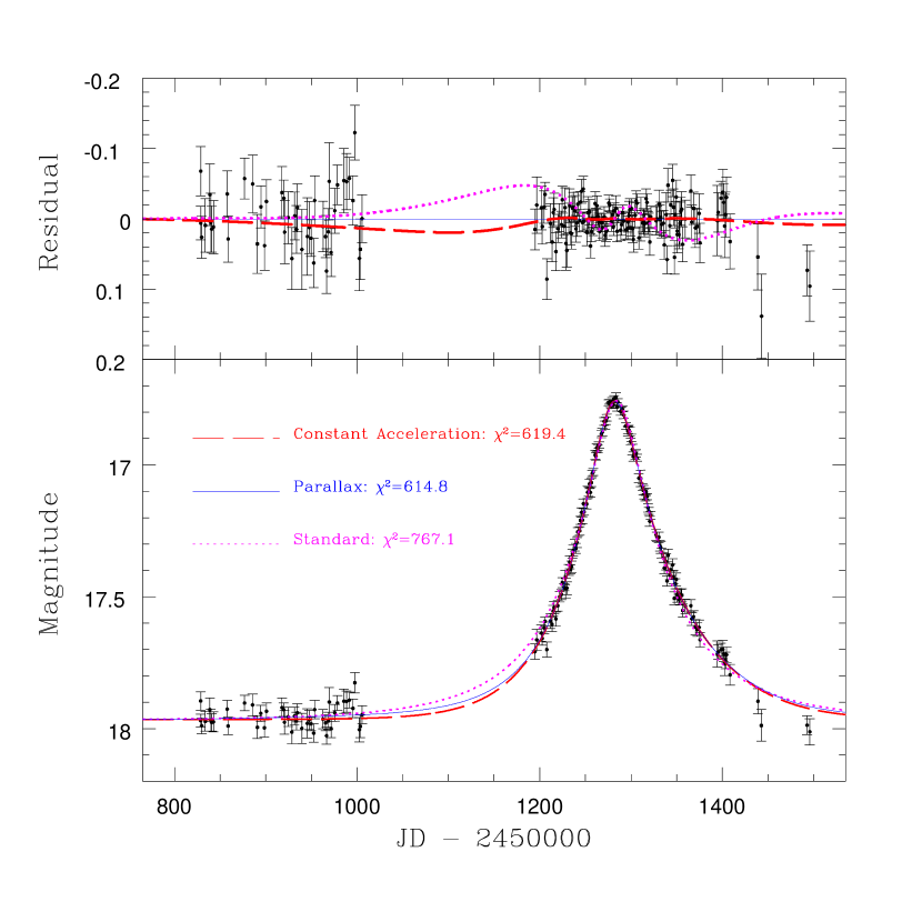
Figure 3: The I-band light curve for event OGLE-1999-CAR-1 from difference image analysis. The data for the first season have been omitted from this plot. The top panel shows the residual magnitude (the observed data points with the parallax model subtracted). This shows that the parallax model and the constant-acceleration model produce almost identical fits.

As with sc6_2563, the deviations from the standard model for OGLE-1999-CAR-1 show no signs of modulation, and so one would expect that this event may be suitably approximated by a constant acceleration model. This appears to be correct, since the best-fit constant-acceleration model is able to prove a very similar fit (with a slightly worse $\chi^{2}$ value of 619.4 compared with the parallax best-fit value of 614.8). The best-fit parameters for all models are given in Table 2, and the corresponding light curves are shown in Fig. 3. It is interesting to note that both of the degenerate acceleration fits have values of ${\cal A}=v_{a}/v$ greater than 1 (${\cal A}=1.4$, and ${\cal A}=2.4$). This implies that $v_{a}$, the change in velocity due to this constant acceleration in a time $t_{\rm E}$, is greater than the $v$, the velocity at the point of closest approach.

Also of note is the difference in $t_{\rm E}$ among the three models. The values range from $t_{\rm E}=126$ days for the parallax model, to as much as $t_{\rm E}=190$ days for the constant-acceleration model. These differences in the time-scale are closely connected with their differences of the blending parameter, due to potential degeneracy between these two parameters (Woźniak & Paczyński 1997).

Table 2: The best standard model (first row), the best parallax model (second row), and the best constant-acceleration model (third and fourth rows) for OGLE-1999-CAR-1. The parameters are explained in §2 & §3. $\theta$ is given in units of radians. There are two sets of constant-acceleration parameters since each $\chi^{2}$ minimum has two degenerate fits with differing values for $t_{\rm E}$, ${\cal A}$ and $\theta$ (see Section 3.1 and Appendix A1).

Model	$t_{0}$	$t_{\rm E}$ (day)	$u_{0}$	$f_{0}$	$f_{\rm s}$	$\psi$	$\tilde{r}_{\rm E}$ (au)	${\cal A}$	$\theta$	$\chi^{2}$/dof
S	$1284.05\pm 0.13$	$130.7^{+6.9}_{-6.4}$	$0.207^{+0.014}_{-0.013}$	$17.9681\pm 0.0021$	$0.525^{+0.043}_{-0.040}$	—	—	—	—	767.1/722
P	$1285.4^{+1.3}_{-1.7}$	$126^{+15}_{-10}$	$0.281^{+0.019}_{-0.018}$	$17.9677\pm 0.0021$	$0.48^{+0.12}_{-0.11}$	$1.22^{+0.33}_{-0.21}$	$7.8^{+1.7}_{-1.3}$	—	—	614.8/720
A	$1282.46\pm 0.20$	$144^{+29}_{-17}$	$0.162^{+0.030}_{-0.033}$	$17.9654\pm 0.0020$	$0.391^{+0.087}_{-0.091}$	—	—	$1.37^{+0.37}_{-0.61}$	$4.449^{+0.035}_{-0.044}$	619.4/720
$\rm{A}^{\prime}$	$1282.46\pm 0.20$	$190^{+52}_{-31}$	$0.162^{+0.030}_{-0.033}$	$17.9654\pm 0.0020$	$0.391^{+0.087}_{-0.091}$	—	—	$2.38^{+1.50}_{-0.81}$	$1.922^{+0.041}_{-0.033}$	619.4/720

3.2.3 sc33_4505

This OGLE-II event was also found during the search of Smith et al. (2002a), but was classified as a ‘convincing’ parallax candidate. Unlike sc6_2563, the duration of this event was much longer ($t_{\rm E}\sim 200$ days, cf. $t_{\rm E}\sim 100$ days for sc6_2563), and the data show clear signs of deviation from the standard model in both the rising and declining branch of the light curve. Therefore, if this asymmetry is indeed due to the parallax effect then one would suspect that a constant-acceleration model would be unable to reproduce this behaviour (since the acceleration of the Earth cannot be considered constant during this time span). On the other hand, if this asymmetry is due to other causes, the constant-acceleration model may provide a better fit.

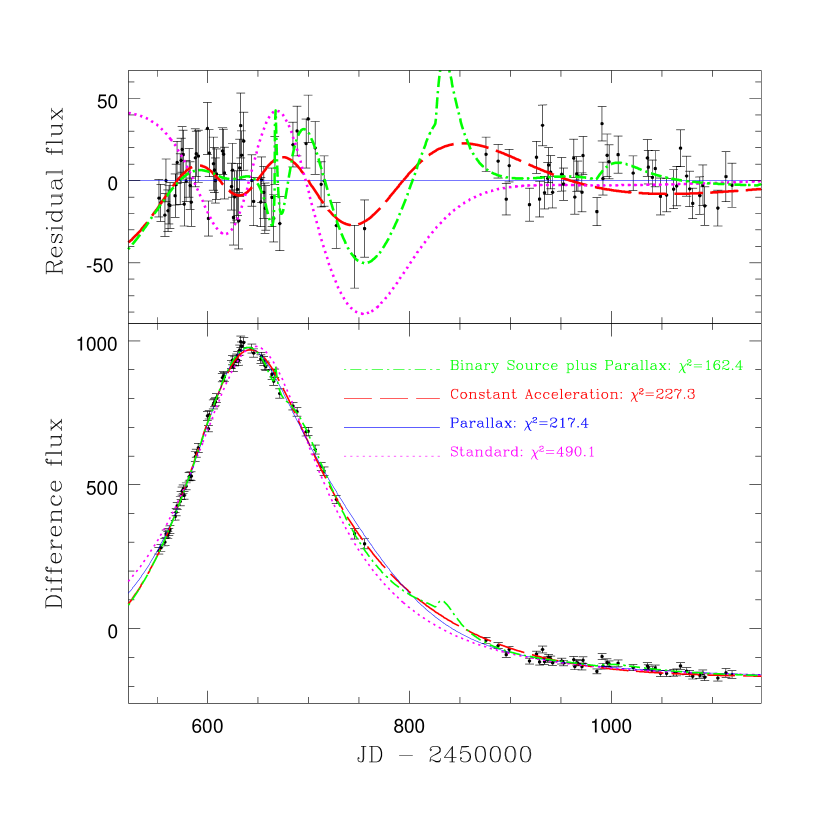
Figure 4: The I-band light curve for the OGLE-II event sc33_4505 from difference image analysis. The data for the third season have been omitted from this plot. The $I$-band magnitude for this event is 15.7 at the baseline and rises to 15.0 at the peak. The top panel shows the residual flux (the observed data points with the parallax model subtracted). It is clear from this panel that there are systematic residuals from the parallax fit. The constant acceleration model appears to fit the data much better, but this still seems to be deficient. However, the ‘binary-source plus parallax’ model provides the best-fit (see Section 3.2.3). Spectroscopic observations could confirm whether this event is being affected by binary motion of the source; such observations would enable constraints to be put on some of the model parameters, and may also result in a direct measurement of the lens mass.

The best-fit parameters for the standard and parallax models are given in Table 3, and the corresponding light curves are shown in Fig. 4. A problem arises when this event is fit with the constant-acceleration model, in that two minima are identified, with $\chi^{2}=187.3$ and $\chi^{2}=227.3$, respectively. Due to the degeneracy discussed in §3 and Appendix A1, there are two degenerate fits corresponding to each of these two $\chi^{2}$ values. The two degenerate fits that correspond to $\chi^{2}=187.3$ have extremely large time-scales ($t_{\rm E}=1812.8\,{\rm day}$ and $t_{\rm E}=4880.5\,{\rm day}$), and the lensed star contributes only 2.3 per cent of the total baseline light (i.e., $f_{\rm s}=0.023$). These values do not seem physical to us, and therefore the fits corresponding to this $\chi^{2}$ minimum are disregarded. The best-fit parameters for the two degenerate fits corresponding to $\chi^{2}=227.3$ are more ‘feasible’; they are given in Table 3 and the corresponding light curve is shown in Fig. 4.

However, the discarded ‘unfeasible’ constant-acceleration models have an overall best $\chi^{2}$ value (187.3). Since this $\chi^{2}$ value is better than the best-fit parallax model, it highlights that there could be a deficiency in the parallax fit. This deficiency in the parallax fit can be seen in the residual plot in Fig. 4; systematic residuals from the parallax model can clearly be seen, and the remaining ‘feasible’ constant-acceleration fit is also unable to successfully reproduce this behaviour.

These residuals from the parallax model could imply that this event is exhibiting some weak binary-source signatures (see, for example, Alcock et al. 2001). We performed a preliminary investigation to test this hypothesis, fitting the event with a simple binary-source model. The basic details of this model can be found in Smith et al. (2002b), but the version used here has two differences from the earlier work: firstly, it incorporates the parallax motion of the Earth (which, in most cases, should have an effect on the light curve since the duration of this event is well over one year); and secondly, only face-on elliptical orbits are considered.

The best binary-source plus parallax fit that we are able to identify has a much better $\chi^{2}$ value ($\chi^{2}=162.4$) compared to all of the previous models. However, we find a range of possible binary-source fits with $\chi^{2}$ less than 180. The single best-fit solution is presented in Table 4 and Fig. 4. This model predicts a very large value for the Einstein radius projected into the observer plane ($\tilde{r}_{\rm E}=108$ au), which implies that the parallax motion of the Earth has little effect on the light curve, i.e., the majority of the perturbations from the standard model arise due to the binary nature of the source. It seems that this model is able to fit the systematic residuals from the parallax model, although it predicts peculiar bumps in the light curve (most notably during the break between observing seasons). We present this model to show that such fits are possible, but we do not attempt a more detailed analysis of this event in this work.

If this event is indeed affected by the binary motion of the source then a spectroscopic followup should find the source to be a spectroscopic binary, and this would reduce the number of free parameters in our model. Furthermore, if the projected separation of the two sources can be estimated, then this would enable us to make a direct determination of the lens mass (Han & Gould 1997). The source baseline magnitude (including blending) is about $I=15.7$ mag, and so it should be within easy reach of modern large telescopes.

Table 3: The best standard model (first row), the best parallax model (second row), and the best constant-acceleration model (third and fourth rows) for the OGLE-II event sc33_4505. The parameters are explained in §2 & §3. $\theta$ is given in units of radians. There are two sets of constant-acceleration parameters since each $\chi^{2}$ minimum has two degenerate fits with differing values for $t_{\rm E}$, ${\cal A}$ and $\theta$ (see Section 3.1 and Appendix A1).

Model	$t_{0}$	$t_{\rm E}$ (day)	$u_{0}$	$f_{0}$	$f_{\rm s}$	$\psi$	$\tilde{r}_{\rm E}$ (au)	${\cal A}$	$\theta$	$\chi^{2}$/dof
S	$647.22\pm 0.32$	$165.9^{+8.6}_{-8.4}$	$0.412^{+0.031}_{-0.028}$	$1146.3\pm 1.5$	$0.637^{+0.069}_{-0.058}$	—	—	—	—	490.1/179
P	$654.8^{+3.6}_{-3.5}$	$191^{+30}_{-21}$	$-0.213^{+0.054}_{-0.055}$	$1144.4^{+1.7}_{-2.1}$	$0.40\pm 0.11$	$3.1372^{+0.0086}_{-0.0104}$	$6.33^{+0.52}_{-0.40}$	—	—	217.4/177
A	$642.36\pm 0.46$	$115.38^{+3.44}_{-0.88}$	$0.5596\pm 0.0014$	$1149.4^{+1.3}_{-1.4}$	$1.000^{+0}_{-0.064}$	—	—	$0.561^{+0.033}_{-0.024}$	$4.252\pm 0.015$	227.3/177
$\rm{A}^{\prime}$	$642.36\pm 0.46$	$166.9^{+6.0}_{-2.6}$	$0.5596\pm 0.0014$	$1149.4^{+1.3}_{-1.4}$	$1.000^{+0}_{-0.064}$	—	—	$1.174^{+0.094}_{-0.093}$	$2.268\pm 0.029$	227.3/177

Table 4: The best-fit parameters for the elliptical binary-source model for the OGLE-II event sc33_4505. The first seven parameters correspond to the usual parallax microlensing parameters (see §3), and the final six describe the binary nature of the source. The mass (flux) ratio, ${\cal M}$ (${\cal F}$), is defined as the mass (flux) of the first binary source divided by the total mass (flux) of the two sources. A detailed description of the binary-source model can be found in Smith et al. (2002b). The errors have been omitted since they were found to be misleading, owing to the complexity of the $\chi^{2}$ surface.

$t_{0}$	$t_{\rm E}$ (day)	$u_{0}$	$f_{0}$	$f_{\rm s}$	$\tilde{r}_{\rm E}$	$\theta$
$675.2$	$140.5$	$0.573$	$1143.2$	$1.00$	$107.9$	$5.623$
orbital period (day)	semi-major axis ($r_{\rm E}$)	${\cal M}$	${\cal F}$	eccentricity	phase	$\chi^{2}/\mbox{dof}$
$159.48$	$1.057$	$0.105$	$0.192$	$0.943$	$1.216$	162.415/71

3.2.4 OGLE-1999-BUL-19 and OGLE-1999-BUL-32/MACHO-99-BUL-22

These two events display unambiguous deviations from the standard model. They were detected by the OGLE Early Warning System (with OGLE-1999-BUL-32 being independently detected by the MACHO collaboration’s Alert System, by which it was named MACHO-99-BUL-22). Both of these events also appear in the difference image analysis catalogue of Woźniak et al. (2001), and are labelled sc40_2895 and sc33_3764, respectively. For the purposes of this paper, we fit these events using the OGLE difference image analysis data from Woźniak et al. (2001).

OGLE-1999-BUL-19 (Smith et al. 2002b) displays prominent multiple peaks that are well fit by a parallax model, while OGLE-1999-BUL-32 (Mao et al. 2002; Bennett et al. 2002b) is the longest duration event ever discovered. Both events are suitably fit by the parallax model, and both show significant improvement in $\chi^{2}$ between the standard and parallax models.

Since the microlensing amplification for both of these events lasts well over two years, we expect that a constant-acceleration model may not be adequate to describe their behaviour. By fitting with the constant-acceleration model we find that this is true; neither of these events are well fit. The best-fit $\chi^{2}$ values for these events are given in Table 5. For OGLE-1999-BUL-19, the $\chi^{2}$ for the constant-acceleration model is 11420, which is far worse than the parallax model of 590.1. Similarly, for OGLE-1999-BUL-32, the $\chi^{2}$ for the constant acceleration model is 464.4 compared with 278.2 for the parallax model.

Table 5: The best $\chi^{2}$ values for the two unusual events OGLE-1999-BUL-19 (Smith et al. 2002b) and OGLE-1999-BUL-32 (Mao et al. 2002; Bennett et al. 2002b).

	OGLE-1999-BUL-19	OGLE-1999-BUL-32
Standard $\chi^{2}$/dof	17910/312	576.3/264
Parallax $\chi^{2}$/dof	590.1/310	278.2/261
Constant Acceleration $\chi^{2}$/dof	11420/310	464.4/261

4 Discussion

In this paper, we have illustrated the effect of acceleration on microlensing light curves. We studied whether the known parallax microlensing events can be equally fitted by a model with a constant acceleration. We found that for the shorter marginal parallax microlensing events, the constant acceleration is indeed sufficient. However, for the longest events (notably, OGLE-1999-BUL-32 and OGLE-1999-BUL-19), the constant acceleration fails to provide a satisfactory model, so their parallax nature seems secure.

It is important to examine whether there is an empirical way of separating ‘parallax events’ from ‘microlensing events with acceleration’. For binary lenses it can be shown that such constant-acceleration perturbations are unlikely to be of importance. This can be understood by considering three regimes of binary lenses separately: close binaries (i.e., those with separation $b\ll r_{\rm E}$), intermediate binaries ($b\sim r_{\rm E}$), and wide binaries ($b\gg r_{\rm E}$). One would expect sufficiently large accelerations for close separation binaries. However, unless the impact parameter is extremely small (i.e. the source passes very close to the centre of mass of the lens), it is unlikely that the resulting light curve will be differentiable from a standard single-lens light curve (Gaudi & Gould 1997). Even in the rare cases where such small impact parameters occur, one would expect the primary deviations to be caused by the binary structure, rather than the acceleration (for example, the binary-lens event MACHO-99-BLG-47, Albrow et al. 2002). For intermediate binaries where the separation is of the order of the Einstein radius, one would also expect the primary deviations to arise from the binary structure, rather than the acceleration. Even in the absence of caustic crossings, the effect of acceleration should be relatively small compared to the distortion of the light curve due to the other mass (For example, typical lens geometries - with the source lying in the bulge at a distance of approximately $8\,{\rm{kpc}}$ and the lens lying half-way in between - predict $r_{\rm E}\sim 4~{}{\rm au}~{}(M_{\rm lens}/M_{\odot})^{1/2}$, where $M_{\rm lens}$ is the total lens mass; therefore, for face-on orbits with separations of approximately $1~{}r_{\rm E}$, a typical orbital period is $P\sim 8~{}{\rm yr}~{}(M_{\rm lens}/M_{\odot})^{1/4}$, which implies that the resulting acceleration should produce only weak perturbations to the light curve compared to the distortion from the companion mass). For the case of wide separation binaries, it is clear that the accelerations should be small compared to the Earth’s acceleration, since binaries with separation much greater than $r_{\rm E}$ are expected to have orbital periods of longer than 8 years. Therefore, we conclude that the effect of constant accelerations in binary lenses is unlikely to be of importance.

In principle, there is a simple test to determine whether an acceleration is due to binary motion of the source or the observer: for the case where the acceleration is induced by the source’s binary motion, the source must show (periodic) changes in radial velocity, which can be verified even after the event is over. In Appendix B, we illustrate the expected radial velocities for the simple case of circular binary orbits. We find that the expected radial velocity amplitude is of the order of $35{\rm\,km\,s^{-1}}{\cal A}^{1/4}\sin i/\cos^{1/4}i$, where $i$ is the inclination angle; there is also some weak dependency on $t_{\rm E}$, the transverse velocity of the lens, $v$, and the masses. The expected orbital period depends on the unknown lens transverse velocity and the inclination angle, but is of the order of $\sim$ years. This radial velocity can, in principle, be measured.

In the right two panels of Fig. 1, we showed that the light curves are symmetric when the acceleration is perpendicular to the source trajectory. In such cases, the effect of acceleration may be difficult to notice. This may even be true for some cases for which the acceleration is not exactly perpendicular to the source motion, particularly since the real light curves have significant gaps due to bad weather, etc. If we force the standard fit to the microlensing light curve, the time-scale obtained from the fit may be different from the true value. To illustrate the effect, we generate artificial light curves using Monte Carlo simulations. We adopt $t_{\rm E}=30$ days, and a sampling frequency of one observation per day; the observations lasts from $-2t_{\rm E}$ to $2t_{\rm E}$ centred around the peak of the light curve. The observational errors are assumed to be 0.05 magnitudes at the baseline and scale according to photon Poisson noise. We find that a standard fit incorporating blending is significantly better than a fit without blending. In other words, a microlensing light curve with constant acceleration can mimic light curves with blending. Interestingly, the fit with blending under-estimates the true $t_{\rm E}$ by 20% for both acceleration values (${\cal A}=\pm 1.5$) shown in the right panels of Fig. 1. This can have important implications for the calculation of optical depth. The optical depth, $\tau$, is estimated from experiments using the following formula (see, for example, Han & Gould 1995),

$$\tau=\frac{\pi}{2N_{*}T_{*}}\sum_{i=1}^{N}\frac{{t_{\rm E}}_{,i}}{\epsilon({t_{\rm E}}_{,i})},$$ (4)

where $N_{*}$ is the total number of monitored stars, $T_{*}$ is the experiment duration in years, $\epsilon({t_{\rm E}}_{,i})$ is the detection efficiency, and ${t_{\rm E}}_{,i}$ is the Einstein radius crossing time for the $i$-th event ($i=1,\ldots,N$). Obviously, if the time-scale is underestimated then this will lead to an underestimation in the optical depth, and vice versa. However, a quantitative analysis requires a detailed knowledge about the binary parameters of the lens and the source, and sampling frequencies in observations. This is clearly an area that deserves further study.

Appendix A Degeneracies

In this appendix we first describe the degeneracy that is found to arise in the constant-acceleration model. This is followed by a discussion of an equivalent degeneracy in the parallax model, which can occur for short duration events where the Earth’s acceleration may be approximated as constant.

A.1 Degeneracy in Constant-Acceleration Models

In Section 3 we discuss the degeneracy inherent in fitting microlensing light curves with the constant-acceleration model. It is found that each $\chi^{2}$ minimum has two corresponding fits, each with differing values of time-scale, $t_{\rm E}$, and the acceleration parameters, ${\cal A}$ and $\theta$. However, the magnitude of the physical acceleration in units of $r_{\rm E}/{\rm day}^{2}$ (i.e., $\left|{\bf a}/r_{\rm E}\right|={\cal A}/t_{\rm E}^{2}$) is the same for both fits, although the direction of this vector (i.e., $\theta$) differs. In this subsection we show analytically why this degeneracy occurs.

Given a combination of parameters (${t_{\rm E}}$, $u_{0}$, etc), the magnitude of the source displacement in the lens plane (in units of the Einstein radius) at a time $(t_{0}+\delta t)$ can be determined from equations (1-3),

$$u^{2}(t_{0}+\delta t)=\left(\hat{a}\cos{\theta}~{}\frac{(\delta t)^{2}}{2}+\frac{\delta t}{{t_{\rm E}}}\right)^{2}+\left(\hat{a}\sin{\theta}~{}\frac{(\delta t)^{2}}{2}+u_{0}\right)^{2},$$ (5)

where $\hat{a}=\left|{\bf a}/r_{\rm E}\right|={\cal A}/t_{\rm E}^{2}$ is the magnitude of the physical acceleration in units of the Einstein radius.

This equation can be expanded to give,

$$u^{2}(t_{0}+\delta t) = \hat{a}^{2}\frac{(\delta t)^{4}}{4}$$ (6)

$$+ \left(\hat{a}\frac{\cos{\theta}}{{t_{\rm E}}}\right)(\delta t)^{3}$$

$$+ \left(\frac{1}{{t_{\rm E}}^{2}}+u_{0}\hat{a}\sin{\theta}\right)(\delta t)^{2}$$

$$+ u_{0}^{2}.$$

For two degenerate solutions $i$ and $j$, the magnitude of the source displacement, $u_{i}(t_{0}+\delta t)$ and $u_{j}(t_{0}+\delta t)$, must be the same for all values of $\delta t$ (since this is required to produce identical light curves), i.e., $u_{i}^{2}(t_{0}+\delta t)=u_{j}^{2}(t_{0}+\delta t)$ for all $\delta t$. Since this is true for all values of $\delta t$, using equation (6) we can equate powers of $\delta t$. This gives the following four equations,

$$\hat{a}_{i} = \hat{a}_{j}$$ (7)

$$\hat{a}_{i}\frac{\cos{\theta}_{i}}{{t_{\rm E}}_{,i}} = \hat{a}_{j}\frac{\cos{\theta}_{j}}{{t_{\rm E}}_{,j}}$$ (8)

$$\frac{1}{{t_{\rm E}}_{,i}^{2}}+u_{0,i}\hat{a}_{i}\sin{\theta}_{i} = \frac{1}{{t_{\rm E}}_{,j}^{2}}+u_{0,j}\hat{a}_{j}\sin{\theta}_{j}$$ (9)

$$u_{0,i}^{2} = u_{0,j}^{2}.$$ (10)

From equations (7) and (10) we can see that both $\hat{a}$ and $u_{0}$ must be constant for degenerate solutions (the sign of $u_{0}$ is irrelevant due to the symmetry of the acceleration model; by taking only $u_{0}>0$ one still obtains the full set of solutions). Also, from equations (8) and (9) we find that the quantities $[\cos\theta/t_{\rm E}]$ and $[1/(t_{\rm E})^{2}+u_{0}\hat{a}\sin\theta]$ must also be constant for degenerate solutions. Therefore, the following two equations must hold for every degenerate solution,

$$\frac{\cos\theta}{t_{\rm E}}=c_{1},$$ (11)

$$\frac{1}{t_{\rm E}^{2}}+u_{0}~{}\hat{a}~{}\sin\theta=c_{2},$$ (12)

where $c_{1}$ and $c_{2}$ are constants defined for any given $\chi^{2}$ minimum. The parameter $\theta$ can then be eliminated from these two equations to give the following expression for $t_{\rm E}$,

$$f(w)=(\hat{a}u_{0}c_{1})^{2}{w}^{3}+(c_{2}^{2}-\hat{a}^{2}u^{2}_{0})w^{2}-2c_{2}w+1=0,$$ (13)

where $w\equiv t_{\rm E}^{2}$. We see that the above equation is a cubic equation in $w$. As the coefficients are all real, the number of real solutions is either one or three. Recall that since $w=t_{\rm E}^{2}$, physical solutions to equation (13) must clearly correspond to positive values of $w$.

As $f(-\infty)=-\infty$, and $f(w=0)=1$, we must have one negative real solution for $w$, which is unphysical and should be discarded. It is easy to show that the number of positive (i.e. physical) solutions for $w$ must be either zero or two. This follows because $f(w=0)=1$ and $f(w=+\infty)=+\infty$. If $f(w)$ is everywhere positive for $w>0$, then the number of positive solutions is obviously zero. If, however, $f(w)$ is negative at some point ${w}_{1}(>0)$, then there must be one positive solution in the region 0 to ${w}_{1}$, and another positive solution in the region ${w}_{1}$ to $+\infty$. This therefore immediately implies that if there is one good constant-acceleration fit (i.e. one physical solution for $w$), then there must be another degenerate fit with the same $\chi^{2}$, just as we have found numerically. These two fits have identical values of $u_{0}$ and $\hat{a}={\cal A}/t_{\rm E}^{2}$, but different values of ${\cal A}$, $\theta$ and $t_{\rm E}$.

A.2 A new parallax degeneracy

A consequence of this constant-acceleration degeneracy is that a similar degeneracy should arise for short-duration events that exhibit weak parallax signatures. This is because the acceleration in the parallax model can be approximated as constant provided that the duration of the event is sufficiently short. In the following subsection we consider this new degeneracy and provide an example using the event sc6_2563, which is introduced in Section 3.2.1.

There are currently well-known degeneracies inherent in parallax microlensing: for example, Gould, Miralda-Escude & Bahcall (1994) discussed the continuous degeneracy that occurs for events with extremely weak parallax signatures where only one component of the relative lens velocity, ${\bf\tilde{v}}$, is measurable; another four-fold discrete degeneracy was identified in the case of satellite parallax measurements (Refsdal 1966; Gould 1994), although it was shown that this problem can be resolved using higher-order effects (Gould 1995).

As we have discussed above, in the case of the weak candidate parallax events, such as sc6_2563 (see section 3.2.1), the best constant-acceleration fit mimics the best parallax fit. We also found that each $\chi^{2}$ minima for the constant-acceleration model possesses two degenerate fits, each with identical values for impact parameter, $u_{0}$ and acceleration magnitude, $\hat{a}={\cal A}/t_{\rm E}^{2}$, but different values of ${\cal A}$, $\theta$ and $t_{\rm E}$. However, since the above constant-acceleration formalism is rotationally invariant, it is possible to rotate one of these degenerate constant-acceleration fits so that both degenerate fits have their acceleration vectors co-aligned. Therefore, if one of these best-fit constant-acceleration solutions mimics the existing parallax fit, then the degenerate counterpart (once rotated through the required angle so that the acceleration is also in the same direction as the Earth’s acceleration) should likewise mimic an equivalent parallax fit. Since this new parallax fit must be different from the existing one, this implies that there should be two degenerate parallax fits. Obviously, this argument only holds in the regime of constant-acceleration, i.e., this would not apply to parallax events where the duration is sufficiently long to invalidate the constant-acceleration approximation.

We illustrate this new degeneracy by providing an example using the event sc6_2563, which was introduced in Section 3.2.1. To identify any degenerate solutions in the parallax parameter space we fit this event 1000 times, taking random values for the initial parameter guesses. From this we identify another solution in the parameter space that has a slightly worse $\chi^{2}$ value than the previously identified best-fit parallax solution. Both fits are presented in Table 1. If the $\chi^{2}$ values are renormalised to enforce the $\chi^{2}$ per degree of freedom to be unity for the best-fit parallax model, then the difference in $\chi^{2}$ is less than 0.5. Unlike the two degenerate constant-acceleration fits, these parallax fits have different values for the magnitude of the impact parameter, $u_{0}$. However, this is due to the difference in the definition of $u_{0}$ in the two models.

Figure 5 shows the trajectories in the lens plane for the two parallax fits, along with the two degenerate constant-acceleration fits. Note that the $A^{\prime}$ trajectory has been rotated so that its acceleration is pointing in the same direction as the $A$ trajectory (the rotation does not affect the light curve). Although each parallax trajectory deviates from its corresponding constant-acceleration counterpart, it can be seen that the distance from the origin (i.e., the quantity that determines the magnification; the parameter $u$ in eq. 2) is very similar. As expected, this figure shows that the difference between the constant-acceleration and parallax trajectories only becomes apparent away from the point of closest approach, i.e. when the direction of the Earth’s acceleration has changed. This corresponds to the wings of the light curve, but since the magnification is only weak in this region the resulting deviations in the light curve are difficult to detect.

We also investigated the event sc33_4505, which is introduced in Section 3.2.3. This event exhibits more prominent deviations, and the constant-acceleration model is found to provide a significantly worse fit than the parallax model (see Table 3). Again, we fit this event 1000 times to try and identify any degeneracy that might occur for the parallax model, but we are unable to find any such degenerate fits. The next-best parallax fit has $\chi^{2}=227.9$, which is more than $3\,\sigma$ away from the best-fit value of $\chi^{2}=217.4$. Therefore, we conclude that there appears to be no such parallax degeneracy for this event, owing to the fact that the deviations in the light curve are relatively prominent, i.e., these deviations are unable to be reproduced by a constant-acceleration fit.

Appendix B Radial Velocity

Here we estimate the expected radial velocity for the case where the acceleration is induced by the binary motion of the source. For simplicity, we consider the case where both orbits are circular. Let us denote the mass of the lensed source star as $M$ and that of its binary companion as $M^{\prime}$, the separation between the stars as $d$, and the inclination of the orbital plane as $i$ ($i=90^{\circ}$ implies an edge-on orbit).

In the centre-of-mass rest frame, the maximum radial velocity is given by

$$v_{r}=\left({G{M^{\prime}}^{2}\over d}{1\over M+M^{\prime}}\right)^{1/2}\sin i.$$ (14)

The physical acceleration of the lensed source due to its companion is given by ${GM^{\prime}/d^{2}}$. The component perpendicular to the line-of-sight is $a=(GM^{\prime}/d^{2})(1-\sin^{2}\phi\sin^{2}i)^{1/2}$; here $\phi$ is the angle of the position of the lensed star from the line where the orbital plane and the plane of sky intersect. Notice that our constant acceleration assumption requires that $\phi$ does not change significantly during the lensing event, i.e. for circular orbits $\Delta\phi<<1$ implies that the period of the binary $P>>2\pi t_{\rm E}$. Combining the expression of $a$ with the definition of ${\cal A}$, we have

$${\cal A}\equiv{a\over r_{\rm E}/t_{\rm E}^{2}}={GM^{\prime}\over d^{2}}{t_{\rm E}^{2}\over r_{\rm E}}(1-\sin^{2}\phi\sin^{2}i)^{1/2}.$$ (15)

Cancelling out $d$ from eqs. (14) and (15), we obtain the maximum radial velocity

$$v_{r}=\left({M^{\prime}Gv\over t_{\rm E}}\right)^{1/4}{\cal A}^{1/4}\left({M^{\prime}\over M+M^{\prime}}\right)^{1/2}{\sin i\over\left(1-\sin^{2}\phi\sin^{2}i\right)^{1/8}},~{}$$ (16)

where $v(=r_{\rm E}/t_{\rm E})$ is the lens transverse velocity perpendicular to the observer-source line. Numerically, we have

$$v_{r}=35{\rm\,km\,s^{-1}}\left({M^{\prime}\over M_{\odot}}~{}~{}{100{\rm days}\over t_{\rm E}}~{}~{}{v\over 100{\rm\,km\,s^{-1}}}\right)^{1/4}{\cal A}^{1/4}\left({M^{\prime}\over M+M^{\prime}}\right)^{1/2}{\sin i\over\left(1-\sin^{2}\phi\sin^{2}i\right)^{1/8}}.$$ (17)

Notice that the dependence on the masses, ${\cal A}$ and the lens transverse velocity, $v$, are fairly weak.

From Kepler’s third-law, the period of the binary is given by $P=2\pi d^{3/2}G^{-1/2}(M+M^{\prime})^{-1/2}$. Substituting $d$ from eq. (15) into $P$, we obtain

$$P=221\,{\rm days}\left({M^{\prime}\over M_{\odot}}\right)^{1/4}~{}~{}\left({{t_{\rm E}\over 100\,{\rm days}}~{}~{}{100{\rm\,km\,s^{-1}}\over v}}\right)^{3/4}{\cal A}^{-3/4}\left({M^{\prime}\over M+M^{\prime}}\right)^{1/2}\left(1-\sin^{2}\phi\sin^{2}i\right)^{3/8}.$$ (18)

The dependence of period on the unknown lens transverse velocity and the inclination is fairly sensitive. For events that show constant accelerations, the transverse velocity may be fairly low and hence the period can be of the order of years.

Figure 1: Four example microlensing light curves incorporating acceleration effects. All four panels assume the same minimum impact parameter $u_{0}=0.1$ in the case of no acceleration. The accelerations along the $x$ and $y$ directions are labelled at the top right of each panel. The source is assumed to move along the $x$-direction in the case of no acceleration. In all panels, the dashed and solid lines show the light curves with and without acceleration, respectively.

References

- [1] Albrow M. D. et al., 2002, ApJ, 572, 1031
- [2] Alcock C. et al. (MACHO collaboration), 1995, ApJ, 454, L125
- [3] Alcock C. et al. (MACHO collaboration), 1997, ApJ, 491, L11
- [4] Alcock C. et al. (MACHO collaboration), 2001, ApJ, 552, 259
- [5] Bennett D. P. et al., 2002a, ApJ, 579, 639
- [6] Bennett D. P., Becker A. C., Calitz J. J., Johnson B. R., Laws C., Quinn J. L., Rhie S. H., Sutherland W., 2002b, preprint (astro-ph/0207006)
- [7] Bennett D. P. et al., 1997, BAAS, 191, 8303
- [8] Bond I. A. et al. (the MOA collaboration), 2001, MNRAS, 327, 868
- [9] Gaudi B. S., Gould A., 1997, ApJ, 482, 83
- [10] Gould A., 1992, ApJ, 392, 442
- [11] Gould A., 1994, ApJ, 421, L75
- [12] Gould A., 1995, ApJ, 441, L21
- [13] Gould A., Miralda-Escude J., Bahcall J.N., 1994, ApJ, 423, L105
- [14] Griest K. Hu W., 1992, ApJ 397, 362
- [15] Han C., Gould A., 1995, ApJ, 449, 521
- [16] Han C., Gould A., 1997, ApJ, 480, 196
- [17] Mao S., 1999, A&A, 350, L19
- [18] Mao S. et al. (OGLE collaboration), 2002, MNRAS, 329, 349
- [19] Paczyński B., 1986, ApJ, 304, 1
- [20] Paczyński B., 1997, astro-ph/9711007
- [21] Paczyński B., 1996, ARAA, 34, 419
- [22] Refsdal S., 1966, MNRAS, 134, 315
- [23] Palanque-Delabrouille N. et al. (EROS collaboration), 1998, A&A, 332, 1
- [24] Smith M. C., Mao. S. & Woźniak P., 2002a, MNRAS, 332, 962
- [25] Smith M. C. et al. (OGLE collaboration), 2002b, MNRAS, 336, 670
- [26] Soszyński I. et al., 2001, ApJ, 552, 731
- [27] Udalski A., Szymański M., Kałużny J., Kubiak M., Mateo M., Krzemiński W., Paczyński B., 1994, Acta Astron., 44, 227
- [28] Udalski A., Szymański M., Kubiak M., Pietrzyński G., Woźniak P., Żebruń K., 1997, AcA, 47, 431
- [29] Udalski A., Żebruń K., Szymański M., Kubiak M., Pietrzyński G., Soszyński I., Woźniak P., 2000, AcA, 50, 1
- [30] Woźniak P., Paczyński B., 1997, ApJ, 487, 55
- [31] Woźniak P., Udalski A., Szymański M., Kubiak M., Pietrzyński G., Soszyński I., Żebruń K., 2001, Acta Astron., 51, 175