Abstract

Pursuing the original idea proposed in our previous paper (Paper I), we improve the method to determine the shape of the initial curvature perturbation spectrum $P(k)$ from the CMB data. The thickness of the last scattering surface (LSS) and the integrated Sachs-Wolfe (ISW) effect, which we neglect in Paper I, are taken into account and an iterative method is newly developed. The new method can reproduce the primordial power spectra with a high accuracy, given the correct values of the cosmological parameters. Conversely, there appear spurious peaks and dips in the reconstructed power spectrum if we use the cosmological parameters slightly different from the true values, while there appear regions of negative $P(k)$ in some cases if we use substantially different values. In other words, the tacit assumption that the cosmological parameters can be determined for an assumed initial spectrum is verified by our reconstruction method. In addition, it could be a new tool to constrain the cosmological parameters without recourse to models of the primordial power spectra.

            Osaka   University Theoretical Astrophysics

February 2003 OU-TAP-187

Makoto Matsumiya, Misao Sasaki and  Jun’ichi Yokoyama Department of Earth and Space Science, Graduate School of Science,
Osaka University, Toyonaka 560-0043, Japan

I Introduction

Cosmic microwave background (CMB) is now playing a central role in the precision cosmology and enables us to extract wealth of information on the cosmological parameters and the primordial universe. The past CMB experiments suggest that our universe is consistent with spatially flat $\Lambda$CDM universe with scale-invariant initial spectrum [1], which is predicted by conventional slow-roll inflation models [2]. Nevertheless these results are not too restrictive and other cosmological models are still possible under the present accuracy of the observational data. In the near future, we will attain unprecedentedly precise data by MAP [3] and Planck [4] experiments. Then, we will be able to discuss the results much more quantitatively than we can now.

In particular, on the analysis of the CMB anisotropy, it is more desirable to deal with the initial spectrum of perturbation as an arbitrary function, although most of the past analyses of observational data assumed a power-law spectrum. On the theoretical side, a variety of generation mechanisms of broken scale-invariant spectra have been proposed, even in the context of inflationary cosmology [5]. For this reason or others, there have been some attempts to reconstruct the initial spectrum from the data [6, 7, 8]. But some of them assumed that the initial spectrum is a piecewise power-law function or parametrised as a broken scale-invariant function [6], while others took only the Sachs-Wolfe (SW) effect [9] into account [7].

In our previous paper (hereafter Paper I) [10], we built up a basic framework to reconstruct the primordial spectrum of curvature perturbations, $P(k)$, out of CMB anisotropy data by solving a differential equation for $P(k)$, in which not only the SW effect but also the Doppler effect are taken into account. In Paper I, however, we considered only a simplified and rather unrealistic cosmological model for illustration without any degrees of freedom of cosmological parameters. Furthermore, we neglected the thickness of the last scattering surface (LSS), which caused considerable errors in the angular power spectrum $C_{\ell}$.

In this paper, we improve the method to a more accurate one which can be applied to realistic models. The width of the LSS and Integrated Sachs-Wolfe term are newly included. We also investigate the dependence on the cosmological parameters. Our inversion method assumes that the true cosmological parameters are known. In reality, this is not the case. In fact, the standard argument is to use the CMB data to determine the cosmological parameters, with some assumptions on the initial power spectrum. However, we cannot apply this argument to our case, since we treat the initial spectrum as an arbitrary function. Thus, it is important to study the effect on the reconstructed spectrum as we vary the cosmological parameters. Since our main purpose here is to complete solving the inverse problem for realistic models, we assume an ideal situation where the observational error does not exist.

This paper is organized as follows. In Sec. II, we describe our inversion method in some detail, which is an improved version of the one presented in Paper I. In Sec. III, we apply our method to some model spectra, assuming the true cosmological parameters are known. We find that the new method can reproduce the primordial spectrum to quite accurately. In Sec. IV, we investigate the dependence of the reconstructed spectrum on the cosmological parameters. We find the cosmological parameters can be constrained severely without any assumption on the primordial spectrum. We discuss the implications of our method in Sec. V.

II Inversion Formula

First we write down basic equations. We use the same notation as Paper I. Working in the Fourier space and denoting the direction cosine between the wavenumber vector ${k}$ and the momentum vector of the photon by $\mu$, an integral form of the Boltzmann equation for the temperature anisotropy, $\Theta(\eta,\mu,k)$, is given in the Newton gauge by [11]

$$\Theta(\eta_{0},k,\mu)+\Psi(\eta_{0},k)=\int^{\eta_{0}}_{0}\,\left\{\left(\Theta_{0}+\Psi-i\mu V_{b}\right){\cal V}(\eta)+(\dot{\Psi}-\dot{\Phi})e^{-\tau(\eta)}\right\}e^{ik\mu(\eta-\eta_{0})}d\eta.$$ (1)

Here, an overdot denotes a derivative with respect to the conformal time $\eta$, and $\eta_{0}$ is its present value, $\Psi$ and $\Phi$ are the Newtonian potential and spatial curvature perturbation on the Newton slices, respectively [12], and $\Theta_{0}$ is the monopole component of the multipole expansion,

$$\Theta(\eta,k,\mu)=\sum_{\ell}(-i)^{\ell}\Theta_{\ell}(\eta,k)P_{\ell}(\mu).$$ (2)

The function ${\cal V}(\eta)$ is called the visibility function and $\tau(\eta)$ is the opacity, which are given by

$${\cal V}(\eta)=\dot{\tau}(\eta)e^{-\tau(\eta)}\,,\quad\tau(\eta)=\int^{\eta_{0}}_{\eta}\dot{\tau}(\eta^{\prime})d\eta^{\prime},\quad\dot{\tau}=ax_{e}n_{e}\sigma_{T}\,,$$ (3)

where $a$ is the cosmic scale factor, $x_{e}n_{e}$ is the free electron density, and $\sigma_{T}$ is the Thomson cross section. Note that we have neglected a term due to anisotropic stress in the integrand of Eq. (1). As we will see below, however, this causes no problem in our inversion method. Also, we note that $\Psi=-\Phi$ apart from the effect of small anisotropic stress due to photons and neutrinos.

Under the thin LSS approximation adopted in Paper I, these functions are approximated by

$${\cal V}(\eta)=\delta(\eta-\eta_{*}),\quad\quad e^{-\tau(\eta)}=\theta(\eta-\eta_{*}),$$ (4)

respectively [11], with $\eta_{*}$ being the decoupling epoch when the visibility function is maximum. Hence, if we neglect the ISW term, $\Theta_{\ell}(\eta_{0},k)$ is given by

$$\Theta_{\ell}^{{\rm thin}}(\eta_{0},k)=(\Theta_{0}+\Psi)(\eta_{*},k)(2\ell+1)j_{\ell}(kd)+\Theta_{1}(\eta_{*},k)(2\ell+1)j^{\prime}_{\ell}(kd),$$ (5)

where $d=\eta_{0}-\eta_{*}$ is the conformal distance to the LSS. Assuming primordial fluctuation is adiabatic, both $(\Theta_{0}+\Psi)(\eta_{*},k)$ and $\Theta_{1}(\eta_{*},k)$ can be expressed as

$$(\Theta_{0}+\Psi)(\eta_{*},k) = f(\eta_{*},k)\Phi(0,k),$$ (6)

$$\Theta_{1}(\eta_{*},k) = g(\eta_{*},k)\Phi(0,k),$$ (7)

where $f(\eta_{*},k)$ and $g(\eta_{*},k)$ are the transfer functions for the respective quantities.

In Paper I, using these transfer functions, we derived a formula that relates the initial curvature perturbation spectrum and the CMB angular correlation function in a flat CDM universe under the thin LSS approximation:

$$\tilde{C}(r)\equiv 3rC(r)+r^{2}C^{\prime}(r)=\frac{1}{2\pi^{2}}\int^{\infty}_{0}dk\,P(k)\left\{f^{2}(k)k^{2}r\cos kr+\left[2f^{2}(k)+g^{2}(k)\right]k\sin kr\right\},$$ (8)

where $P(k)=\langle|\Phi(0,k)|^{2}\rangle$ is the initial spectrum, $C(r)$ is the CMB angular correlation function, and $r$ is the spatial distance between two points on the LSS sustained by an angle $\theta$. Here $C(r)$ is related with $\Theta_{\ell}(\eta_{0},k)$ via the angular power spectrum $C_{\ell}$ in the following manner.

$$C(r)=\sum_{\ell}\frac{2\ell+1}{4\pi}C_{\ell}P_{\ell}(\cos\theta),~{}~{}~{}~{}~{}~{}~{}~{}~{}\frac{2l+1}{4\pi}C_{\ell}=\frac{1}{2\pi^{2}}\int^{\infty}_{0}dk\,k^{2}\frac{|\Theta_{\ell}(\eta_{0},k)|^{2}}{2\ell+1}\,.$$ (9)

If we integrate by parts the right-hand side of Eq. (8) and use the Fourier-sine formula, we obtain a first-order differential equation for $P(k)$,

$$-f^{2}(k)k^{2}P^{\prime}(k)+\left[-f(k)f^{\prime}(k)k+g^{2}(k)\right]kP(k)=4\pi\int^{\infty}_{0}\tilde{C}^{{\rm thin}}(r)\sin krdr\,,$$ (10)

where $\tilde{C}^{{\rm thin}}(r)$ should be calculated using $\Theta_{\ell}^{{\rm thin}}(\eta_{0},k)$ in (9). Because of the oscillatory nature of the transfer functions, there appear zeros of $f(k)$ where Eq. (10) becomes singular. However, the values of $P(k)$ at these singularities are readily known as

$$P(k_{i})=\frac{4\pi}{k_{i}g^{2}(k_{i})}\int^{\infty}_{0}\tilde{C}^{{\rm thin}}(r)\sin k_{i}rdr\,,$$ (11)

where $k_{i}$ is the $i$-th zero point of $f(k)$. Then the spectrum can be obtained easily and accurately despite the presence of the singularities, since we may solve it as a boundary value problem between singular points rather than an initial value problem.

The thin LSS assumption, however, is not quite realistic and $\Theta_{\ell}^{{\rm thin}}(\eta_{0},k)$ deviates from the exact one significantly. The thickness of the LSS must be taken into account for actual applications. In this paper, we present a new method, which is basically the same as the previous one but takes account of the thickness of the LSS, and hence can be applicable to realistic cases.

We first improve the transfer functions in the formula (10) by including the effect of the thickness of the LSS. For this purpose, we use the following approximate expression instead of (5).

$$\Theta_{\ell}^{{\rm app}}(\eta_{0},k) = (2\ell+1)\left[\int^{\eta_{0}}_{0}(\Theta_{0}+\Psi)(\eta,k){\cal V}(\eta)d\eta\right]j_{\ell}(kd)$$ (14)

$$+(2\ell+1)\left[\int^{\eta_{0}}_{0}\Theta_{1}(\eta,k){\cal V}(\eta)d\eta\right]j^{\prime}_{\ell}(kd)$$

$$+(2\ell+1)\left[\int_{0}^{\eta_{0}}\left(\dot{\Psi}(\eta,k)-\dot{\Phi}(\eta,k)\right)e^{-\tau(\eta)}d\eta\right]j_{\ell}(kd)\,,$$

The first two terms of the above formula partially take account of the thickness of the LSS, which would be exact if the spherical Bessel functions would not oscillate but remain constant over the thickness of the LSS, which is the case for low wavenumber modes. Note that the ISW term, which was ignored in Paper I, is now included in the third term. It takes account of the early ISW effect, since the matter-radiation equality time is fairly close to the decoupling epoch. Although the width of the time interval during which the integrand of the third term is non-negligible is somewhat larger than the width of the LSS, the early ISW effect happens to be described by this approximation fairly accurately. In fact, Eq. (14) turns out to be a very good approximation for $C(r)$ or $C_{\ell}$ as is seen in Fig. 1, in which an angular power spectrum based on our approximate formula is compared with the fully time-integrated one. Note also that Eq. (14) is applicable to flat $\Lambda$CDM models as well, if we neglect the late ISW effect which is important only for low-multipoles. In this case, we should not integrate the ISW term until $\eta_{0}$, otherwise it causes serious error since the late ISW effect is incorrectly included.

Defining new transfer functions $\overline{f}(k)$ and $\overline{g}(k)$ to express (14) as

$$\Theta_{\ell}^{{\rm app}}(\eta_{0},k)=(2\ell+1)\overline{f}(k)\Phi(0,k)j_{\ell}(kd)+(2\ell+1)\overline{g}(k)\Phi(0,k)j^{\prime}_{\ell}(kd),$$ (15)

and repeating the same procedure as in Paper I, we arrive at the following differential equation.

$$-\overline{f}^{2}(k)k^{2}P^{\prime}(k)+\left[-2\overline{f}(k)\overline{f}^{\prime}(k)k+\overline{g}^{2}(k)\right]kP(k)=4\pi\int^{\infty}_{0}\tilde{C}^{{\rm app}}(r)\sin krdr\,,$$ (16)

where the right-hand-side should now be calculated using (14) in (9).

The above differential equation can be solved in the same way as (10) to obtain $P(k)$. Unfortunately, however, if we used the observed correlation function obtained by, say, MAP satellite [3] in the right-hand-side of (16), we would reach an incorrect primordial spectrum $P(k)$, because, although the approximate formula (14) reproduces the locations of peaks and troughs of the true spectrum quite well, the amplitude still deviates from the one obtained by full numerical calculation [13] which is to be compared with the observed one.

FIG. 1.: The angular power spectra of CMB anisotropy in a spatially flat universe with $h=0.7$, $\Omega_{b}=0.03$, $\Omega_{\rm CDM}=0.97$ and scale-invariant adiabatic perturbation. Solid line is based on fully time-integration, while dashed line is the result of our approximate formula (14). The errors on large angular scales with small $\ell$ are almost due to the approximation of the ISW term. On small scales (large $\ell$), the effect of thickness of the LSS becomes so significant that the approximation leads to large errors. However, the qualitative features such as peak locations are still reproduced relatively accurately.

Fortunately, there exists a remedy for errors caused by the formula (14). To show this, let us consider the ratio of the exact to the approximated angular power spectrum, which we define as

$$b_{\ell}\equiv\frac{C^{\rm exact}_{\ell}}{C^{\rm app}_{\ell}}\,.$$ (17)

Of course, this depends on the shape of the initial spectrum. However, the dependence turns out to be relatively weak as is illustrated in Fig. 2. That is, for a fixed set of the cosmological parameters, $b_{\ell}$ is found to be rather insensitive to the variation of the initial spectrum. This suggests the following procedure of reconstruction. Consider we are given the observational data ($\equiv C^{\rm obs}_{\ell}$). Assuming the cosmological parameters are known, we calculate the correction factor $b_{\ell}$ for a fiducial initial spectrum $P^{(0)}(k)$. Namely, we calculate the exact angular spectrum $C^{(0)}_{\ell}$ and the approximate one $C^{{\rm app}(0)}_{\ell}$ using Eq. (14) from $P^{(0)}(k)$ and take their ratio which we denote by $b^{(0)}_{\ell}$. Then dividing $C^{\rm obs}_{\ell}$ by $b^{(0)}_{\ell}$, we estimate $C^{\rm app}_{\ell}$. Let us denote this estimated approximate angular spectrum by $C^{{\rm app}(0)}_{\ell}$. Then, we can insert it into Eq. (16) to reconstruct the initial spectrum. If $b_{\ell}$ were rigorously invariant, this procedure would recover the true initial spectrum. Due to small errors caused by the non-invariance of $b_{\ell}$, however, the reconstructed spectrum, denoted by $P^{(1)}(k)$, will not be exactly equal to the true primordial spectrum $P(k)$. Nonetheless, we can expect $P^{(1)}(k)$ to be fairly close to the true $P(k)$, or at least better than the fiducial spectrum $P^{(0)}(k)$ which is a blind guess. Then, we can iterate this procedure to improve the accuracy.

Schematically, this iterative procedure is described as

$$P^{(n)}(k)\quad\to\quad b^{(n)}_{\ell}={C^{(n)}_{\ell}\over C^{{\rm app}(n)}_{\ell}}\quad\to\quad C^{{\rm app}(n+1)}_{\ell}={C^{\rm obs}_{\ell}\over b^{(n)}_{\ell}}\quad\mathop{\longrightarrow}\limits_{\rm Eq.\,(\ref{newdif})}\quad P^{(n+1)}(k)\,,$$ (18)

where the last step is the inversion procedure, and $C^{{\rm app}(n)}_{\ell}$ is the approximate angular spectrum for $P^{(n)}(k)$ using the formula (14). We repeat this procedure until we obtain a given degree of convergence.

The validity of the above prescription and the rate of convergence depend on the degree of invariance of $b_{\ell}$. In Fig. 2, we plot $C_{\ell}$ and $b_{\ell}$ for a scale-invariant and a peaked spectrum. Although the difference of $C_{\ell}$ between the two spectra is significant, the difference of $b_{\ell}$ is small, namely, only a few percent. The invariance of $b_{\ell}$, of course, will not hold between entirely different initial spectra. Recent observations, however, suggest that the initial spectrum is almost scale-invariant on very large scales. We therefore assume that the scale-invariant spectrum is a good guess, apart from possible features like peaks and dips and/or some smooth variations of the power-law index over a range of one or two orders of $k$.

FIG. 2.: The right panel shows the angular power spectra $C_{\ell}$ for scale-invariant (solid line) and peaked (dashed line) initial spectra. The left panel shows the ratio $b_{l}=C^{\rm exact}_{\ell}/C^{\rm app}_{\ell}$ for the two initial spectra.

III Results

In order to test the validity of our method, we apply it to several shapes of initial spectra in flat CDM models. It may be noted that, although we focus on flat CDM models, we method is equally applicable to flat $\Lambda$CDM models. In fact, our models may be approximately regarded as representing flat $\Lambda$CDM models for the same value of $\Omega_{\rm CDM}h^{2}$[14]. This is because the angular spectrum depends on $\Omega_{\rm CDM}$ only through the combination $\Omega_{\rm CDM}h^{2}$, except for $C_{\ell}$ at small values of $\ell$ to which the late ISW effect may contribute, but we do not use $C_{\ell}$ at $\ell\lesssim 30$ for the reconstruction.

For initial spectra having distinct features, a spectrum obtained at the first round of inversion sometimes contains regions of negative values or has extraordinary sharp peaks or dips (with height or depth of more than a factor of ten relative to the continuum) due to errors in the estimation of $b_{\ell}$. Since a real spectrum must be positive definite, we make it a rule to cut off the negative part from the spectrum and smooth out sharp peaks and dips to mild ones, and use it for the next round of the inversion procedure. Although there is no justification for this prescription, we find that these peculiar features disappear from the spectrum at the next round when they are spurious, while they show up again when they are real. We first assume the correct cosmological parameters are known. Then the iteration converges by a few times, although the rate of convergence depends on a spectrum. We find the converged spectrum agrees well with the original spectrum. In actual applications, we need to calculate the corresponding angular spectrum again to compare it with an observed spectrum $C^{\rm obs}_{\ell}$.

We plot the result for a spectrum with a peak and a dip in Fig. 3(a). In this example, there appears a sharp dip at $kd\simeq 900$ at the first round of inversion. Assuming it is spurious, we cut it off by hand and interpolate the spectrum smoothly to proceed the iteration. In the next round, it disappears completely. As seen from the right panel of the figure, the iteration converges remarkably fast. The small hump at $kd\simeq 400$ disappears without trace, while the dip near $kd\simeq 800$ grows deeper and approaches to the real shape. The bottom panel shows the relative error at the fourth round of iteration. Although the precision around the singularities of Eq. (16) is relatively bad, the error is still within 4%. We also plot the result for a spectrum which has smooth variations of the power-law index in Fig. 3(b). In this case, there appears no spurious peak or dip through the iteration so that we can easily recover the shape of the real spectrum without modification.

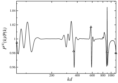
Fig. 3(a)

Fig. 3(b)

FIG. 3.: Test of our inversion method for a primordial spectrum (a) with a peak and a dip superposed on a scale-invariant spectrum and (b) with smoothly changing power-law index. (a) The top left panel shows $P^{(1)}(k)$ which is obtained from the first round of iteration. The solid curve is the original $P^{(1)}(k)$ which happens to have a very spiky dip at $kd\simeq 900$. We assume such a feature is spurious and remove it by simply cutting that part off and interpolating from the both sides, which is plotted by the dotted curve. The top right panel shows $P^{(2)}(k)$ and $P^{(4)}(k)$ together with the original (true) spectrum $P(k)$. The bottom panel shows $P^{(4)}(k)/P(k)$. The relative error is negligible except for regions near the singularities (marked by triangles) of the differential equation (16). Even near the singularities, the relative error is smaller than $\sim 4\%$. (b) In this case, we do not need to modify $P^{(1)}(k)$. The result reproduces the variation of the real spectrum well.

In the above, we assumed that the resolution of observations is limited to $\ell\leq\ell_{c}=1500$, which roughly corresponds to $kd\leq k_{c}d=1500$ in the primordial power spectrum. For our iterative procedure, however, we must assume the shape of the spectrum at scales $k>k_{c}$, because the contribution of modes at $k>k_{c}$ to the angular spectrum at $\ell<\ell_{c}$ is non-negligible. It becomes small enough only for $\ell\lesssim\ell_{c}/2$. Since there is no principle to determine the spectrum at $k>k_{c}$, we simply extrapolate the spectrum at $k<k_{c}$ to $k>k_{c}$ with a power-law form. This induces some errors in the angular spectrum at $\ell\gtrsim\ell_{c}/2$. In the case of the example shown in Fig. 3, the original spectrum is assumed to be scale-invariant at $k>k_{c}$ with the amplitude extrapolated from that at $k<k_{c}$. Hence we were able to recover the angular spectrum over the whole range up to $\ell=\ell_{c}$. In an actual application of our method, however, we must decide not to use $C^{\rm obs}_{\ell}$ at $\ell\gtrsim\ell_{c}/2$ as a criterion for the convergence.

IV Constraining cosmological parameters

In the previous section, we showed that the initial spectrum can be determined with a high precision. However we had to assume that the cosmological parameters, which are usually estimated from the CMB data, are exactly known by some other observations from the beginning. Here we examine consequences of the use of incorrect cosmological parameters in our procedure.

Naively, one might expect that our method is incapable of determining the cosmological parameters, since a different choice of cosmological parameters would simply give a spectrum that differs from the true spectrum. This is true in the rigorous sense. However, the very fact that the observed angular spectrum is used to determine the cosmological parameters indicates that there is not much freedom in varying cosmological parameters. In fact, if we use parameters that differ significantly from real values, very spiky features appear at the singularities of Eq. (16) in the reconstructed spectrum. Furthermore, depending on the direction of deviation from the real values, the reconstructed spectrum becomes negative in some regions of $k$, usually near the singularities, which never disappear by iteration.

As an example, Fig. 4 shows the reconstructed spectra for several values of $h$ and $\Omega_{b}$ when $C^{\rm obs}_{\ell}$ is given by a scale-invariant spectrum with $h=0.7$ and $\Omega_{b}=0.03$ in the flat CDM universe. As noted before, we may regard this case to describe a flat $\Lambda$CDM models with $\Omega_{\rm CDM}h^{2}=0.7$ as well. As for the $h$ dependence, spiky peaks appear at the singularities for larger values of $h$, while spiky dips appear for smaller values of $h$ and the dips become too deep to render the spectrum negative for $h\lesssim 0.65$. Therefore, the positivity condition of the spectrum severely constrains models with smaller values of $h$ and larger values of $\Omega_{b}$, while models with larger values of $h$ and smaller values of $\Omega_{b}$ can be also constrained unless there is a good reason to believe that locations of the spikes and the singularities should coincide.

V Conclusion

We have presented a method to solve the inversion problem of reconstructing the primordial curvature perturbation spectrum $P(k)$ solely from the CMB angular power spectrum $C_{\ell}$. In Paper I, we developed an inversion method by deriving a first order differential equation for $P(k)$ with its source term determined by $C_{\ell}$, but under the assumption of an infinitely thin LSS. In this paper, we improved it significantly by fully incorporating both the thickness of the LSS and the early ISW effect. This was made possible because of an empirical fact that the spectral ratio $b_{\ell}$ of the exact, full-numerically calculated angular spectrum $C^{\rm exact}_{\ell}$ to an approximate angular spectrum $C^{\rm app}_{\ell}$ using an analytic formula for the CMB multipoles (14) is relatively insensitive to variations of the shape of $P(k)$. This fact allowed us to apply the inversion method developed in Paper I iteratively to reconstruct $P(k)$. We have found the new method can recover the original spectrum accurately, to within relative errors of 4%, even in cases when there are distinct features like peaks and dips in the spectrum.

Our method, however, has a possible drawback that the inversion procedure can be performed only when the values of cosmological parameters are known. Therefore, we have also studied the effect of using the cosmological parameters that are different from their true values. We found that a small deviation from the true values results in the appearance of peaks and dips at the locations of singularities of the differential equation for $P(k)$, which can be easily judged as spurious. In particular, depending on the direction and the size of deviations, the spurious dips can become so deep that the positivity condition of $P(k)$ is violated there. Thus, contrary to our concern about the inversion method mentioned above, it may be regarded as an advantage in the sense that the cosmological parameters can be constrained severely with no regard to the shape of the initial spectrum. This is in accordance with a widely accepted assertion that the cosmological parameters can be determined from the heights and locations of peaks in the observed CMB spectrum. What is new is that we have not only justified this assertion qualitatively but also provided a means to quantify the level of its validity or limitations without any assumptions on the form of the primordial spectrum.

Finally, let us point out a couple of issues to be explored in future studies. First, we should investigate how observational errors on $C_{\ell}$ would be reflected to the reconstructed spectrum of $P(k)$. Second, our method in the present form can apply only to spatially flat universes. To make it more general, an extension to cases of spatially curved universes is necessary. In this respect, we may note the following. Apart from the geometrical effect of curved space that changes an angle sustaining a fixed distance on the LSS, we may adopt the small-angle approximation which allows us to use various flat space formulas. Hence, an extension to non-flat universes seems feasible enough, if not straightforward. Another issue is about the CMB polarization. Our method assume that the CMB spectrum is dominated by the scalar-type curvature perturbations. However, it has been argued that the CMB spectrum may contain a non-negligible contribution from tensor perturbations [15]. To identify the tensor contribution to the CMB spectrum, the CMB polarization spectrum plays a crucial role [16]. Hence, to complete the inversion problem, it is necessary to develop a formalism that utilizes both the temperature and polarization spectra to reconstruct both the scalar and tensor perturbation spectra simultaneously. These issues are currently under study.

FIG. 4.: The cosmological parameter dependence of the reconstructed spectrum. The real spectrum is scale-invariant with $h=0.7$ and $\Omega_{b}=0.03$ in the flat CDM universe. We plot the reconstructed spectra for $h=0.65$, $0.68$, $0.7$, $0.72$ and $0.75$, and $\Omega_{b}$=$0.02$, $0.03$ and $0.04$.

- [1] A. Balbi et al., Astrophys. J. 545, L1 (2000) [Erratum-ibid. 558, L145 (2001)] [arXiv:astro-ph/0005124]. A. H. Jaffe et al. [Boomerang Collaboration], Phys. Rev. Lett. 86, 3475 (2001) [arXiv:astro-ph/0007333]. A. E. Lange et al. [Boomerang Collaboration], Phys. Rev. D 63, 042001 (2001) [arXiv:astro-ph/0005004]. C. Pryke et al. Astrophys. J. 568, 46 (2002) [arXiv:astro-ph/0104490].
- [2] S. W. Hawking, Phys. Lett. 115B, 295 (1982); A. A. Starobinsky, ibid 117B, 175 (1982); A. H. Guth and S-Y. Pi, Phys. Rev. Lett. 49, 1110 (1982).
- [3] http://map.gsfc.nasa.gov/
- [4] http://astro.estec.esa.nl/SA-general/Projects/Planck/
- [5] A. D. Linde, Phys. Lett. B 158, 375 (1985). L. A. Kofman and A. D. Linde, Nucl. Phys. B 282, 555 (1987). J. Silk and M. S. Turner, Phys. Rev. D 35, 419 (1987). H. M. Hodges and G. R. Blumenthal, Phys. Rev. D 42, 3329 (1990). J. Yokoyama and Y. Suto, Astrophys. J. 379, 427 (1991); M. Sasaki and J. Yokoyama, Phys. Rev. D 44, 970 (1991). A. A. Starobinsky, JETP Lett. 55, 489 (1992); [Pisma Zh. Eksp. Teor. Fiz. 55 (1992) 477]; J. Yokoyama, Astron. Astrophys. 318, 673 (1997); J. Yokoyama, Phys. Rev. D 58, 083510 (1998);59, 107303 (1999); S. M. Leach and A. R. Liddle, Phys. Rev. D 63, 043508 (2001) [arXiv:astro-ph/0010082]; S. M. Leach, M. Sasaki, D. Wands and A. R. Liddle, Phys. Rev. D 64, 023512 (2001) [arXiv:astro-ph/0101406].
- [6] T. Souradeep et. al., astro-ph/9802262; Y. Wang, D. N. Spergel and M. A. Strauss, astro-ph/9812291; J. Lesgourgues, S. Prunet and D. Polarski, Mon. Not. Roy. Astron. Soc. 303, 45 (1999) [arXiv:astro-ph/9807020]; E. Gawiser, [arXiv:astro-ph/9807328]; Y. Wang, D. N. Spergel and M. A. Strauss, Astrophys. J. 510, 20 (1999) [arXiv:astro-ph/9802231]; S. Hannestad, Phys. Rev. D 63, 043009 (2001) [arXiv:astro-ph/0009296]; Y. Wang and G. Mathews, Astrophys. J. 573, 1 (2002) [arXiv:astro-ph/0011351];
- [7] A. Berera and P. A. Martin, Inverse Problems 15, 1393 (1999).
- [8] M. Tegmark and M. Zaldarriaga, Phys. Rev. D 66, 103508 (2002) [arXiv:astro-ph/0207047].
- [9] R.K. Sachs and A.M. Wolfe, Astrophys. J. 147, 73 (1967).
- [10] M. Matsumiya, M. Sasaki and J. Yokoyama, Phys. Rev. D 65, 083007 (2002) [arXiv:astro-ph/0111549].
- [11] W. Hu and N. Sugiyama, Astrophys. J. 444, 489 (1995).
- [12] H. Kodama and M. Sasaki, Prog. Theor. Phys. Suppl 78, 1 (1984)
- [13] cmbfast; http://physics.nyu.edu/matiasz/CMBFAST/cmbfast.html
- [14] W. Hu, M. Fukugita, M. Zaldarriaga and M. Tegmark, Astrophys. J. 549, 669 (2001) [arXiv:astro-ph/0006436].
- [15] A.A. Starobinsky, JETP Lett. 30, 682 (1979); V.A. Rubakov, M.V. Sazhin, and A.V. Veryaskin, Phys. Lett. 115B, 189 (1982). L.F. Abbott and M. Wise, Nucl. Phys. B244, 541 (1984); R. Crittenden, J.R. Bond, R.L. Davis, G. Efstathiou, and P.J. Steinhardt, Phys. Rev. Lett. 71, 324 (1993).
- [16] A.G. Polnarev, Soviet Astronomy, 29, 607 (1985); R. Crittenden, R.L. Davis, and P.J. Steinhardt, Astrophys.J. 417, L13-L16 (1993);