CN abundance variations on the main sequence of 47 Tuc

Abstract

We report on a deep spectroscopic survey for star-to-star CN variations along the main sequence (MS) of the globular cluster 47 Tuc with ESO’s VLT. We find a significant bimodal distribution in the $\rm{S}(3839)$ index for main-sequence stars in the mass range of $\sim 0.85$ to $0.65$ M_⊙ , or from the main-sequence turn-off down to $\sim 2.5$ mag below the main sequence turn-off. An anti-correlation of CN and CH is evident on the MS. The result is discussed in the context of the ability of faint MS stars to alter their surface composition through internal evolutionary effects. We argue against internal stellar evolution as the only origin for the abundance spread in 47 Tuc; an external origin such as pollution seems to be more likely.

1 Introduction

Globular clusters (GCs) are well suited to the study of ancient star formation and the evolution of low-mass stars. In standard formation scenarios all stars of a GC formed at the same time from a single proto cloud; as a consequence all stars within a cluster should have the same age and the same initial chemical composition. Indeed, within many globular clusters the star-to-star iron abundance spread is smaller than typical (spectroscopic or photometric) measurement errors (e.g., as reviewed by Suntzeff 1993, or in recent work by Gratton et al. 2001). Nevertheless, detailed studies have revealed that there are significant star-to-star abundance variations of certain light elements including sodium, aluminium, carbon, nitrogen, and oxygen in globular clusters (e.g., the review by Kraft 1994). One of the first discoveries of chemical inhomogeneities in GCs was made by Osborn (1971), who found two red giant stars in M10 and M5 to have enhanced CN molecular absorption strengths compared to other stars in these clusters.

The first detailed studies of the abundance spread phenomenon concentrated on the brightest stars at the tip of the red giant branch (RGB); increasing telescope size and improved instruments have allowed investigation of the chemical compositions of stars along the RGB down to the subgiant branch (SGB) (e.g., Bell et al. 1983, 1984; Hesser et al. 1984; Smith et al. 1989; Suntzeff & Smith 1991; Briley et al. 1992; Cohen, Briley, & Stetson 2002). Even the main sequence turn-off (MSTO) region of a few nearby GCs has been reached (Hesser, 1978; Briley et al., 1991, 1994; Suntzeff & Smith, 1991; Cannon et al., 1998; Cohen, 1999a, b; Briley & Cohen, 2001; Gratton et al., 2001). The main result of all these efforts in the last thirty years is the discovery of abundance variations in some GCs along the whole stellar evolutionary sequence from the RGB to the SGB and even to below the MSTO. Some of the better studied examples of globular clusters with abundance variations are 47 Tuc, M13, and M3.

The ultimate tool for studying the chemical compositions of GC stars is high-resolution spectroscopy of element absorption lines. Unfortunately, for stars near the MSTO of globular clusters this approach requires extremely long exposure times even with the present day 10-meter-class telescopes. However, the study of absorption bands produced by molecules can serve as a useful tool to investigate abundance variations even with moderate resolution spectra. For example, the broad CN and CH absorption features at $3883$ Å and $4300$ Å respectively are measurable for faint stars at the limits of large telescopes by either medium-resolution spectroscopy or narrow-band photometry.

To investigate the origin of abundance inhomogeneities in globular clusters, we have performed the deepest survey to date of CN band absorption in main sequence stars of the globular cluster 47 Tuc. In this paper we report on our observations with the Very Large Telescope (VLT), which has resulted in the detection of significant star-to-star differences in the CN abundance $2.5$ mag below the MSTO (i.e. V=$21.5$ mag) of 47 Tuc. In Sections 2 & 3 we briefly review current scenarios that could explain abundance spreads in GCs and describe earlier work on 47 Tuc. Sections 4 & 5 describe our observations and the data analysis. Our conclusions are presented in Section 6.

2 Scenarios for Abundance Inhomogeneities in Globular Clusters

Although the problem of abundance inhomogeneities, especially in the CN molecule, within globular clusters was recognized over thirty years ago, their origin is still unresolved. Over these thirty years three scenarios have received considerable discussion in the literature: (i) abundance changes produced internally by the evolution of GC stars, (ii) GC self-pollution, and (iii) primordial inhomogeneities or cluster self-enrichment. An excellent review of these scenarios can be found in Cannon et al. (1998), whose arguments we summarize here.

Stellar Evolution

If all stars in a globular cluster started with the same initial chemical composition, the surface abundances of many of them evidently have since changed by varying amounts during their subsequent evolution. In the stellar evolution scenario CNO-cycle processed material from the interior of hydrogen-burning stars is dredged up (e.g, by rotational mixing) to the stellar surface. The efficiency of this dredge up is reflected by changes in the surface chemical composition. This scenario can explain why chemical inhomogeneities are generally found in the CNO elements, but not in the iron-peak elements. Although according to conventional stellar evolution models the dredge up of processed material happens only on the RGB, CN variations are evident along the RGB, SGB, and at the MSTO of a number of globular clusters such as 47 Tuc, M71, and M5, e.g., Hesser (1978); Hesser & Bell (1980); Cannon et al. (1998); Cohen (1999a); Cohen, Briley, & Stetson (2002). As such, it is not currently possible to account for the luminosity behaviour of CN variations in GCs by a stellar evolution scenario. In many clusters the CN band strengths at a given stellar luminosity show a bimodal distribution (see e.g., Norris 1987; Smith 1987); the reason why stellar evolution would routinely produce a bimodality rather than a more uniform distribution is not yet understood.

Self Pollution

Asymptotic giant branch (AGB) stars with masses of $\sim 5$ M_⊙ eject stellar winds that contain considerable CNO processed material (e.g., Ventura, D’Antona, Mazzitelli, & Gratton (2001)). Other types of stars such as planetary nebulae progenitors or novae could also eject CNO-enriched material. These stellar winds may be accreted by other stars, including the present day MSTO, SGB, and RGB stars. Stars that accreted such material would show different surface compositions than stars that accreted no material. If only the stellar surfaces were polluted, deep convective mixing during the evolution along the RGB should dilute the chemical inhomogeneities. This effect is not seen at least in the case of the nitrogen abundance, although the [C/Fe] abundance is found to decrease with luminosity on the RGB in some clusters such as M92 and M13 (Carbon et al., 1982; Suntzeff, 1981). Also, a bimodal abundance distribution might not be expected from such a phenomenon, but rather a range in the surface contamination.

Primordial variations

The assumption that all stars in a globular cluster had the same chemical composition from the very beginning may not necessarily be true. For instance, two molecular clouds of different chemical composition could have merged and formed a globular cluster. If the gas was not mixed, stars would reflect the chemical composition of one or the other cloud. Here, a bimodal distribution could be explained. An imperfect merging of the gas clouds would lead to a range of abundances. Also, the first supernovae during the star forming epoch of a GC may have polluted the parent molecular cloud. Stars that formed after these events would be enriched in a variety of elements. These two primordial scenarios may explain abundance variations in the CNO elements, but they lack an easy explanation of the chemical homogeneity of the iron-peak elements. In a third “primordial” scenario two globular clusters experienced a collision and merged after they had completed their star formation. The result would be a bimodal abundance distribution, but again the homogeneity of the iron-peak and other heavy elements is a problem.

3 The Globular Cluster 47 Tuc

The globular cluster 47 Tuc is a very attractive object for a detailed chemical investigation. It has a distance of only $4.5$ kpc and it is after $\omega$ Cen the second-brightest cluster ($M_{V}=-9.4$ mag) in the Milky Way. Due to a tidal radius of $47.25^{\prime}$ it is quite an extended object on the sky. The intermediate metallicity of the cluster RGB stars ([Fe/H]=$-0.7$ dex) makes the formation of CN molecules in their atmospheres more efficient than in metal-poorer GC giants. Not surprisingly, a number of studies of CN abundance variations in 47 Tuc have been carried out. In one of the earliest studies McClure & Osborn (1974) found star-to-star differences in the DDO C(41-42) CN index. The distribution of CN band absorption strengths at a given point on the RGB was shown to have a bimodal signature by Norris & Freeman (1979), with there being indications of an anticorrelation between CN and CH band strengths (Norris, Freeman, & Da Costa, 1984). The main results from studies in the last 30 years show CN variations along the RGB of 47 Tuc down to the MSTO. In the latest large photometric narrowband filter survey of 47 Tuc, Briley (1997) verified the existence of a bimodal distribution of CN band strengths, with a radial gradient in the relative fraction of stars with strong and weak CN bands; in the inner part of the cluster there is a higher fraction of stars with strong CN absorption than in the outer parts. The existence of this gradient had been first noted by Norris & Freeman (1979), and further documented by Paltoglou (1990). References to additional studies can be found in Briley (1997).

The deepest CN survey done in 47 Tuc so far (and in GCs in general) extends to one magnitude below the MSTO (Cannon et al., 1998). These authors pursued deep spectroscopic work at the limits of a 4m-class telescope. They showed that the bimodal distribution of CN band strengths still exists on the upper main sequence. With the recent availability of 8 to 10-meter-class telescopes and with the capability of multi-object spectroscopy, large samples of stars on the fainter main sequence now become accessible for chemical abundance studies. The investigation of chemical inhomogeneities on the fainter main sequence can contribute new evidence for or against the various scenarios described above.

3.1 New information on the main sequence

In the evolutionary scenario of GC abundance variations all stars in a cluster started with the same initial chemical composition; internal evolutionary effects like deep mixing changed the star’s surface composition at a later date. To change the surface element abundances, two mechanisms are required: (i) a nuclear process must change the abundance of a certain element (in the case of the CNO process the ratio of the elements C, N, and O would be altered), and (ii) some interior mass transport mechanism(s) must dredge up the processed material to the stellar envelope. In this study we concentrate on abundance variations in the C and N elements since they can easily be detected spectroscopically by variations in the CN bands.

In the low-mass stars on the main sequence of globular clusters the pp-chain is the dominant process to produce nuclear energy in the stellar core. In addition the CNO process is contributing to the total energy output. Although the CNO cycle is a catalytic process, it can alter the abundance ratios of the elements involved due to the different time-scales of the various reactions in this cycle. Especially the nitrogen content increases at the cost of carbon and oxygen; the sum of C+N+O remains constant. The efficiency of the CNO process depends strongly on the temperature; therefore this cycle is the dominant nuclear process in young massive main sequence stars, but its contribution to the energy output is marginal for stars of a solar mass and below. According to stellar models globular cluster stars at the upper main sequence with masses of $\sim 0.8$ M_⊙ should not support deep mixing processes (the convective envelope being relatively shallow at least in terms of the contained mass) so that the stellar evolution scenario seems to fail to account for observed CN variations at the MSTO. Additionally, mixing processes would add fresh fuel to the hydrogen burning cores of the MS stars that would affect the lifetime of their core-burning phase. As pointed out in, e.g., Cannon et al. (1998), no such effect can be seen in 47 Tuc. Nevertheless, the understanding of deep mixing or other material transportation processes is still incomplete and other mechanisms like diffusion should still be taken into account.

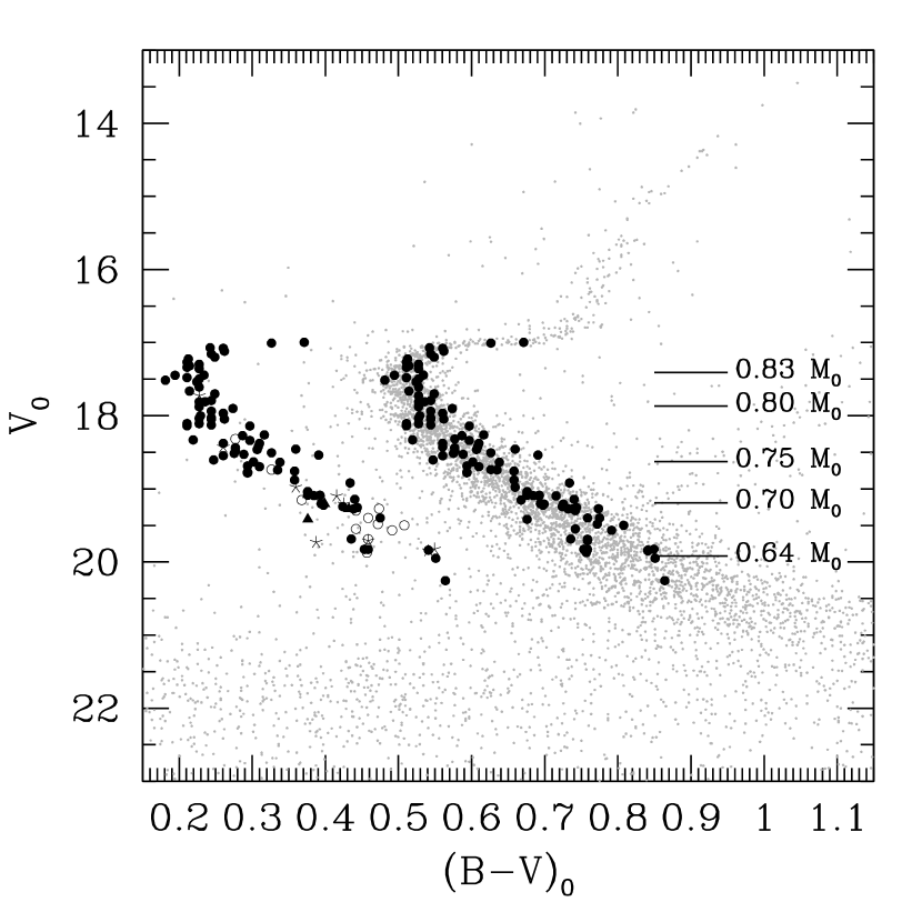
Figure 1: Color magnitude diagram of 47 Tuc based on WFI observations. All program stars are plotted on the main sequence with filled dots. Based on isochrones for $Z=0.004$ and an age of 14 Gyr (Girardi, Bressan, Bertelli, & Chiosi, 2000) we show the stellar masses at various points along the main sequence. For better visibility, all program stars are plotted again with an offset of $0.3$ mag in (B-V). Stars with clean CN measurements are plotted with filled circles (quality=”0”), while ambiguous measurements (quality= “1”) are indicated by open circles. Four cluster non-members, that are possibly SMC giants, are marked with triangles. Program stars with unreliable spectroscopy are marked by asterisks (quality=“2”).

Turn-off stars in 47 Tuc have masses of $0.85$ M_⊙ (see Fig 1). Cannon et al. (1998) showed that stars at the turn-off and below down to a magnitude of $V=18.6$ mag or a mass of $\sim 0.75$ M_⊙ exhibit CN abundance differences. In our study, we have measured stars with magnitudes down to $V=20$, or 2.5 mag below the MSTO, which have masses around $0.65$ M_⊙ (Fig. 1). The (model-dependent) core temperature of these stars is $\log(T_{c})\sim 7.10$ at the MSTO and $\log(T_{c})\sim 7.01$ for the fainter stars. These stellar parameters were taken from isochrones for a metallicity of $Z=0.004$ and an age of $14$ Gyr (Girardi, Bressan, Bertelli, & Chiosi, 2000). Due to the strong dependence of the CNO cycle energy production rate $\epsilon_{CNO}$ on the temperature ($\epsilon_{CNO}\propto T^{17}$), the contribution of the CNO cycle relative to the energy production by the pp-chain ($\epsilon_{pp}\propto T^{6}$) will be reduced by a factor of approximately ten in the fainter stars. This estimate is based on the decreased core temperature only and does not account for a decreasing core density. Therefore the CNO cycle efficiency in stars $2.5$ mag below the MSTO is suppressed by at least this factor of ten. If hydrogen-burning products could be dredged up to the surface, the amount of CNO processed material that could lead to CN variations would also be reduced by a factor of at least ten for the fainter stars.

This simple calculation can be summarized in the following statement: along the main sequence the production rate of N due to the CNO cycle becomes completely suppressed for the lower mass stars with masses of $\sim 0.65$ M_⊙ . If there is still some scatter in the CN content between faint stars along the MS, internal stellar evolution cannot explain this scatter because there is no internal CNO-process working to change the ratio of the CNO elements, and external processes (outside a given star) must have played an important role. If the abundance spread disappears among the fainter stars, this would be clear evidence for internal mixing processes as the origin of the CN abundance riddle. Measurements of the CN content of main sequence stars can therefore distinguish between the internal evolutionary scenario of CN variations and external scenarios. However, CN measurements alone cannot distinguish between different external scenarios. The main sequence study of Cannon et al. (1998) extends to a mass of $\sim 0.75$ M_⊙ . At this mass, the CNO process efficiency is reduced by only a factor of $\sim 3$. Surveying CN bands at even lower masses can greatly strengthen the constraints placed on the stellar evolution scenario by way of the above CNO-cycle efficiency argument.

4 Data and Reduction

4.1 Observations

Target selection from WFI imaging

Candidate stars in 47 Tuc for spectroscopy with the VLT of the European Southern Observatory (ESO) at Cerro Paranal, Chile, were chosen from CCD images of the cluster. In September 2000 we observed 47 Tuc with the MPG/ESO 2.2-m telescope at La Silla, Chile, using the Wide Field Imager (WFI) (Baade et al., 1998) with Johnson B and V filters. The exposure times were $3\times 300$ s in each filter. Conditions were non-photometric with a seeing of $1.5^{\prime\prime}$. The WFI offers a field of view (FoV) of $34$ arcmin² and consists of a mosaic of eight $4096\times 2048$ CCDs. The WFI was centered on the globular cluster. The radius of the FoV is $\sim 0.8^{\circ}$, which is approximately half the tidal radius of 47 Tuc. The basic processing of the raw CCD frames was done using the tasks esowfi and mscred in IRAF. To facilitate proper sky subtraction and to reduce the incidence of blended images we decided to only select stars in the outer, less-crowded regions of 47 Tuc for the follow-up spectroscopy. We therefore concentrated on chip #1 of the CCD mosaic (at the north-east corner of the FoV) to define the sample of spectroscopy candidates. With chip #1 we sample a radial coverage from $8^{\prime}$ to $25^{\prime}$, or $0.3$ to $0.5$ tidal radii. For the selected chip we performed PSF photometry using the DAOPHOT (Stetson, 1992) implementation in IRAF. Since the observations were obtained under non-photometric conditions and no local standard stars are available in the area covered by chip #1, we matched the observed MS and the SGB to fiducial lines published by Hesser et al. (1987). The calibrated photometry was dereddened assuming $E(B-V)=0.04$ (Harris, 1996). The resulting, dereddened color-magnitude diagram is shown in Fig. 1.

Spectroscopy with the VLT/FORS2/MXU

The goal of our spectroscopic observations was to measure the strengths of the $3883$ Å and $4215$Å CN absorption bands. We used the Focal Reducer and Low Dispersion Spectrograph 2 (FORS2) at the ESO VLT. FORS2 is equipped with a mask exchange unit (MXU) which allows multi-slit spectroscopy with freely defined metal slit masks and a FoV of $6.8\times 6.8$ arcmin². We defined three slit masks with the FORS instrument mask simulator (FIMS) software package provided by ESO. The positions of the program stars were determined on CCD images that were obtained at the FORS/MXU. The exposure time for the preimages was $45$ seconds with a V filter. The slit width on the masks was fixed to $1\,^{\prime\prime}$ and the slit length was chosen to be at least $8\,^{\prime\prime}$ to allow for local sky subtraction. Typically 35 slits were fitted onto one mask. In some cases two stars could be observed with one slit. We selected the grating B600 with a dispersion of $50$ Å mm^-1 or $1.2$ Å pixel^-1. In combination with the $1\,^{\prime\prime}$ slit width this results in a nominal spectral resolution of 815, or a line width of $\leq 5$ Å. The actual spectral coverage depends on the location of a star on the mask, but we took care to cover at least the range $3800$ Å to $5500$ Å. All program stars are listed in Table 1. The observations were carried out in service mode between 2001 July 18 and 2001 July 26. Each mask configuration was observed four times with exposure durations of $2925$ s each, leading to a total exposure time of 3.25 hours per mask. The seeing conditions were almost always better than $1\,^{\prime\prime}$ according to our specification for the service observations. Additionally, bias, flat field, and wavelength calibration observations were obtained.

4.2 Data reduction

All data were reduced using the ccdred and specred packages under IRAF. First all frames were overscan and bias corrected. The flat fields for each night and mask were stacked. Since each slit mask was observed four times and the alignment of the frames was excellent, we coadded the four frames for a given slit mask with cosmic ray rejection enabled. The resulting frames were almost free of cosmic rays. For further analysis we extracted the area around each slit and treated the resulting spectra as single-slit observations. The wavelength-calibration images and flat fields were treated in the same manner. We fitted a tenth-order polynomial to the flat field images to correct for the continuum. The (separated) object spectra and arc images were flat-field calibrated with these continuum-corrected flat fields. The doslit task was used to wavelength calibrate, sky-subtract, and extract the stellar spectra. The wavelength solution from the HgCd arcs was fitted by a fourth-order spline. The typical rms of the wavelength calibration is on the order of $0.2$Å, which is expected at the given spectral resolution.

Spectral indices

We measure the strength of the CN absorption bands at $3883$ Å and $4215$ Å using spectral indices $\rm{S}(3839)$ and $\rm{S}(4142)$ similar to those of Norris & Freeman (1979); Norris et al. (1981). These indices basically quantify the CN content of the atmospheres of red giant stars. Unfortunately, the main sequence stars we are considering here have strong hydrogen lines in the region of the $\rm{S}(3839)$ spectral index. We therefore modify this index according to Cohen (1999a) to exclude these hydrogen lines. Additionally we quantify the CH molecular absorption at $4300$ Å using a CH(4300) index defined according to Cohen (1999a,b). As a check we additionally extract an HK index that measures the absorption strength of the Ca ii H+K lines. The index definitions are:

$$\rm{S}(3839) = -2.5\log{\frac{F_{3861-3884}}{F_{3894-3910}}}$$ (1)

$$\rm{S}(4142) = -2.5\log{\frac{F_{4120-4216}}{0.4\,F_{4055-4080}+0.6\,F_{4240-4280}}}$$ (2)

$$\rm{CH}(4300) = -2.5\log{\frac{F_{4285-4315}}{0.5\,F_{4240-4280}+0.5\,F_{4390-4460}}}$$ (3)

$$\rm{HK} = -2.5\log{\frac{F_{3910-4020}}{F_{4020-4130}}}$$ (4)

where $F_{3861-3884}$ for example is the summed spectral flux (in our case ADU counts) from $3861$Å to $3884$Å. Each index quantifies the absorption strength of a molecular band or atomic lines relative to a nearby pseudo-continuum. For stronger band absorption the index values increase.

The derived indices $\rm{S}(3839)$ and $\rm{S}(4142)$ are plotted versus the $(B-V)$ color of each star in the upper panels of Fig. 2 and Fig. 3. The formation efficiency of the CN molecule depends on the temperature, and therefore the indices can have a dependence on the color of the stars. For $\rm{S}(3839)$ the effect here is negligible. To correct for this effect in the $\rm{S}(4142)$ index, we assume a combination of two straight lines (see Fig. 3) as a lower envelope and subtract this fit from the data. A constant value (see Fig. 2) is subtracted from $\rm{S}(3839)$ such that the corrected values approximately equal zero for the CN-poor stars. The corrected CN indices will be referred to as $\delta$$\rm{S}(3839)$ and $\delta$$\rm{S}(4142)$ ; they are plotted versus the stellar V magnitudes in the lower panels of Fig. 2 and Fig. 3. The derived index values can be found in Table CN abundance variations on the main sequence of 47 Tuc. The plotted error bars are calculated assuming Poisson statistics in the flux summations.

To verify the reliability of the $\rm{S}(3839)$ index we visually classified the CN absorption strength for all stars into five classes. We found an excellent correlation between the $\rm{S}(3839)$ index value and our visual classification. We have assigned a ”quality” flag to the data for each star. Stars for which spectra show clean CN absorption bands with few noise imperfections and for which a reasonably confident CN classifications was felt to be obtainable have been assigned a data flag of “0”. In some cases, however, we could not judge a unique CN classification by eye, especially for a few faint stars near to the center of 47 Tuc. Such instances tend to occur when spectra have a low S/N or do not show consistent trends in the three main absorption features at 3860Å,3875Å, or 3889Å of the blue CN band. These stars may be blended with others (as suspected by their proximity to the cluster center) and are flagged with a “1” in Table CN abundance variations on the main sequence of 47 Tuc. Nevertheless, the stars in this quality class generally follow a relation between the visual classification and the measured $\rm{S}(3839)$ absorption strength. For a few stars the data reduction produced poor S/N spectra. This may probably be due to a misallignment of the slits. These stars are flagged by a “2” in Table CN abundance variations on the main sequence of 47 Tuc as poor quality spectra. In Figs. 2 and 3 stars for which the spectrum obtained is assigned to quality class “1” are plotted with open circles. Stars that did not permit visual classifications are not plotted.

4.3 Membership of program stars

Field star contamination

We estimate the expected number of galactic foreground stars in our 47 Tuc field. According to Ratnatunga & Bahcall (1985) the expected contamination by the Milky Way is $\sim 3.5$ field main sequence stars per arcmin² in a $2$ mag interval from $V=18$ to $V=20$ and a $0.5$ mag interval in $(B-V)$ centered on the main sequence fiducial. We selected our spectroscopy candidate stars from a $0.05$ mag wide region in (B-V) about the 47 Tuc main sequence over a luminosity range from $V\sim 17.5$ mag to $\sim 20$ mag. We used only a small fraction of the FoV of FORS for candidate star selection due to our contraints on the wavelength coverage. Per mask configuration an effective FoV is $\sim 6^{\prime}\times 2^{\prime}=12$ arcmin². The expected number of field stars in the field of view of our three slit masks is therefore $\text@frac{3.5\,\rm{stars/arcmin}^{2}}{\cdot 2\,\rm{mag}\cdot 0.5\,\rm{mag}}\cdot 2.5\,\rm{mag}\cdot 0.05\,\rm{mag}\cdot 3\,\rm{masks}\cdot 12\,\rm{arcmin}^{2}\sim 16\,\rm{stars}$. The number of stars observed in the FoV of three slitmasks and the selected part of the 47 Tuc main sequence is $\sim 2500$. In our sample of $115$ spectroscopic survey stars we therefore expect a total number of $\text@frac{115}{2500}\cdot 16\sim 1$ field star. We conclude that the contamination by galactic field stars that cannot be identified by their radial velocity has a negligible effect on our results and does not account for the CN bimodality seen within our sample of stars.

Contamination by the SMC

In the color magnitude diagram of 47 Tuc (Fig. 1) the RGB of the Small Magellanic Cloud (SMC) crosses the main sequence of 47 Tuc at a magnitude of $V\sim 20$ mag. The SMC has a radial velocity of $+163$ km s^-1, while the radial velocity of 47 Tuc is $-18$ km s^-1. We determined the radial velocities (RVs) of the observed stars by measurement of the center of the calcium H+K lines as well as the H$\delta$ absorption line. The typical rms of the RV measurement for a single star is of order $30$ km s^-1 to $40$ km s^-1. For the well-sampled spectra we expect an accuracy of $\sim\text@frac{c}{850}\times\text@frac{1}{10}=35$ km s^-1, which is in good agreement with the actual measured scatter. The rvidlines task in the rv package in IRAF was used to determine the centers of the absorption lines. We found four stars with notably different radial velocities from the rest of our sample; they have magnitudes from $V=19$ mag to $V=20.25$ mag. These stars (number 3206, 4592, 5296, and 6335 in Table 1) could be SMC members from their location in the CMD, but since they are among the fainter stars in our sample the measured RVs could be affected by errors.

4.4 A correlaton between CN absorption bands

As a diagnostic we plot $\delta$$\rm{S}(3839)$ vs. $\delta$$\rm{S}(4142)$ in Fig. 4. Again, stars having spectra with some ambiguities (quality class “1”) are plotted with open circles. The outstanding group of four stars at $\delta$$\rm{S}(3839)$ $\sim 0.08$ and $\delta$$\rm{S}(4142)$ $\sim 0.08$ (plotted with filled triangles) are the stars noted in Section 4.3 as having radial velocities well off the measured RV distribution of 47 Tuc and are probably not cluster members. Although there is scatter present, the correlation between the two CN indices stands out. The star at $\delta$$\rm{S}(3839)$ $=0.35$ and $\delta$$\rm{S}(4142)$ $=0.01$ that does not follow the correlation is the reddest SGB star (compare to Fig. 1). Since the $\delta$$\rm{S}(4142)$ index is less sensitive to CN abundance, and in any event correlates with $\delta$S(3839), we will concentrate on the $\delta$$\rm{S}(3839)$ index in the remainder of this study.

5 CN variations on the main sequence

In the lower panel of Fig. 2 the $\delta$$\rm{S}(3839)$ index is plotted versus the stellar V band magnitudes. A pronounced variation in the measured CN index across the whole luminosity range covered is obvious. Even more, the distribution of CN absorption strength is bimodal: stars seem to be either CN-strong or CN-weak. There might be a possible turn-over at the faint end of our sample, although this could be an effect of increasing measurement errors. Our data demonstrate that CN variations exist in 47 Tuc even 2.5 mag below the MSTO. The range of the CN variations becomes more evident for lower luminosities ($V\geq 18.5$), which is probably an effect of the decreasing surface temperature and therefore increased efficiency of molecule formation. Rose (1984) showed for a sample of nearby dwarf stars that from spectral type G0 to K the CN 3883 band strength steadily increases, with the metal-richer stars showing a steeper increase as a function of spectral type. The increasing amplitude of the bimodal CN distribution is also evident in the less sensitive $\delta$$\rm{S}(4142)$ index in Fig. 3 (lower panel). Note that this effect was not seen in the study of Cannon et al. (1998), which only extends to a magnitude of $V=18.6$ mag. At this luminosity the bifurcation of the CN band strength starts to increase. In Fig. 5 we show spectra of CN-strong and CN-weak stars in three luminosity bins. Differences in CN band absorption are clearly visible, which was also seen in Fig. 2. We wish to point out here that at the luminosity of V$\sim 19.25$ the CN-weak sample suffers from SMC field star contamination. The two faintest stars with good quality spectra have luminosities of $V=19.25$ mag. CN-weak stars fainter than this luminosity still have reliable spectra, albeit of more limited S/N. Nevertheless, a verification by additional observations appears appropriate.

5.1 A Test of the CN Bimodality

The bimodality of the CN absorption strength is an outstanding feature of the main sequence of 47 Tuc. A bimodal CN distribution has been reported previously for the RGB, the SGB and the turn-off region (e.g., Norris & Freeman 1979, Cannon et al. 1998, and references therein). In Fig. 6 we plot histograms of the CN band strength $\delta$$\rm{S}(3839)$ for magnitude ranges $V\leq 18.5$ mag and $V\geq 18.75$ mag. The thick line is a smoothed plot of the $\delta$$\rm{S}(3839)$ values, where each measurement was folded by a Gaussian having a width equal to the error bar. The division into two luminosity bins is motivated by the increased absorption strengths of CN-enriched stars fainter than $V=18.5$ mag. A histogram of the CN absorption strength of all stars would smear out the bimodality due to the different range in index values at different magnitudes.

We quantify the significance of this bimodality with a kmm-test (Ashman, Bird, & Zepf, 1994). For the bright and faint samples we obtain confidence levels of $99.996$ % and $99.999$ % respectively for the distributions to be bimodal. This is very significant (indeed, the significance for the faint sample reached the numerical accuracy of the program used to calculate it).

In order to double-check if the bimodal distribution of CN strength could be caused by observational effects or errors in the data reduction, we plot the Ca ii H+K index defined in equation (4) versus the stellar V magnitude in Fig. 7. Higher values of HK indicate stronger calcium absorption. No bifurcation as for the CN indices is apparent. In this plot we mark CN-rich and CN-poor stars with filled and open circles, respectively. Although there is no clear trend, CN-poor stars might tend to have higher HK absorption and vice versa, but this effect is within the errors of the index measurements. We conclude that there is no obvious effect in the data that could mimic the bimodal distribution in the CN absorption strengths.

5.2 The CN/CH anticorrelation

In 47 Tuc an anti-correlation between CN and CH absorption band strength was reported in earlier studies of red giants (Norris, Freeman, & Da Costa 1984; Briley et al. 1994, and references therein). Such an anti-correlation indicates that an enhancement of CN coincides with a decrease in CH, or with a depletion of carbon at the expense of nitrogen. Such an anti-correlation is expected if CN variations are caused by variable amounts of CNO cycle processing. If the CNO process only alters the ratio of the CNO elements, the sum C+N+O must stay constant. An increase of nitrogen at the cost of carbon would (to a certain limit) increase the CN abundance but decrease the absolute content of carbon. As a result, the formation of the CH molecule would be suppressed.

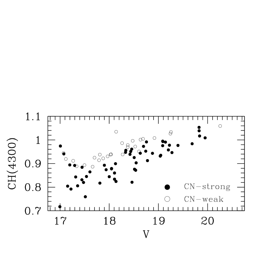
Figure 8: CH(4300) index plotted vs. the stellar magnitude for all stars with clean CN measurements (quality = “0”). Stars classified as CN-strong are plotted with filled circles; CN-weak stars are plotted with open cirles. Note that all CN-weak stars have strong CH absorption.

In Fig. 8 we plot the measured $\rm{CH}(4300)$  index versus the V band magnitude for all stars with good spectra (quality flag = “0”). Stars classified as CN-strong are plotted with filled circles, CN-weak stars are drawn with open circles. It is evident that stars with the strongest CH bands are weak in CN absorption. For the faintest stars in the sample ($V\geq 19.5$) this anti-correlation does not stand out clearly; we find that increasing absorption line strengths for these cooler stars affects the measurement of the comparison regions in the CH index.

6 Summary and Conclusions

Bimodal CN variations are detected in 47 Tuc among main sequence stars with masses down to 0.65 M_⊙ or $2.5$ mag below the MSTO. This extends earlier studies to stars that are nearly $1.5$ magnitudes fainter. There is an anticorrelation between the CN and CH absorption strengths on the main sequence of 47 Tuc.

6.1 External vs. evolutionary scenarios

In Section 3.1 we argued that for stars $2.5$ mag below the MSTO the CNO-cycle contribution is reduced by at least a factor of ten relative to the MSTO. Despite the fact that the faint stars in our sample should not be able to alter their chemical composition by themselves (by CNO-cycling plus mixing processes), they still show clear and significant star-to-star CN variations. Evidently the internal stellar evolution scenario seems be ruled out, at least as the only explanation for the CN-variation phenomenon in 47 Tuc. It is important to mention that from the tip of the RGB to the faint main sequence both (i) a bimodal CN distribution, and (ii) a CN/CH anti-correlation, are found in 47 Tuc. This suggests that the same effect causes the abundance spread from the tip of the RGB to the faint main sequence.

A caveat of our results is that an increased CN formation efficiency in the cooler atmospheres of the faint MS stars may compensate for any vanishing scatter in the CN content. The greater separation between CN-strong and CN-weak stars at the faint end of our sample in Fig. 2 may indicate that this effect is important. We plan to investigate temperature effects on CN formation in our sample by model atmosphere calculations in a subsequent paper. Additional observations would help to make our result more secure: for stars just one magnitude fainter than our sample the efficiency of the CNO-cycle relative to the pp-chain drops down by another factor of ten. Any diminution in the effects of internal evolution on the behaviour of CN would be even more evident among such stars than in our current study.

If internal stellar evolution can be ruled out, external scenarios remain to be discussed; either self-enrichment during the star forming episode of 47 Tuc or later self-pollution. However, early self-enrichment by high-mas stars is unlikely to produce only an imprint in the lighter elements like CNO. Self-pollution by high-mass AGB stars on the other hand could explain the lack of abundance variations in the heavy elements (e.g., as discussed in Cannon et al. (1998)). However, the bimodality of the CN band strength still needs to be explained, and the AGB-star enrichment/pollution scenario is not without other challenges (Denissenkov et al., 1997).

6.2 On the origin of the bimodality

Current scenarios can hardly explain all aspects of the bimodal distribution of CN absorption strengths in 47 Tuc or in other GCs. For example, it is not clear how internal pollution by AGB winds would lead to a bimodal abundance distribution. The measured bimodal CN distribution does not necessarily reflect a bimodal abundance spread: the distribution of CN absorption strengths reflects the true distribution of atomic abundances folded with the curve of growth (COG). It might be that all CN enhanced stars in 47 Tuc are polluted, but they would fall on the flat part of the COG. A continuum of atomic carbon and nitrogen abundances could therefore lead to more or less the same CN absorption strength at a given effective temperature. Such a “saturation” of the CN S(3839) band was proposed by Suntzeff (1981) and Langer (1985) to explain the bimodality of CN absorption in GC RGB stars. The similarity of CN absorption strength for the CN-rich stars might be explained by this saturation scenario, but the homogeneity of CN strength of the CN-poor stars remains unsolved: These stars would fall on the raising part of the COG; if pollution leads to a spread of abundances one would expect a continuum of CN absorption strength until the flat part of the COG is reached. This is not seen in the bimodal CN distribution of 47 Tuc. If indeed saturation happens for the CN-strong stars, then the CN-weak stars may represent the unpolluted, chemically homogeneous fraction of the cluster whose CN abundance falls on the raising part of the COG. Due to their chemical homogeneity they would have the same CN absorption strengths at a given effective temperature. The bimodal pollution mechanism still remains to be explained.

Binarity combined with AGB star pollution might be a solution: Only stars in binary systems would have experienced pollution by accreting the stellar winds of their evolving higher mass AGB companion. If single stars accreted only a negligible fraction of intracluster gas during the AGB contamination phase, the bimodality in the CN distribution would simply reflect the binary fraction in the globular cluster. If pollution in binary systems played an important role in GCs, one might also expect to find a significant number of CH stars. However, despite intense searches only a handful of CH stars have been found so far (e.g., Côté et al. 1997 and references therein).

6.3 Where is the polluting gas?

If self-pollution happened in globular clusters, should the polluting gas still be visible? The present-day amounts of gas in GCs appear to be extremely small and below the detection limits of classical approaches. Recently, ionized gas was detected in 47 Tuc from the measured radio dispersion of millisecond pulsar signals (Freire et al., 2001). The authors estimate the total gas mass in the cluster’s center to be roughly 0.1 M_⊙ . This amount is only a thousandth of the expected gas loss from stellar winds that should be ejected into the cluster between two passages through the Milky Way disk; therefore effective mechanisms must be at work to expel the gas. Freire et al. (2001) argue that only $0.5$% of the spin-down energy from the known millisecond pulsars in 47 Tuc would be required to expel this large an amount of gas from the cluster. Other mechanisms like novae and hot post-horizontal branch stars have also been under discussion as responsible for the mass loss from globular clusters. Smith (1999) showed that fast stellar winds ejected by main sequence stars can contribute to the gas loss. Therefore, at the present time pollution seems unlikely to happen. The crucial question then is whether during the era when intermediate mass stars evolved to AGB stars material from their stellar winds could have been retained in the globular cluster and have been re-accreted by other stars including the low-mass main-sequence stars that are observed at the present time. The mechanisms that are responsible for the ejection of stellar winds out of globular clusters were likely already at work in ancient times. Pulsars can form from stars with M=10 to 25 M_⊙ ; therefore many of them should have already formed by the time that 5 M_⊙ stars ejected their winds. Also main sequence star winds should have been present in ancient times. Nonetheless, Thoul et al. (2002) show that the overwhelmingly largest part of the gas from stellar winds is ejected within the first Gyr after the birth of a GC, so that the accretion scenario may be feasible in earlier times of cluster evolution.

6.4 Other support for external pollution scenarios

We have demonstrated that internal stellar evolution is unlikely to be the dominant origin of the CN variations in 47 Tuc. While primordial variations also have problems, the pollution scenario has its attractions, although it remains unproven.

Recent work by other groups add strong arguments that external enrichment processes can cause chemical inhomogeneities in GCs: from high-resolution spectroscopy Gratton et al. (2001) found a Mg-Al anti-correlation among turn-off stars in NGC 6752. The core temperatures of turn-off stars are too low to allow the proton capture process to convert Mg to Al and cause this anti-correlation. The authors conclude that internal mixing scenarios cannot account for the chemical inhomogeneities in this globular cluster (which also exhibits a bimodal CN distribution on the RGB Norris et al. 1981). They propose external enrichment by AGB stars as the mechanism at work (see also Ventura, D’Antona, Mazzitelli, & Gratton 2001). In this regard, it is important to note that Briley et al. (1996) had earlier shown that Na abundance inhomogeneities exist among main sequence stars in 47 Tuc. Indeed, the relative behavior of CN-Na-Mg-Al has a rich literature that we have not delved into here. The review by Kraft (1994) provides a good introduction. Detailed abundance analysis of RGB stars in $\omega$ Cen has revealed imprints of supernova Type Ia enrichment processes (Pancino et al., 2002), but Cunha et al. 2002 argue against this enrichment mode. Furthermore, the mostly metal-poor $\omega$ Cen also contains a metal-rich stellar population (e.g., Pancino et al. 2000) and has consequently been proposed to be the core of a disrupted dwarf galaxy (e.g., Freeman 1993; Hughes & Wallerstein 2000; Gnedin et al. 2002). As such, it may be an atypical example of self-enrichment processes in a globular cluster.

The question of the origin of the polluting gas in 47 Tuc can be addressed by searching for the fingerprints of different enrichment processes: cluster self-enrichment by massive stars versus accretion of material ejected in winds from intermediate-mass stars. Do the CN-strong main sequence stars have abundance enhancements in the elements Na, Mg, and Al, which can be produced by proton-addition reactions in intermediate-mass red giants, or by carbon burning in even more massive stars? Do they show enhancements in the much heavier r- and s-process elements such as Ba and Sr? High resolution spectroscopy might provide answers to these questions.

Figure 2: The CN index $\rm{S}(3839)$ plotted against the B-V color of 47 Tuc main sequence stars (upper panel). We correct for a zeropoint such that CN-weak stars have a corrected index $\delta\rm{S}(3839)=0$. This corrected CN index is plotted in the lower panel versus the stellar V magnitude. Note the significant scatter in the $\delta$$\rm{S}(3839)$ index even for the faintest stars. For stars fainter than $V=17.5$ mag the separation between CN-strong and CN-weak stars is more than 0.2 in $\rm{S}(3839)$ and increases with inreasing magnitude. The distribution of CN-poor and CN-enhanced stars does not seem to be random but is bimodal. Symbols are the same as in Fig. 1.

Figure 3: Same as Fig. 2, but for the weaker CN band index $\rm{S}(4142)$ . Since a baseline to the $\rm{S}(4142)$ index exhibits a stronger dependency on the temperature we correct with a linear fit (the pair of solid lines). Note the increased bimodality for the fainter stars. Symbols are the same as in Fig. 1.

Figure 4: Comparison of the CN indices $\delta$$\rm{S}(3839)$ and $\delta$$\rm{S}(4142)$ . Both indices, which measure absorption by the same molecule, are well-correlated. Symbols are the same as in Fig. 1.

Figure 5: Demonstration of the different CN absorption band strengths at 3883Å (between the dashed lines). We show example spectra of CN-strong (thin lines) and CN-weak (thick lines) stars at three different V magnitudes. The stars plotted are #806, #3060, #4344, #5545, #5759, and #5809.

Figure 6: Distribution of the CN absorption strengths $\delta$$\rm{S}(3839)$ for stars brighter than $V=18.5$ mag (upper panel) and fainter than $V=18.75$ mag (lower panel). The histogram bars show absolute number counts. The thick line is an error-folded density plot of the $\delta$$\rm{S}(3839)$ distribution. The bimodality of the distributions stands out in both sub-samples.

Figure 7: Distribution of Ca ii H+K absorption strength as a check of the data reduction. No bimodality such as for the CN distribution is seen, but a very weak anti-correlation between the CN and HK absorption.

Table 1: Data for Program stars

ID	$\alpha_{2000}$			$\delta_{2000}$			$V$	$(B-V)$	$\delta$$\rm{S}(3839)$	$\delta$$\rm{S}(4142)$	$\rm{CH}(4300)$	HK	Flag
90	00	26	05.54	-71	58	30.50	19.567	0.791	0.062	0.032	1.057	0.614	1
94	00	26	12.36	-71	58	11.10	18.547	0.561	0.360	0.053	0.896	0.402	0
341	00	26	03.55	-72	01	13.10	17.447	0.494	0.159	0.026	0.879	0.379	0
596	00	26	05.55	-71	58	34.20	19.547	0.742	0.102	0.011	1.050	0.617	1
806	00	26	43.04	-71	56	15.50	19.224	0.697	0.415	0.102	0.969	0.538	0
977	00	26	04.52	-72	02	44.60	18.697	0.610	0.316	0.047	0.969	0.451	0
1152	00	26	10.13	-72	02	32.40	19.207	0.725	0.869	-0.035	0.893	0.697	2
1173	00	26	20.17	-71	52	12.50	17.662	0.514	0.030	-0.003	0.885	0.388	0
1304	00	26	15.29	-71	50	28.80	17.537	0.524	0.200	0.032	0.839	0.353	0
1329	00	26	33.55	-71	50	10.70	18.273	0.587	0.066	0.022	0.938	0.434	0
1351	00	26	50.58	-71	49	47.80	17.793	0.544	0.028	0.019	0.914	0.408	0
1366	00	26	16.10	-72	02	15.30	20.247	0.891	0.249	0.083	0.824	0.394	0
1462	00	25	59.22	-72	02	07.50	18.137	0.511	0.273	0.059	0.811	0.396	0
1498	00	26	55.20	-71	47	39.40	17.514	0.481	0.172	0.007	0.763	0.350	0
1587	00	25	58.24	-72	01	54.50	17.967	0.560	0.035	0.026	0.926	0.407	0
1675	00	26	10.83	-72	01	42.90	18.427	0.561	-0.124	-0.021	1.059	0.817	2
1833	00	26	04.95	-72	01	24.10	19.707	0.758	0.056	0.022	1.055	0.597	2
1890	00	26	03.53	-72	01	16.10	17.727	0.527	0.420	-0.002	0.919	27.031	2
1992	00	26	10.19	-72	01	03.10	18.687	0.593	0.163	0.018	1.007	0.466	0
2060	00	25	56.72	-72	00	53.80	18.047	0.544	0.221	0.051	0.870	0.389	0
2186	00	26	04.69	-72	00	38.90	18.777	0.594	0.399	0.092	0.897	0.466	0
2284	00	26	01.69	-72	00	26.30	19.827	0.759	0.559	0.121	1.027	0.605	0
2379	00	26	09.14	-72	00	15.60	18.331	0.519	0.285	0.035	0.943	0.424	0
2409	00	26	09.15	-72	00	11.90	17.077	0.561	0.265	0.040	0.937	0.451	0
2556	00	26	09.91	-71	59	51.20	19.097	0.693	0.095	0.009	1.048	0.583	1
2629	00	26	05.13	-71	59	41.50	18.037	0.527	0.042	0.008	0.939	0.416	0
2738	00	26	05.38	-71	59	29.00	19.837	0.841	0.538	0.111	1.008	0.631	0
2821	00	26	12.39	-71	59	16.00	19.037	0.676	0.467	0.110	0.916	0.499	0
2947	00	26	09.49	-71	59	00.00	18.477	0.577	0.071	0.012	0.999	0.482	0
3060	00	25	59.94	-71	58	45.80	17.337	0.511	0.038	0.019	0.887	0.376	0
3137	00	26	31.88	-71	58	33.10	17.071	0.542	0.042	0.017	0.944	0.401	0
3206	00	26	11.39	-71	58	22.50	19.417	0.676	0.091	0.090	0.862	0.434	0
3230	00	26	11.42	-71	58	19.60	18.977	0.660	0.098	0.177	-0.161	0.594	2
3343	00	26	28.31	-71	58	02.60	18.514	0.575	0.361	0.080	0.860	0.422	0
3371	00	26	10.95	-71	57	58.40	17.297	0.527	0.147	0.034	0.888	0.374	0
3394	00	26	29.74	-71	57	55.60	18.742	0.635	0.387	0.068	0.943	0.475	0
3456	00	26	10.89	-71	57	47.30	19.397	0.759	0.016	0.034	1.045	0.591	1
3521	00	26	28.20	-71	57	37.10	18.337	0.597	0.198	0.035	0.955	0.418	0
3522	00	26	34.72	-71	57	36.90	19.826	0.754	0.437	0.120	1.039	0.598	0
3532	00	26	05.67	-71	57	36.70	17.267	0.511	0.056	0.018	0.910	0.380	0
3631	00	26	00.64	-71	57	23.40	19.497	0.808	0.359	0.100	0.994	0.655	1
3701	00	26	04.00	-71	57	12.40	19.087	0.676	0.423	0.084	0.985	0.528	0
3769	00	26	00.29	-71	57	01.90	18.107	0.527	0.267	0.032	0.850	0.410	0
3797	00	26	35.15	-71	56	58.20	17.809	0.536	0.053	0.007	0.940	0.411	0
3823	00	26	35.60	-71	56	54.80	18.140	0.597	0.151	0.015	1.059	0.429	0
3853	00	26	06.92	-71	56	50.60	18.127	0.544	0.237	0.037	0.893	0.397	0
3872	00	26	42.89	-71	56	47.70	18.261	0.617	0.057	0.018	0.989	0.453	0
3929	00	26	02.24	-71	56	40.30	19.297	0.742	0.156	0.007	1.050	0.571	1
3942	00	26	23.93	-71	56	38.10	19.270	0.773	0.066	0.028	1.014	0.543	1
4014	00	26	11.53	-71	56	27.90	18.027	0.544	0.063	0.006	0.940	0.411	0
4019	00	26	30.36	-71	56	26.60	19.824	0.849	0.113	-0.001	1.019	0.595	2
4023	00	26	13.09	-71	56	26.50	19.482	0.772	0.465	0.109	0.983	0.548	1
4115	00	26	11.27	-71	56	12.60	17.877	0.527	0.058	0.016	0.919	0.420	0
4188	00	26	12.11	-71	56	03.10	19.687	0.758	0.150	0.040	1.054	0.723	1
4298	00	26	54.92	-71	55	44.30	18.422	0.608	0.287	0.068	0.928	0.444	0
4344	00	26	33.67	-71	55	37.70	17.607	0.527	0.150	0.035	0.859	0.383	0
4421	00	26	34.06	-71	55	26.00	18.631	0.602	0.376	0.066	0.934	0.461	0
4452	00	26	17.37	-71	55	21.80	18.605	0.547	0.017	-0.014	0.953	0.422	0
4465	00	26	17.62	-71	55	19.90	18.463	0.607	0.441	0.108	0.800	0.435	0
4521	00	26	33.71	-71	55	12.00	19.202	0.694	0.424	0.115	0.946	0.514	0
4554	00	26	36.04	-71	55	06.40	16.996	0.671	0.341	0.041	0.781	0.532	0
4592	00	26	47.32	-71	55	00.60	19.273	0.732	0.054	0.087	0.834	0.465	0
4600	00	26	42.57	-71	54	59.70	18.777	0.594	0.107	0.004	1.037	0.483	1
4643	00	26	54.87	-71	54	52.20	17.497	0.527	0.007	0.018	0.890	0.371	0
4707	00	26	46.78	-71	54	42.90	18.000	0.529	0.266	0.061	0.832	0.394	0
4790	00	26	56.83	-71	54	27.50	18.437	0.577	0.237	0.028	0.947	0.438	0
4877	00	26	46.37	-71	54	14.00	18.457	0.659	0.297	0.052	0.956	0.452	0
4936	00	26	53.02	-71	54	03.20	17.937	0.544	0.248	0.041	0.866	0.401	0
5049	00	26	50.13	-71	53	43.50	17.007	0.626	0.199	0.023	0.973	0.432	0
5146	00	26	54.38	-71	53	26.80	19.949	0.851	0.357	0.044	1.006	0.519	0
5154	00	26	48.22	-71	53	26.00	18.377	0.561	0.040	-0.004	0.973	0.413	0
5188	00	27	04.02	-71	53	18.70	17.357	0.527	0.181	0.054	0.795	0.359	0
5205	00	26	19.88	-71	53	16.60	17.222	0.513	0.231	0.058	0.775	0.371	0
5214	00	26	51.50	-71	53	13.20	19.731	0.688	0.388	4.746	0.799	0.401	0
5219	00	26	20.25	-71	53	13.50	18.528	0.589	0.026	0.005	0.971	0.468	0
5231	00	26	51.88	-71	53	10.60	18.737	0.626	0.445	0.113	1.024	0.552	1
5235	00	26	56.51	-71	53	09.80	19.847	0.841	0.172	-0.007	1.041	0.628	2
5237	00	26	31.91	-71	53	09.50	19.255	0.744	0.046	0.007	1.040	0.593	0
5253	00	26	36.09	-71	53	07.60	18.879	0.658	0.475	0.069	0.932	0.488	0
5261	00	26	21.88	-71	53	06.80	20.255	0.864	0.161	0.041	1.066	0.569	0
5296	00	27	15.20	-71	52	58.70	19.077	0.676	0.047	0.082	0.850	0.448	0
5299	00	26	23.93	-71	53	00.30	19.153	0.668	0.113	0.011	1.046	0.591	1
5342	00	27	03.51	-71	52	51.40	17.477	0.511	0.178	0.029	0.813	0.369	0
5381	00	26	54.82	-71	52	42.70	19.047	0.676	0.419	0.048	0.936	0.471	0
5402	00	26	35.43	-71	52	38.60	18.377	0.610	0.053	0.021	0.977	0.464	0
5538	00	27	02.38	-71	52	12.80	18.317	0.577	0.186	0.022	0.959	0.428	1
5545	00	26	35.31	-71	52	11.50	18.636	0.638	0.063	0.006	1.004	0.482	0
5547	00	26	52.68	-71	52	10.60	19.397	0.775	0.643	0.136	0.954	0.536	0
5587	00	26	44.72	-71	52	01.60	17.701	0.549	0.029	0.013	0.926	0.409	0
5653	00	26	30.71	-71	51	47.60	18.046	0.562	0.190	0.038	0.871	0.397	0
5665	00	26	33.74	-71	51	43.60	17.154	0.544	0.229	0.061	0.790	0.394	0
5759	00	26	14.33	-71	51	26.10	17.318	0.514	0.178	0.036	0.836	0.360	0
5809	00	26	48.71	-71	51	16.90	19.243	0.724	0.050	0.006	1.035	0.583	0
5836	00	26	35.80	-71	51	11.60	18.757	0.658	0.311	0.036	0.991	0.506	0
5942	00	26	52.82	-71	50	48.50	19.143	0.740	0.525	0.099	0.980	0.550	0
5950	00	26	33.32	-71	50	47.50	19.096	0.716	0.420	0.530	-0.000	-0.000	2
6043	00	26	48.02	-71	50	24.60	17.810	0.527	0.229	0.064	0.803	0.385	0
6047	00	26	51.54	-71	50	23.80	17.118	0.562	0.036	0.029	0.917	0.404	0
6220	00	26	39.76	-71	49	42.70	18.537	0.691	0.381	0.103	0.856	0.459	0
6248	00	26	52.04	-71	49	35.70	18.919	0.734	0.094	0.009	1.014	0.543	0
6264	00	26	40.87	-71	49	33.80	19.871	0.757	0.419	0.112	0.978	0.671	1
6335	00	27	02.56	-71	49	16.80	19.207	0.699	0.075	0.093	0.812	0.482	0
6380	00	26	50.93	-71	49	09.30	19.685	0.735	0.513	0.111	0.976	0.614	0
6452	00	26	48.80	-71	48	50.70	18.507	0.626	0.355	0.037	0.922	0.447	0
6455	00	26	58.61	-71	48	49.70	17.901	0.574	0.190	0.030	0.888	0.396	0
6537	00	26	32.22	-71	48	29.00	17.198	0.549	0.106	0.042	0.887	0.391	0
6591	00	26	55.56	-71	48	14.60	17.444	0.534	0.186	0.034	0.823	0.366	0
6622	00	27	09.57	-71	48	04.80	21.893	0.219	0.071	-0.039	0.729	0.272	2
6641	00	27	13.08	-71	48	00.70	19.275	0.739	0.522	0.106	0.931	0.583	0
6648	00	26	45.61	-71	47	59.50	19.091	0.684	0.505	0.088	0.980	0.507	0
6723	00	26	48.58	-71	47	39.90	19.086	0.693	0.543	0.056	0.973	0.538	0

Note. — Qualityflag: 0=good quality spectra; 1=some ambiguities; 2=poor quality spectra - unreliable.

References

- Arnold (1996) Arnold, S.F. 1996, Mathematical Statistics (Prentice-Hall, England Cliffs, NJ), p.386
- Ashman, Bird, & Zepf (1994) Ashman, K. A., Bird, C. M., & Zepf, S. E. 1994, AJ, 108, 2348
- Baade et al. (1998) Baade, D., Meisenheimer, K., Iwert, O. et al. 1998, Messenger, 93, 13
- Bell et al. (1983) Bell, R. A., Hesser, J. E., & Cannon, R. D. 1983, ApJ, 269, 580
- Bell et al. (1984) Bell, R. A., Hesser, J. E., & Cannon, R. D. 1984, ApJ, 283, 615
- Briley (1997) Briley, M. M. 1997, AJ, 114, 1051
- Briley et al. (1991) Briley, M. M., Hesser, J. E., & Bell, R. A. 1991, ApJ, 373, 482
- Briley et al. (1994) Briley, M. M., Hesser, J. E., Bell, R. A., Bolte, M., & Smith, G. H. 1994, AJ, 108, 2183
- Briley et al. (1992) Briley, M. M., Smith, G. H., Bell, R. A., Oke, J. B., & Hesser, J. E. 1992, ApJ, 387, 612
- Briley et al. (1996) Briley, M. M., Smith, V. V., Suntzeff, N. B., Lambert, D. L., Bell, R. A., & Hesser, J. E. 1996, Nature, 383, 604
- Briley & Cohen (2001) Briley, M. M., & Cohen, J. G. 2001, AJ, 122, 242
- Cannon et al. (1998) Cannon, R. D., Croke, B. F. W., Bell, R. A., Hesser, J. E., & Stathakis, R. A. 1998, MNRAS, 298, 601
- Carbon et al. (1982) Carbon, D. F., Romanishin, W., Langer, G. E., Butler, D., Kemper, E., Trefzger, C. F., Kraft, R. P., & Suntzeff, N. B. 1982, ApJS, 49, 207
- Chun & Freeman (1978) Chun, M. S. & Freeman, K. C. 1978, AJ, 83, 376
- Cohen (1999a) Cohen, J. G. 1999a, AJ, 117, 2428
- Cohen (1999b) Cohen, J. G. 1999b, AJ, 117, 2434
- Cohen, Briley, & Stetson (2002) Cohen, J. G., Briley, M. M., & Stetson, P. B. 2002, AJ, 123, 2525
- Côté et al. (1997) Côté, P., Hanes, D. A., McLaughlin, D. E., Bridges, T. J., Hesser, J. E., & Harris, G. L. H. 1997, ApJ, 476, L15
- Cunha et al. (2002) Cunha, K., Smith, V. V., Suntzeff, N. B., Norris, J. E., Da Costa, G. S., & Plez, B. 2002, AJ, 124, 379
- Denissenkov et al. (1997) Denissenkov, P. A., Weiss, A., & Wagenhuber, J. 1997, A&A, 320, 115
- Freeman (1993) Freeman, K. C. 1993, in Galactic Bulges, IAU Symp 153, ed. H. Dejonghe & H. J. Habing (Dordrecht: Kluwer), p. 263
- Freire et al. (2001) Freire, P. C., Kramer, M., Lyne, A. G., Camilo, F., Manchester, R. N., & D’Amico, N. 2001,ApJ, 557, L105
- Girardi, Bressan, Bertelli, & Chiosi (2000) Girardi, L., Bressan, A., Bertelli, G., & Chiosi, C. 2000, A&AS, 141, 371
- Gnedin et al. (2002) Gnedin, O. Y., Zhao, H. S., Pringle, J. E., Fall, S. M., Livio, M., & Meylan, G. 2002, ApJ, 568, L23
- Gratton et al. (2001) Gratton, R. G. et al. 2001, A&A, 369, 87
- Harbeck et al. (2001) Harbeck, D. et al. 2001, AJ, 122, 3092
- Harris (1996) Harris, W. E. 1996, AJ, 112, 1487
- Hesser (1978) Hesser, J. E. 1978, ApJ, 223, L117
- Hesser & Bell (1980) Hesser, J. E. & Bell, R. A. 1980, ApJ, 238, L149
- Hesser et al. (1984) Hesser, J. E., Harris, G. L. H., Bell, R. A., & Cannon, R. D. 1984, in Observational Tests of the Stellar Evolution Theory, IAU Symp. 105, eds. A. Maeder & A. Renzini. (Dordrecht: Reidel), p. 139
- Hesser et al. (1987) Hesser, J. E., Harris, W. E., Vandenberg, D. A., Allwright, J. W. B., Shott, P., & Stetson, P. B. 1987, PASP, 99, 739
- Hughes & Wallerstein (2000) Hughes, J., & Wallerstein, G. 2000, AJ, 119, 1225
- Kraft (1994) Kraft, R. P. 1994, PASP, 106, 553
- Langer (1985) Langer, G. E. 1985, PASP, 97, 382
- McClure & Osborn (1974) McClure, R. D. & Osborn, W. 1974, ApJ, 189, 405
- Norris & Freeman (1979) Norris, J. & Freeman, K. C. 1979, ApJ, 230, L179
- Norris et al. (1981) Norris, J., Cottrell, P. L., Freeman, K. C., & Da Costa, G. S. 1981, ApJ, 244, 205
- Norris, Freeman, & Da Costa (1984) Norris, J., Freeman, K. C., & Da Costa, G. S. 1984, ApJ, 277, 615
- Norris (1987) Norris, J. 1987, ApJ, 313, 65
- Osborn (1971) Osborn, W. 1971, The Observatory, 91, 223
- Paltoglou (1990) Paltoglou, G. 1990, BAAS, 22, 1289
- Pancino et al. (2000) Pancino, E., Ferraro, F. R., Bellazzini, M., Piotto, G., & Zoccali, M. 2000, ApJ, 534, L83
- Pancino et al. (2002) Pancino, E., Pasquini, L., Hill, V., Ferraro, F. R., & Bellazzini, M. 2002, ApJ, 568, L101
- Ratnatunga & Bahcall (1985) Ratnatunga, K. U. & Bahcall, J. N. 1985, ApJS, 59, 63
- Rose (1984) Rose, J. A. 1984, AJ, 89, 1238
- Smith (1987) Smith, G. H. 1987, PASP, 99, 67
- Smith et al. (1989) Smith, G. H., Bell, R. A., & Hesser, J. E. 1989, ApJ, 341, 190
- Smith (1999) Smith, G. H. 1999, PASP, 111, 980
- Stetson (1992) Stetson, P.B. 1992, in ASP Conf. Ser. 25, Astronomical Data Analysis Software and Systems I, eds. D.M. Worrall, C. Biemesderfer, & J. Barnes (San Francisco: ASP), 297
- Suntzeff (1981) Suntzeff, N. B. 1981, ApJS, 47, 1
- Suntzeff & Smith (1991) Suntzeff, N. B., & Smith, V. V. 1991, ApJ, 381, 160
- Suntzeff (1993) Suntzeff, N. 1993, ASP Conf. Ser. 48: The Globular Cluster-Galaxy Connection, 167
- Thoul et al. (2002) Thoul, A., Jorissen, A., Goriely, S., Jehin, E., Magain, P., Noels, A., & Parmentier, G. 2002, A&A, 383, 491
- Ventura, D’Antona, Mazzitelli, & Gratton (2001) Ventura, P., D’Antona, F., Mazzitelli, I., & Gratton, R. 2001, ApJ, 550, L65