Measuring the Influence of Supernovae at High Redshift

Abstract

Supernovae play a large but poorly understood role in our attempts to explain the evolution of the baryonic universe. Numerous observations throughout astronomy cannot be explained if we neglect their influence, yet our quantitative understanding of the ways in which supernovae affect the universe remains remarkably poor. This is one of the most embarrassing gaps in our knowledge of the cosmos, and planned telescopes and surveys will probably not do much to fill it. The problem is that these surveys will be optimized to observe galaxies and intergalactic material independently of each other, while (in the author’s view) by far the best information will come from simultaneous surveys of galaxies and the intergalactic material (IGM) in their vicinity. Only this will show directly how galaxies affect their surroundings and provide a rough energy scale for supernova-driven winds. Redshifts $1\mathrel{\hbox{\hbox to0.0pt{\hbox{\lower 4.0pt\hbox{$\sim$}}\hss}\hbox{$<$}}}z\mathrel{\hbox{\hbox to0.0pt{\hbox{\lower 4.0pt\hbox{$\sim$}}\hss}\hbox{$<$}}}3$ are ideal for the joint galaxy/IGM surveys we advocate, because the comoving density of star formation is near its peak, because the Lyman-$\alpha$ forest is thin enough for QSO spectra to reveal the locations of the dominant metallic species, and because bright background QSOs are common. But a new UV-capable spectrograph in space will be required.

Harvard-Smithsonian Center for Astrophysics, 60 Garden St., Cambridge, MA 02138

1. Introduction

Fifteen years from now we will be awash in galaxies. 2dF, Sloan, and maybe a Sloan successor will have given us redshifts for more than a million galaxies in the nearby universe. DEEP and VVDS will have added $\sim 10^{5}$ galaxies out to redshift $z\sim 5$. NGST and 30m optical/IR telescopes on the ground may have detected thousands of galaxies to $z\mathrel{\hbox{\hbox to0.0pt{\hbox{\lower 4.0pt\hbox{$\sim$}}\hss}\hbox{$>$}}}10$—some of the first sources of light in the universe. These surveys and others will teach us a tremendous amount about galaxy and structure formation. Our communal efforts so far will seem little more than a prologue to the vast literature on galaxies that will exist in 15 years.

Nevertheless I suspect that one of the most fundamental questions in galaxy formation (and in all astronomy!) will remain largely unanswered. This is the role that supernovae played in shaping the baryonic universe. The influence of supernovae is thought to account for a wide range of observations throughout our field. The disruption of star-formation by supernova explosions is the favored explanation for why so few baryons are found in stars today (e.g., White & Rees 1978, Springel & Hernquist 2002). Numerical simulations cannot reproduce the large disk galaxies that we observe around us unless they include substantial heat input from supernovae (e.g., Weil, Eke, & Efstathiou 1998). The material between galaxies at high-redshift is hotter than would be expected if gravity and the background radiation field were the only sources of heating; another source, presumably supernovae, appears to be required (Cen & Bryan 2001). It is difficult to explain why the soft X-ray background is so faint and so dominated by AGN without asserting that supernovae blew apart dense clumps of baryons that would otherwise have produced copious free-free emission (e.g., Pen 1999). The shape of galaxy clusters’ X-ray temperature/luminosity relationship differs from naive expectations in a way that suggests that supernovae may have imparted $\sim 1$ keV of energy to each of the young universe’s nucleons (e.g., Kaiser 1991; Ponman, Cannon, & Navarro 1999).

These examples are only a few of many. We are unable to account for much of what we observe around us without invoking the indistinct notion of strong supernova “feedback,” and our understanding of the evolving universe will remain seriously incomplete until we comprehend quantitatively how this feedback works.

The standard picture is that the numerous supernova explosions in a young galaxy create an enormous blast-wave (or “wind”) that rips through the galaxy and lays waste to its surroundings. But working through the details of this picture remains challenging even after 30 years of theoretical studies. There are many complications, but the central problem is that we have little idea of the characteristic energy scale to associate with the blast-waves that supernovae drive. The energy released by a single supernova, $\sim 10^{51}$ erg, is known, but it is unclear how large a fraction of the energy released by supernova explosions is imparted to nascent winds. Much of it may be harmlessly radiated away by the dense gas it heats. Physical arguments and numerical simulations are at present incapable of estimating a priori the energy of a galaxy’s wind to within even an order of magnitude—and the energy of the winds is largely what determines how large an impact they have on the evolving baryonic universe. For this reason it is still unclear (e.g.) which sorts of galaxies were responsible for seeding the intergalactic medium with metals, or what effect blast-waves have on galaxy formation and evolution, or even whether realistic blast-waves would be physically capable of filling the large role that they are assigned in the standard lore.

Whether numerical calculations in 2017 will be able to reliably estimate the energy of galaxies’ winds from first principles is anyone’s guess, but in any case we will certainly want empirical support for the numerical results. Properties of galaxies (e.g., disk sizes) and of the IGM (e.g., metal content) are affected by the strength of supernova winds, and I can imagine convoluted and uncertain chains of reasoning that would provide an estimate the strength of winds from observations of one or the other; but surely the most straightforward way to estimate the strength of galaxies’ winds is to observe galaxies and the intergalactic medium simultaneously and see how much winds have disturbed galaxies’ surroundings. Winds lose energy as they climb out of galaxies’ potential wells and crash into nearby intergalactic matter, and a robust (if crude) measurement of the typical energy of galaxies’ winds can be obtained by seeing how far they are able to propagate. Simultaneous observations of galaxies and the intergalactic material that surrounds them are easy to obtain, at least in principle: one need only conduct a galaxy redshift survey in a field that contains background QSOs whose absorption spectra reveal the locations of HI and metals in the IGM. These sorts of observations, present and future, are the subject of my talk.

2. Current data

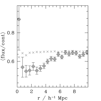
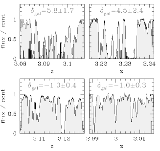
Figure 1.: Left: the mean Lyman-$\alpha$ transmissivity of the IGM as a function of comoving distance from Lyman-break galaxies. Points with error bars show our measurements; crosses show the result if we randomize the galaxy redshifts. Since Ly-$\alpha$ transmissivity decreases as the HI content of the IGM is increased, the plot shows that Lyman-break galaxies tend to be surrounded by large amounts of HI at comoving radii $1\mathrel{\hbox{\hbox to0.0pt{\hbox{\lower 4.0pt\hbox{$\sim$}}\hss}\hbox{$<$}}}r\mathrel{\hbox{\hbox to0.0pt{\hbox{\lower 4.0pt\hbox{$\sim$}}\hss}\hbox{$<$}}}5h^{-1}$ Mpc but little HI at smaller radii. Right: The HI content of the IGM along skewers through our two most significant galaxy overdensities (top) and underdensities (bottom). The shaded region shows the Ly-$\alpha$ absorption in the QSO spectrum; vertical bars mark the measured redshifts of galaxies, which are typically a few comoving Mpc away from the QSO’s line-of-sight. The overdensities, presumably young Abell clusters, contain large amounts of HI—a result consistent with the idea that gas between the galaxies has been roiled by supernova-driven winds. See Adelberger et al. (2002), Adelberger (2003).

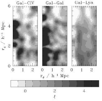
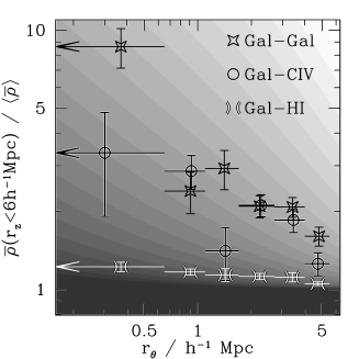
Figure 2.: Left: the two-dimensional correlation functions of galaxies with galaxies, with CIV absorption systems, and with Lyman-$\alpha$ transmissivity decrements. Distances along the line-of-sight ($r_{z}$) and along the plane of the sky ($r_{\theta}$) are comoving. The Ly-$\alpha$ panel was multiplied by $-10$ to make its structure visible. Right: a marginalization over redshift of the data in the left panel. Points with error bars are as labeled. Striations in the background show how this plot would appear if the unmarginalized density had the form $\rho(r)\propto 1+(r/r_{0})^{-1.6}$.

Figures 1 and 2 show examples of what one can learn about galaxies’ winds at high redshift from data that are currently available. These data, described more thoroughly in Adelberger et al. (2002), consist of measured redshifts for 431 Lyman-break galaxies in 6 fields at $z\sim 3$ together with high-resolution spectra of a bright background QSO in the middle of each field. The leftmost panel of Figure 1 shows the mean Lyman-$\alpha$ transmissivity of the IGM as a function of distance from Lyman-break galaxies at redshift $z\sim 3$. Increases in the HI content of the IGM lead to more Lyman-$\alpha$ absorption and hence to a lower Lyman-$\alpha$ transmissivity. (Here the IGM’s Lyman-$\alpha$ transmissivity at redshift $z$ is quantified as the ratio of observed flux in a QSO’s spectrum at wavelength $\lambda=(1+z)\lambda_{Ly\alpha}$ to the QSO’s expected flux if there were no absorption from the IGM.) The figure shows that as one approaches a Lyman-break galaxy from afar, the density of intergalactic HI at first begins to rise. This is in accord with the simple view that galaxies ought to be found where the density of matter (including HI) is highest. But at small separations ($r\mathrel{\hbox{\hbox to0.0pt{\hbox{\lower 4.0pt\hbox{$\sim$}}\hss}\hbox{$<$}}}0.5h^{-1}$ comoving Mpc) something else happens; intergalactic HI largely disappears. One interpretation is that the galaxies’ winds have largely driven away all material within this radius; the competing hypothesis that the galaxies’ light has ionized the HI is ruled out by the large size of region with lowered HI content (Adelberger et al. 2002).

The right panel of Figure 1 shows the difference between the neutral hydrogen content of the intergalactic medium in young galaxy clusters and in young voids. Far more neutral hydrogen is found in the young clusters. The trend appears stronger than would be expected solely from the fact that galaxy clusters ought to contain more matter of all sorts (Adelberger et al. 2002). A possible explanation is that the roiling of the young intracluster medium by galaxies’ blast-waves creates density inhomogeneities and increases hydrogen’s neutral fraction (Adelberger 2002, 2003).

If Mpc-scale winds are responsible for the HI results just discussed, one might expect to find an increase in the density of metals near galaxies. This appears to be the case, as can be shown in a variety of ways. Consider first the triptych in the left half of Figure 2. Shown are the two dimensional correlation functions of galaxies with galaxies, of galaxies with CIV absorption systems, and of galaxies with Ly-$\alpha$ transmissivity decrements. The panels show how the densities of HI, CIV, and other galaxies vary with spatial separation from a typical Lyman-break galaxy at redshift $z\sim 3$; one should imagine that the typical galaxy is at the origin and that the shadings indicate the amount of material at various angular and redshift separations. $\xi({\mathbf{r}})$ is defined so that the mean density at any separation ${\mathbf{r}}$ is $\rho({\mathbf{r}})=\langle\rho\rangle(1+\xi({\mathbf{r}}))$ with $\langle\rho\rangle$ the global mean. Positive values of $\xi$ correspond to overdensities, negative to underdensities. One may immediately see that the intergalactic medium near galaxies at $z\sim 3$ contains a large overdensity of CIV systems.

Now consider the right panel of Figure 2, which shows the same data marginalized in the redshift direction, $\bar{\rho}(r_{\theta},<r_{z})\propto\int_{0}^{r_{z}}dr_{z}^{\prime}\rho(r_{\theta},r_{z}^{\prime})$, where the marginalization helps remove dependence on redshift measurement errors or peculiar velocities. Contemplation of this figure reveals (a) that the ratio of CIV to HI density increases near galaxies, suggesting perhaps that the intergalactic metallicity is highest close to galaxies, and (b) that on large scales the galaxy-CIV cross-correlation function is similar to the galaxy-galaxy auto-correlation function, suggesting that CIV absorption systems and galaxies may be similar objects. Readers will find a slightly less glib discussion in Adelberger et al. (2002).

3. Ideal data

I will not pretend that the data just presented are entirely convincing. In fact the entire point of my talk is to advertise their inadequacy! Some might worry that the statistical significance of any one of these results is low, but that does not concern me much. The flaw is easily fixed; existing telescopes will shrink our error bars by a factor of a few in a relatively short time. I am more concerned with the fundamental limitations of the data. There are several. I will mention two.

Measuring the content of the IGM along a single skewer through the galaxy distribution can tell us something about the characteristic stalling radii of the winds, and hence about their typical energies, but it tells us almost nothing about their geometry. Are they (e.g.) isotropic or bipolar? This has significant implications but cannot be determined if the IGM is observed only along a single skewer. Ideally one would have several background QSOs whose light pierced each galaxy’s wind at a range of angles and impact parameters.

More serious is the fact that working at $z\mathrel{\hbox{\hbox to0.0pt{\hbox{\lower 4.0pt\hbox{$\sim$}}\hss}\hbox{$>$}}}3$ forces us to rely almost exclusively on the IGM’s CIV content as a proxy for its metal content. The density of CIV is not related in a simple way to the metal content of the IGM (see, e.g., Adelberger et al. 2002). Inferences about intergalactic metals based solely on CIV will always be somewhat suspect—to say the least. But metals are the most direct signature of supernovae , and measuring the dispersal of metals out of galaxies and into the IGM will be central to our attempts at understanding supernova-driven winds. Ideally one would be able to measure the density of several metallic species, not merely CIV. This would provide constraints on the ionization parameter and let one say something definitive about metallicity. The relative abundances of different elements would also (in principle) provide information about their nucleosynthetic origin. But the vast majority of the strongest absorption lines at intergalactic temperatures and densities have wavelengths similar to or shorter than Lyman-$\alpha$’s. This means that at redshifts $z\mathrel{\hbox{\hbox to0.0pt{\hbox{\lower 4.0pt\hbox{$\sim$}}\hss}\hbox{$>$}}}3$ they are buried in the thick Lyman-$\alpha$ forest and are extraordinarily difficult to detect. Only at redshifts $z\mathrel{\hbox{\hbox to0.0pt{\hbox{\lower 4.0pt\hbox{$\sim$}}\hss}\hbox{$<$}}}3$, where the decreasing density of the universe slows recombination and thins the forest, can these metallic absorption lines be straightforwardly found.

So this, then, is my picture of the ideal survey for quantifying empirically how supernova winds have affected the universe. Find a field with a very large number of QSOs at redshifts $1\mathrel{\hbox{\hbox to0.0pt{\hbox{\lower 4.0pt\hbox{$\sim$}}\hss}\hbox{$<$}}}z\mathrel{\hbox{\hbox to0.0pt{\hbox{\lower 4.0pt\hbox{$\sim$}}\hss}\hbox{$<$}}}3$ and obtain high-S:N, high-resolution spectra of each. (The upper redshift bound comes from our desire that several intergalactic metal lines be easily detectable, the lower bound from the fact that the comoving density of star-formation, and presumably the prevalence of powerful winds, declines rapidly at $z<1$.) Derive from the QSOs’ absorption lines a detailed picture of the distribution of HI and metals in the intergalactic medium. Conduct a redshift survey of galaxies at $1\mathrel{\hbox{\hbox to0.0pt{\hbox{\lower 4.0pt\hbox{$\sim$}}\hss}\hbox{$<$}}}z\mathrel{\hbox{\hbox to0.0pt{\hbox{\lower 4.0pt\hbox{$\sim$}}\hss}\hbox{$<$}}}3$ in the same field and discover where star-forming galaxies lie amid the jumbled distribution of intergalactic matter. Then compare the relative spatial distributions of galaxies and intergalactic material. To the extent that galaxies send winds into their surroundings, one should find that the intergalactic medium near them is disturbed. Perhaps most of the intergalactic gas will have been driven away; perhaps large amounts of metals will be found at the winds’ stalling radii. In any case, one should be able to answer the following questions (and others): What fraction of the energy released by supernovae appears to have been imparted to galaxies’ winds? What sorts of galaxies drive winds? Are winds from dwarf galaxies really the most important, as many have argued? Are the winds more isotropic or bipolar? What is their dominant effect on the the large fraction of the universe’s baryons that lies outside of galaxies? And so on.

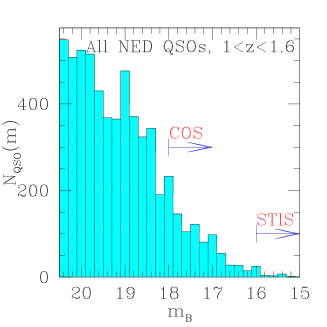
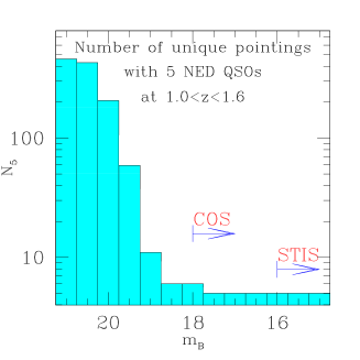
Figure 3.: Left: the number of QSOs with $1.0<z<1.6$ in NED (including the Sloan EDR) as a function of apparent magnitude. Also shown are the rough magnitude limits for high S:N, high resolution spectroscopy with STIS and COS. NED is seriously incomplete at the faintest magnitudes, and the true number density of QSOs rises much more rapidly at faint luminosities than this plot suggests. Right: the number of unique $r=20^{\prime}$ pointings that contain 5 or more of the NED QSOs in the left panel as a function of the imposed QSO magnitude limit. STIS and COS will let us obtain sampling this dense of the HI and metals in the IGM for only a handful of pointing across the entire sky—and the ideal number of QSO in a field this size is much higher than 5. With a somewhat deeper magnitude limit (e.g., $m\sim 20$) dense sampling of the IGM would be vastly easier. The gain is much larger even than this figure suggests because of NED’s incompleteness at fainter magnitudes. See text.

Now let us think how such a survey might be constructed. Obtaining galaxy redshifts in this redshift range is trivial with 8m-class telescopes (e.g., Steidel et al. 1996, Adelberger 2002). That part of the problem is solved. The difficulty lies in obtaining quality spectra of the background QSOs. Over much of the redshift range $1\mathrel{\hbox{\hbox to0.0pt{\hbox{\lower 4.0pt\hbox{$\sim$}}\hss}\hbox{$<$}}}z\mathrel{\hbox{\hbox to0.0pt{\hbox{\lower 4.0pt\hbox{$\sim$}}\hss}\hbox{$<$}}}3$, Lyman-$\alpha$ and (especially) the strongest metal lines lie in the observed near- or far-UV and can only be observed from space. Unfortunately only a small number of QSOs are bright enough to be observed with current and planned space-based UV spectrographs. As an illustration, the left panel of Figure 3 compares the rough high-resolution, high-S:N magnitude limits of STIS and COS to the apparent magnitude distribution of all known QSOs in the (arbitrary) redshift range $1.0<z<1.6$. Only a small fraction of these QSOs are bright enough to observe with either spectrograph. The few hundred sources accessible to COS may seem like more than enough, but this is not true, at least not if the goal (as it should be) is to obtain information about the intergalactic distribution of hydrogen and metals along numerous skewers through the foreground galaxy distribution. This is illustrated by the right panel of Figure 3, which shows, as a function of assumed magnitude limit, the number of unique pointings in the entire sky that contain 5 or more NED QSOs at $1.0<z<1.6$ within a circle of radius $r\sim 20^{\prime}$. The number of QSOs and the circle radius were selected arbitrarily; the plot is designed only to illustrate how much easier it is to find fields with large numbers of background sources as the QSOs’ limiting magnitude becomes fainter. Because NED is increasingly incomplete towards fainter magnitudes, the true gains from a fainter magnitude limit are far larger even than those indicated by this plot.

There are evidently a few known pointings with 5 or more QSOs suitable for COS within a $r=20^{\prime}$ circle. Might these pointings be sufficient for the project we are advocating? The answer, sadly, is no. 5 QSOs per $20^{\prime}$ circle works out to roughly one QSO per $\sim 250$ square arcminutes. For an $\Omega_{M}=0.3$, $\Omega_{\Lambda}=0.7$ cosmology at $z=1.5$, the distance along the plane of the sky between the QSOs in these pointings will typically be more than $10h^{-1}$ comoving Mpc. For comparison, the winds (apparently) detected around galaxies at $z\sim 3$ have a radius smaller than $1h^{-1}$ Mpc. If our goal is to have a few QSOs behind an average galaxy’s expanding blast-wave (in order, e.g., to say something about the blast-wave’s geometry, or learn about the connection between galaxy properties and blast-wave properties on a case-by-case basis), we will need a density of background QSOs that is at least 100 times higher.

A crude estimate of the required spectrographic sensitivity comes from the following calculation, which could and should be improved. Assume the QSO luminosity distribution at the bright end has the shape $n(l)\propto l^{-\alpha}$ with $\alpha\simeq 3.7$ (e.g., Pei 1995). Then the number density of QSOs brighter than magnitude limit $m$ is proportional to $10^{0.4(\alpha-1)m}$, and an improvement in sensitivity of 2 magnitudes over COS would lead to the desired factor of 100 increase in the density of background QSOs.

The good news is that a gain in sensitivity of this size is hardly inconceivable. The required increase in sensitivity over COS+HST is similar to the increase that will come when STIS is replaced by COS, for example. Obtaining the data set that I have described, and settling at last the vexing question of how supernovae have changed the evolution of the baryonic universe, is not much beyond our reach. How long will we have to wait? This is the bad news. The necessary QSO absorption lines are almost all at wavelengths that can only be observed from space; the atmosphere is an obstacle that will not change. Under current NASA plans these data will not be available until most of us are retired or dead.

I would like to acknowledge the major contributions of my collaborators Chuck Steidel, Alice Shapley, and Max Pettini, the support and patience of this meeting’s organizers, and the hospitality of Bukowski’s, in Boston, where much of this polemic was composed.

References

Adelberger, K.L. 2002, PhD Thesis

Adelberger, K.L., Steidel, C.C., Shapley, A.E., & Pettini, M. 2002, ApJ, submitted

Adelberger, K.L. 2003, ApJ, submitted

Cen, R. & Bryan, G. L. 2001, ApJ, 546, 81

Kaiser, N. 1991, ApJ, 383, 104

Pei, Y.C. 1995, ApJ, 438, 623

Pen, U.-L. 1999, ApJ, 510, 1

Ponman, T.J., Cannon, D.B., & Navarro, J.F. 1999, Nature, 397, 135

Springel, V. & Hernquist, L. 2002, MNRAS, in press

Steidel, C.C., Giavalisco, M., Pettini, M., Dickinson, M., & Adelberger, K. L. 1996, ApJ, 462, 17

Weil, M. L., Eke, V. R., & Efstathiou, G. 1998, MNRAS, 300, 773

White, S.D.M. & Rees, M.J. 1978, MNRAS, 183, 341