GALAXIES AND INTERGALACTIC MATTER AT REDSHIFT $Z\sim 3$: OVERVIEW

Abstract

We present the first results from a survey of the relative spatial distributions of galaxies, intergalactic neutral hydrogen, and intergalactic metals at high redshift. We obtained high-resolution spectra of 8 bright QSOs at $3.1<z<4.1$ and spectroscopic redshifts for 431 Lyman-break galaxies (LBGs) at slightly lower redshifts. Comparing the locations of galaxies to the absorption lines in the QSO spectra shows that the intergalactic medium contains less neutral hydrogen than the global average within $r\lower 2.15277pt\hbox{$\;\buildrel<\over{\sim}\;$}0.5h^{-1}$ comoving Mpc of LBGs and more than average at slightly larger distances $1\lower 2.15277pt\hbox{$\;\buildrel<\over{\sim}\;$}r\lower 2.15277pt\hbox{$\;\buildrel<\over{\sim}\;$}5h^{-1}$ comoving Mpc. The intergalactic medium within the largest overdensities at $z\sim 3$, which will presumably evolve into the intracluster medium by $z\sim 0$, is rich in neutral hydrogen and CIV. The lack of HI absorption at small distances from LBGs appears unlikely to be produced solely by the Lyman continuum radiation they emit; it may show that the galaxies’ supernovae-driven winds maintain their measured outflow velocities of $\sim 600{\rm km\,s}^{-1}$ for a few hundred million years and drive away nearby intergalactic gas. We present correlation functions of galaxies with Lyman-$\alpha$ forest flux decrements, with CIV systems, and with other galaxies. We describe the association of galaxies with damped Lyman-$\alpha$ systems and with intergalactic HeII opacity. A strong observed correlation of galaxies with intergalactic metals supports the idea that Lyman-break galaxies’ winds have enriched their surroundings.

1. INTRODUCTION

The large-scale distribution of matter in the universe is well understood only at the earliest times, a few hundred thousand years after the big bang, when primordial photons strained against the opacity of matter and drove small acoustic waves throughout space. But though this era was appealingly simple, elegantly predicted, magnificently observed, and so on, it was nevertheless brief. Particles slowed as the universe cooled. Electrons became unable to outrun the Coulombic pull of nuclei and vanished into atomic orbits. The universe became transparent; the photons of the microwave background hurtled through history; and the baryons left behind, freed from the regulating pressure of light, began to evolve according to their own complicated rules. Many acoustic waves had not even completed their first oscillation when the universe ceased to be described by the simple physics of linear fluid dynamics. Baryons fell towards overdensities in the matter distribution. They crashed together and became shock heated. They cooled. Nuclear reactions ignited. Black holes formed. Intense radiation filled the universe. The final result of this chaos is known only because we can survey the wreckage that surrounds us. A small fraction of baryons were crushed into stars that now huddle together in galaxies, burning through their measure of fuel, dying one by one. Most of the remainder were blasted to $T\sim 10^{5}$–$10^{7}$ K, temperatures they had not experienced since shortly after the big bang, and were left to drift for a sterile eternity in the vast stretches of intergalactic space. Few goals in cosmology are more fundamental than understanding the physical processes that transformed the large-scale distribution of baryons in this way.

Many basic observations suggest that supernovae played a major role. The disruption of star formation by supernova explosions is the favored explanation for why so few baryons are found in stars today (e.g., White & Rees 1978, Springel & Hernquist 2002). Numerical simulations cannot easily reproduce the large disk galaxies that we observe around us (e.g., Weil, Eke, & Efstathiou 1998) or the high temperature of intergalactic gas at redshift $z\sim 3$ (e.g., Cen & Bryan 2001) unless they include substantial heat input from supernovae. The shape of galaxy clusters’ X-ray luminosity/temperature relationship differs from naive self-similar expectations in a way that suggests that supernovae may have imparted $\sim 1$ keV of energy to each of the young universe’s nucleons (Kaiser 1991; Ponman, Cannon, & Navarro 1999). It is difficult to explain why the soft X-ray background is so faint and so dominated by AGN without asserting that supernovae blew apart dense clumps of baryons that would otherwise have produced copious free-free emission (e.g., Pen 1999). The scarcity of faint galaxies in the local universe relative to naive expectations from cold dark matter models is often attributed to the destruction of low-mass galaxies by numerous concurrent supernovae (e.g., Cole et al. 1994).

These examples are only a few among many. We are unable to account for much of what we observe around us without invoking the indistinct notion of strong supernova “feedback,” and our understanding of the evolving universe will remain seriously incomplete until we comprehend quantitatively how this feedback works. Here is what we know: a large fraction of the gas in starburst galaxies at low and high redshift appears to be flowing outwards rapidly enough to escape the galaxies’ gravitational pull (e.g., Heckman et al. 2000; Pettini et al. 2001, 2002); galaxies that experienced intense bursts of star formation in the past now contain little interstellar gas (e.g., Mayall 1958; Roberts 1972); and metals produced by stars can be found far from known galaxies (e.g., de Young 1978; Cowie et al. 1995; Mushotzky & Loewenstein 1997; Ellison et al. 2000). Most attempts to understand how supernovae affect the universe are founded on the picture that these observations inspire: the numerous supernova explosions in a young galaxy create an enormous blast wave that rips through the galaxy and lays waste to its surroundings. But working through the details of this picture remains challenging even after 30 years of theoretical studies (e.g., Mathews & Baker 1971; Larson 1974; Ozernoi & Chernomordik 1978; Ostriker & Cowie 1981; Dekel & Silk 1986; Ikeuchi & Ostriker 1986; Voit 1996; Nath & Trentham 1997; Mac Low & Ferrara 1999; Aguirre et al. 2001; Cen & Bryan 2001; Madau, Ferrara, & Rees 2001; Scannapieco & Broadhurst 2001; Croft et al. 2002). It is still unclear, for example, which sorts of galaxies were responsible for seeding the intergalactic medium with metals, or what effect blast waves have on galaxy formation and evolution, or even whether realistic blast waves would be physically capable of fulfilling the large role that they are assigned in the standard lore.

These blast waves, or “superwinds,” are not easy to study theoretically. Supernovae themselves are not well understood, and treating the propagation of their numerous overlapping shock waves into a galaxy’s inhomogeneous surroundings is difficult enough on its own; but the central problem is that we have little idea of the characteristic energy scale to associate with the winds that supernovae drive. The energy released by a single supernova, $\sim 10^{51}$ erg, is no mystery, but the number of supernovae in a young galaxy is not easy to estimate theoretically or observationally, and it is unclear in any case how large a fraction of the energy released by supernovae is imparted to nascent winds. Much of it may be harmlessly radiated away by the dense gas it heats. Physical arguments and numerical simulations are at present incapable of estimating a priori the energy of a galaxy’s superwind to within even an order of magnitude. Yet the energy of the winds is largely what determines how large an impact they have on the evolving baryonic universe. Current theoretical approaches usually amount to little more than treating the winds’ energy as a free parameter that can be adjusted until supernovae have the desired impact on the rest of the universe—but the circular logic is unsettling to skeptics who wonder if supernovae may be merely a convenient scapegoat for the failures of popular cosmogonic models. The role of supernovae is probably the biggest remaining gap in our attempt to account for the evolution of the baryonic universe since the time of recombination, and this is unlikely to change until observations can provide direct constraints on the strength of supernovae-driven winds.

Inspired in part by these considerations, we began in the spring of 1999 a systematic survey of starburst galaxies and the intergalactic material near them. Our strategy was to apply QSO absorption-line and faint-galaxy techniques to the same volumes of space. Comparing the locations of galaxies and intergalactic absorbing gas would let us map the relative spatial distributions of diffuse and collapsed baryons throughout large volumes of the universe. We felt that these maps would test our understanding of the evolving baryonic universe in a number of ways. Because one of the most robust ways to measure a blast wave’s energy is to see how far out of its galaxy’s potential it has managed to climb, searching for disturbances to the intergalactic gas near galaxies seemed a particularly promising way to measure at last the strength of supernovae-driven winds.

We chose to conduct the survey at redshift $z\sim 3$. Our reasons were primarily practical. First, experience had shown us that galaxies at $z\sim 3$ were easy to find in deep images and easy to study spectroscopically. Second, intergalactic gas at $z\sim 3$ produces a wealth of strong absorption lines that are easily detected from the ground in optical high-resolution spectra of background QSOs. At higher redshifts the galaxy spectroscopy becomes prohibitively difficult (e.g., Steidel et al. 1999) and background QSOs become increasingly rare; at lower redshifts the strongest intergalactic absorption lines can only be detected through difficult space-based spectroscopy. Similar surveys can be constructed at very low redshifts, $z\sim 0$ (e.g., Norman et al. 1996), but it is difficult to cover representative comoving volumes, and in any case simple arguments suggest that the strongest supernova-driven winds likely existed at high redshift, when galaxies were less massive and star-formation rates were far higher (e.g., Adelberger & Steidel 2000, §4).

This paper, the first in a series, describes the survey and its early results. It compares the relative spatial distributions of Lyman-break galaxies (LBGs), intergalactic metals, and intergalactic neutral hydrogen and emphasizes the evidence that star formation in the LBGs directly influences the properties of the nearby IGM. Paper II in the series (Adelberger et al. 2003) sharpens these conclusions, focusing on the unexpectedly strong larger-scale correlations between galaxies and HI in the IGM and the implications for the physics of the IGM. Paper III (Adelberger 2003) examines in more theoretical detail the possibility that superwinds from star-forming galaxies are responsible for the observed correlations between the galaxies and the IGM. We tacitly assume throughout the series that supernovae would be the primary source of any explosive energy release in young galaxies, but AGN are an equally plausible candidate. The source of the energy makes little difference to our conclusions.

§2 presents the observational strategy and some aspects of the data reduction. §3 describes the characteristics of intergalactic gas within $\sim 5h^{-1}$ comoving Mpc of galaxies. This is farther than the galaxies’ winds are likely to propagate, but the discussion sets the stage for §4 where we describe the state of the intergalactic medium nearest the galaxies. It appears to be rarefied and metal-enriched, observations that may suggest the galaxies’ winds have propagated out to comoving radii $r\sim 0.5h^{-1}$ Mpc. In §5 we show the two-dimensional correlation functions of galaxies with galaxies, with intergalactic HI, and with intergalactic CIV. These data show the connection of galaxies and intergalactic gas on spatial scales between those of §3 and §4. §5 contains a brief and largely empirical summary.

2. DATA

2.1. Observations

Our strategy was to use the Lyman-break technique to locate star-forming galaxies at $z\simeq 3.0\pm 0.25$ in fields surrounding background QSOs whose spectra were suitable for measuring Lyman-$\alpha$ absorbing gas at $z\sim 3$. Two criteria were used to select fields. First, we wanted the QSO to lie at $3.3\lower 2.15277pt\hbox{$\;\buildrel<\over{\sim}\;$}z\lower 2.15277pt\hbox{$\;\buildrel<\over{\sim}\;$}3.6$ and to be bright enough for high-resolution spectroscopy. The lower redshift limit was chosen to maximize the number of Lyman-break galaxies at redshifts where HI absorption was probed by absorption in the QSO spectra; the upper limit was chosen to minimize the impact of Lyman-continuum and (especially) Lyman-$\beta$ absorption at higher redshifts upon the $z\sim 3$ Lyman-$\alpha$ forest in each QSO spectrum. Second, we wanted the fields to have as little $100\mu$m cirrus flux from the Galaxy as possible, to minimize the attenuation of Lyman-break galaxies’ light from dust in our own galaxy.

We were able to obtain data in five fields satisfying these criteria (Table 1); one field contains two QSOs. Our sample was augmented to six fields by including data from the “SSA22” region where previous Lyman-break observations (Steidel et al. 1998) had discovered a QSO at $z=3.352$.

Table 1QSO/LBG Fields

QSO	$\alpha_{2000}$	$\delta_{2000}$	$z_{\rm QSO}$	$G_{\rm QSO}$	$R_{\rm spec}$	$t_{\rm spec}$	$\Delta\Omega$	$N_{1}$	$N_{2}$
Primary:
Q0256-0000	02h59m05.6	+00${}^{o}11^{\prime}22^{\prime\prime}$	3.364	18.2	44000	41800	8.5′$\times$ 8.5′	45	38
Q0302-0019	03h04m49.9	-00${}^{o}08^{\prime}13^{\prime\prime}$	3.281	17.8	44000	21000	6.5′$\times$ 6.9′	47	23
Q0933+2845	09h33m37.3	+28${}^{o}45^{\prime}32^{\prime\prime}$	3.428	17.5	33000	28800	8.9′$\times$ 9.3′	65	32
Q1422+2309	14h24m38.1	+22${}^{o}56^{\prime}01^{\prime\prime}$	3.620	16.5	44000	52800	7.3′$\times$ 15.6′	111	62
Q1422+2309b	14h24m40.6	+22${}^{o}55^{\prime}43^{\prime\prime}$	3.629	23.4	6000	43600
SSA22D13	22h17m22.3	+00${}^{o}16^{\prime}41^{\prime\prime}$	3.352	21.6	6000	24600	8.7′$\times$ 17.4′	79	54
Q2233+1341	22h36m27.2	+13${}^{o}57^{\prime}13^{\prime\prime}$	3.210	20.0	44000	68400	9.2′$\times$ 9.3′	47	29
Supplemental:
Q0000-2620	00h03m22.9	-26${}^{o}03^{\prime}17^{\prime\prime}$	4.098	19.4	48000	12500	3.7′$\times$ 5.1′	18	1
Q0201+1120	02h03m46.7	+11${}^{o}34^{\prime}45^{\prime\prime}$	3.610	20.1	44000	40500	8.7′$\times$ 8.7′	19	11

High resolution ($R\sim 40000$; see table 1) spectra of Q0256-0000, Q0302-0019, Q0933+2845, Q1422+2309, and Q2233+1341 were obtained with the HIRES echelle spectrograph (Vogt 1994) on Keck I between 1996 and 2000. Two overlapping echelle grating angles were chosen to provide complete wavelength coverage through the $z\sim 3$ Lyman-$\alpha$ forest. SSA22D13 was observed with the Echellette Spectrograph and Imager (ESI; Sheinis et al. 2000) on Keck II in echellette mode ($R\sim 6000$) in June and August 2000. An ESI spectrum was also obtained for Q1422+2309b, a faint QSO that we discovered $\sim 40^{\prime\prime}$ from Q1422+2309. The HIRES spectra were reduced in the usual way with Tom Barlow’s Makee package. Their continua were fit using an interactive program kindly provided by R. Simcoe. The ESI spectra were reduced and continuum fit with the “Dukee” suite of custom IRAF scripts and C programs written by KLA and M. Hunt.

$U_{n}G{\cal R}$ images were obtained in each field, with COSMIC (Kells et al. 1998) on the Palomar 5m Hale Telescope for Q0256-0000, Q0933+2845, Q2233+1341, and two adjacent pointings in SSA22, and with the Prime Focus Imager on the William Herschel Telescope for Q0302-0019 and Q1422+2309. The Palomar images of Q0933+2845 and WHT images of Q0302-0019 were supplemented with data obtained for another project with MOSAIC on the Kitt Peak 4m Mayall telescope. The images were reduced and photometric catalogs were constructed as described in Steidel et al. (1999). The typical reduced image depths ($1\sigma$) were $\sim$ 29.1, 29.2, 28.6 AB magnitudes per arcsec² in $U_{n}$,$G$, and ${\cal R}$, and approximately 2.2 objects per square arcminute in each field were found to satisfy the Lyman-break selection criteria

$$U_{n}-G\geq G-{\cal R}+1.0,\quad\quad G-{\cal R}\leq 1.2,\quad\quad{\cal R}\leq 25.5.$$ (1)

In Q1422 exceptionally deep data let us extend our sample to ${\cal R}=26$.

Low resolution ($R\sim 600$) spectra for a subset of these Lyman-break candidates were obtained with LRIS (Oke et al. 1995) on the Keck I and II telescopes between 1995 and 2001. Each field was observed through at least 4 multislit masks that accommodated $\sim 20$ objects each. Spectra were obtained for Lyman-break candidates throughout the regions observed in $U_{n}G{\cal R}$, except in the cases of Q0302 and Q0933 where spectra were obtained only in a $\sim 7^{\prime}-9^{\prime}$ region surrounding the QSO rather than throughout the larger imaged fields. The field sizes and number of useful redshifts obtained in each field are listed in Table 1. Figure 1 shows the redshift histogram for our galaxy sample together with the range of redshifts where our QSO spectra could be used to detect intergalactic CIV and HI.

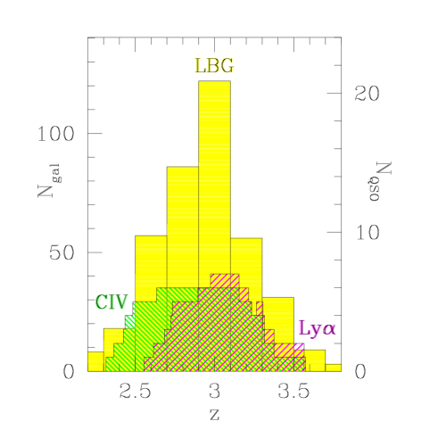
Figure 1.— The range of redshifts probed in our survey. The solid histogram in the background shows the distribution of galaxy redshifts in the primary sample; refer to left axis. The cross-hatched histograms in the foreground show the number of primary-sample QSOs that could be used to detect CIV and Lyman-$\alpha$ at different redshifts; refer to right axis. The Lyman-$\alpha$ histogram conservatively assumes that we could not detect Lyman-$\alpha$ in parts of the spectra that were contaminated by Lyman-$\beta$ from gas at higher redshifts. The CIV histogram assumes that we could not detect CIV in parts of the spectra that were contaminated by Lyman-$\alpha$ from gas at higher redshifts. Neither assumption is strictly true.

These six fields make up the primary sample used in most of our analysis below. In a few cases we also used data in fields surrounding two additional QSOs, Q0000-2620 and Q0201+1120. $U_{n}G{\cal R}$ images for Q0000-2620 were obtained with EMMI on the 3.6m NTT telescope in 1994; images for Q0201+1120 were obtained with COSMIC on the Palomar 5m Hale telescope in 1995. Our echelle spectrum of Q0000-2620 is a combination of a HIRES spectrum taken by W. Sargent and the UVES (Dekker et al. 2000) spectrum made public after the instrument’s commissioning. P. Molaro kindly provided us with the reduced UVES spectrum. A HIRES spectrum of Q0201+1120 was obtained in 1999 and reduced as described above; this spectrum is the same as the one analyzed by Ellison et al. (2001). LRIS on Keck I was used in 1995 and 1996 to measure redshifts for a few objects in each field whose $U_{n}G{\cal R}$ colors satisfied equation 1. We excluded these two fields from most of the analysis for a number of reasons. Their images are shallow. Few spectroscopic redshifts were measured. The $U_{n}G{\cal R}$ filters used for observing Q0000-2620 differed somewhat from those used in the rest of the observations, leading to significant changes in the redshift distribution of spectroscopically observed galaxies. Moreover Q0000-2620 is at so high a redshift that most of the interesting CIV lines are buried in the Lyman-$\alpha$ forest and most of the Lyman-$\alpha$ forest close to our galaxies is badly affected by absorption from Lyman series lines from gas at higher redshifts. The spectrum of Q0201+1120 contains large gaps between echelle orders in the red that prevented us from detecting CIV systems in a uniform way. Nevertheless in two cases below—figures 9 and 10—we were able to make some use of these data.

2.2. Redshifts

2.2.1 Initial wavelength calibration

Of the many steps required to reduce our data, one of the most crucial is the wavelength calibration, the estimate of which wavelengths of light were cast on each pixel by the optics of the spectrograph. This section describes how we calibrated our LRIS data. The HIRES and ESI calibrations were similar.

The data for a single multislit mask typically consisted of three 30 minute exposures followed immediately by a brief spectrum of an arc lamp at the same telescope position as the final exposure. To correct for gravitational flexure of the instrument during the series of exposures, spectra from the earlier exposures were shifted in the wavelength direction as required to make their sky lines overlap with the sky lines in the last exposure. The required shifts often approached but rarely exceeded 3Å($\sim 1$ pixel). The data were then summed and a wavelength was assigned to each pixel based on a 5th order polynomial fit to the wavelength vs. pixel number relationship in the arc-lamp exposure. Occasionally the wavelengths assigned to sky lines by this procedure were systematically incorrect by $\lower 2.15277pt\hbox{$\;\buildrel<\over{\sim}\;$}2$Å; in these cases each spectrum was shifted by a fixed wavelength increment. In the resulting spectra, the mean difference between the true and estimated sky-line wavelengths was negligible and the $1\sigma$ scatter was $\sim 0.25$Å. The wavelengths assigned to each pixel were finally adjusted by small amounts using standard formulae to correct for the motion of the earth around the sun and for the decrease in wavelength due to the index of refraction of air. After applying this procedure (or minor variants) to our data from LRIS, HIRES, and ESI, we were left with spectra in a common vacuum-heliocentric frame that allowed them to be intercompared.

Although this approach is standard, readers should be aware that it is not perfect. For example, assigning correct wavelengths to sky lines in our low-resolution spectra does not guarantee that the wavelength assignment will be correct for the galaxies: if differential atmospheric refraction or errors in slitmask alignment, guiding, or astrometry caused the centroid of a galaxy’s light to be displaced by $0\mbox{${}^{\prime\prime}\mskip-7.6mu.\,$}1$ from the center of its $1\mbox{${}^{\prime\prime}\mskip-7.6mu.\,$}4$ slit, the wavelength solution for the galaxy would differ by $\sim 1$Å from the wavelength solution for the sky lines. We made no attempt to correct for this difficult problem. It may contribute significantly to our derived uncertainties in the galaxy redshifts, which we will shortly discuss.

2.2.2 Correction for galactic winds

The $\sim 30$ km s^-1 velocity of the earth about the sun perturbs our redshifts by $\Delta z\sim 0.0001$. The gravitational flexure of the spectrograph and the slowing of light by the earth’s atmosphere perturb them by larger amounts $\Delta z\sim 0.001$. Larger still are the perturbations due to the chaotic motions of material within Lyman-break galaxies themselves. The various emission and absorption lines within the spectrum of a single Lyman-break galaxy seldom have the same redshift. Absorption lines from the cool interstellar gas tend to have the lowest redshifts; nebular emission lines from the hot gas close to stars tend to have slightly higher redshifts; and Lyman-$\alpha$ almost always has the highest redshift (e.g. Pettini et al. 2002; Pettini et al. 2001). The redshift range spanned by the interstellar lines and Lyman-$\alpha$ often exceeds $\Delta z=0.01$ ($\sim 750{\rm kms}^{-1}$; see Fig. 2). This reflects velocity differences within the galaxy itself—the observed redshift differences are qualitatively consistent with the idea that a typical Lyman-break galaxy is expelling some fraction of its interstellar gas in a supernovae-driven wind (figure 3; see also Tenorio-Tagle et al. 1999)—but if the redshift differences were erroneously assumed to be caused by the Hubble flow, the implied comoving distance between the reddest and bluest features would be $\sim 7h^{-1}$ Mpc ($z=3$, $\Omega_{M}=0.3$, $\Omega_{\Lambda}=0.7$). The challenge is to estimate from our data the redshift of each Lyman-break galaxy’s stars, to pick out where each Lyman-break galaxy lies within the $\sim 7h^{-1}$ Mpc range that our observations would seem to allow.

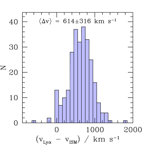
Figure 2.— The distribution of velocity differences between Lyman-$\alpha$ emission and interstellar absorption in the spectra of Lyman-break galaxies.

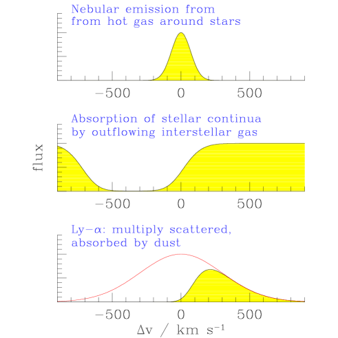
Figure 3.— Schematic view of the different redshifts in the spectrum of a single Lyman-break galaxy. Narrow ($\sigma_{1D}\sim 70$ km s^-1) nebular emission lines have been detected through the near-IR spectroscopy of 27 Lyman-break galaxies. These emission lines presumably lie near the galaxy’s systemic redshift. Wide interstellar absorption lines are usually seen blueward of the nebular lines. Lyman-$\alpha$ emission of varying widths lies redward. The relative redshifts can be understood through a simple wind model for the gas in Lyman-break galaxies. Absorption of stellar continua is produced by outflowing (i.e., blueshifted) gas lying between the observer and the stars. Resonant scattering sends Lyman-$\alpha$ photons on long random walks through the dusty outflow. The few photons that escape without being absorbed by dust are those that were scattered along unusually short paths out of the galaxy; most of these photons scattered off the redshifted back of the outflow and along the steep velocity gradient towards us.

Our approach was guided by the assumption that the redshift of a galaxy’s nebular lines (e.g., [OII]$\lambda 3727$, H$\beta$, [OIII]$\lambda\lambda 4959,5007$) ought to be nearly equal to the redshift of its stars, that the gas responsible for nebular emission should always lie close to hot stars. Because nebular lines are redshifted to the near-IR, where spectroscopy is difficult, we were unable to measure their redshifts for the vast majority of galaxies in our sample. Instead we searched for correlations between nebular-line redshifts and UV spectral characteristics among the 27 Lyman-break galaxies that have measured nebular redshifts, then used these correlations to estimate the systemic redshift of each galaxy in our larger sample from its rest-frame UV spectrum. The near-IR data for 14 of these 27 galaxies were taken from Pettini et al. (2001); our NIRSPEC (McLean et al 1998) spectra of the remaining galaxies will be presented elsewhere.

The following four relationships were found to hold for the 27 galaxies with nebular redshifts. Each resulted from a singular-value decomposition solution of a linear least-squares equation (e.g. Press et al. 1994, §15.4).

Among the galaxies with detectable Lyman-$\alpha$ emission, the velocity of Lyman-$\alpha$ relative to the nebular lines roughly satisfied

$$v_{{\rm Ly}\alpha}\simeq 670-8.9W_{\lambda}\quad{\rm km\,s}^{-1}$$ (2)

where $W_{\lambda}$ is the rest-frame equivalent width of Lyman-$\alpha$ in Å. The rms scatter about this mean relationship was $170{\rm km\,s}^{-1}$. The sense of this correlation is consistent with the idea that dust absorption of resonantly scattered photons is responsible for driving Lyman-$\alpha$ to the red; the reddest Lyman-$\alpha$ lines ought to be the weakest.

Averaging equation 2 over the distribution of $W_{\lambda}$ among galaxies with detectable Lyman-$\alpha$ emission but no detectable absorption lines leads to the mean relationship

$$v_{{\rm Ly}\alpha}\simeq 310\quad{\rm km\,s}^{-1}.$$ (3)

This equation can provide an estimate of a Lyman-$\alpha$–emitting galaxy’s systemic redshift when $W_{\lambda}$ has not been measured, but the redshift’s precision ($\sigma_{v}\sim 250$ km s^-1) suffers. Note that equation 3 is applicable only to data of quality similar to ours, since the adopted distribution of $W_{\lambda}$ was appropriate for galaxies with detectable Lyman-$\alpha$ emission and no detectable interstellar metal lines, and this classification is affected by the signal-to-noise ratio of our typical spectra.

Among galaxies that had both measurable Lyman-$\alpha$ and interstellar-absorption redshifts, the mean of the Lyman-$\alpha$ and interstellar redshifts was larger than the nebular redshift by an amount

$$v_{\rm mid}\simeq-0.014\Delta v-7.0W_{\lambda}+280\quad{\rm km\,s}^{-1}$$ (4)

if $W_{\lambda}$ was used in the fit or

$$v_{\rm mid}\simeq-0.114\Delta v+230\quad{\rm km\,s}^{-1}$$ (5)

if $W_{\lambda}$ was ignored. Here $\Delta v$ is the observed velocity difference between Lyman-$\alpha$ and the absorption lines. The rms scatter about equations 4 and 5 was $150$ and $210{\rm km\,s}^{-1}$ respectively. The physical origins of correlations 4 and 2 are similar.

The mean velocity difference between the interstellar lines and nebular lines for galaxies with measurable interstellar redshifts was

$$v_{\rm abs}\simeq-150\quad{\rm km\,s}^{-1}$$ (6)

with an rms scatter of $160{\rm km\,s}^{-1}$. The qualitative picture of figure 3 suggests that taking account of the velocity widths of the interstellar absorption lines might improve the accuracy of equation 6, but in practice the resolution of galaxy spectra, set by the seeing to $\sim 300$–600 km s^-1 (FWHM), was unusably coarse.

Two anomalous galaxies were excluded when calculating each of these fits and their scatter. The large residuals of the excluded galaxies could be traced back to their unusual spectra. One had two Lyman-$\alpha$ emission lines separated by $\sim 1000$ km s^-1; the other had interstellar absorption at two redshifts separated by more than $1500{\rm km\,s}^{-1}$. As far as we could tell nothing about the UV spectra of these objects would have allowed us to predict their nebular redshifts with much precision. We chose to give up on the 2 pathological cases and optimize our fits for the 25 normal galaxies where we had some chance of success. Readers should be aware that for perhaps 1 galaxy among 10 the equations above will lead to an estimated redshift that is incorrect by several times the quoted rms.

Equations 2 or 3, 4 or 5, and 6 were used to estimate the systemic redshifts of galaxies in our sample that had, respectively, detectable Ly-$\alpha$ emission only, both detectable Ly-$\alpha$ emission and interstellar absorption, and only detectable interstellar absorption. Lyman-$\alpha$ equivalent widths were measured only for galaxies within $60^{\prime\prime}$ of a QSO sightline, because only for these galaxies did the moderately improved precision of equations 2 and 4 relative to 3 and 5 make a significant difference.

We can check the accuracy of our redshift estimates by noting that that the cross-correlation function of galaxies and intergalactic material will be isotropic in an isotropic universe. On average the intergalactic medium ought to be symmetric when reflected in the $z$ direction about the true location of each Lyman-break galaxy. The same is not true for reflection about the measured interstellar or Lyman-$\alpha$ redshift of the galaxies, because these redshifts are influenced only by material that lies between the galaxies’ stars and us, and so the symmetry is broken.

Figure 4 shows the mean Ly-$\alpha$ transmissivity of the intergalactic medium for all pixels of our QSO spectra that lay within an apparent distance of $4h^{-1}$ and $6h^{-1}$ comoving Mpc of a Lyman-break galaxy. Also shown is the mean transmissivity we would have measured had our estimated galaxy redshifts been systematically higher or lower by an amount ranging from $\Delta z=-0.02$ to $\Delta z=+0.02$. The three panels correspond (from top to bottom) to galaxies with only detectable absorption, both detectable absorption and emission, and only detectable emission. In each case the curves of mean transmissivity vs. $\Delta z$ are roughly symmetrical about $\Delta z=0$, which suggests that the systemic redshifts assigned through equations 2, 5, and 6 are accurate on average. The mean redshift offset of the emission and/or absorption lines for each class is marked by the vertical bars. (Readers may find other pertinent data in Figure 25, which is discussed in a different context below).

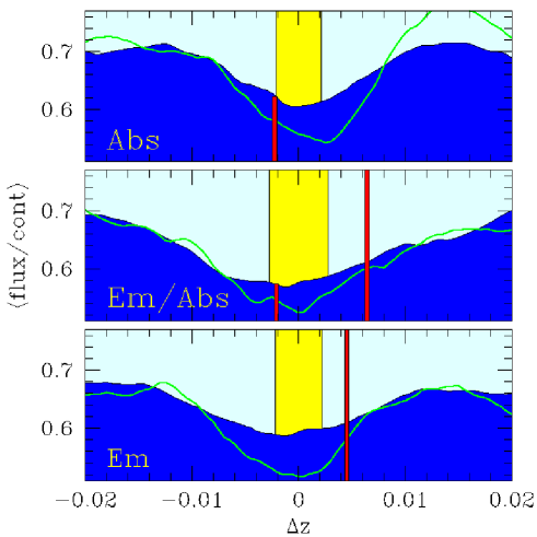
Figure 4.— The mean transmissivity of all parts of the QSO spectra that lie within $4h^{-1}$ (solid line) or $6h^{-1}$ (shaded region) comoving Mpc of a Lyman-break galaxy. The height of these curves at $\Delta z=0$ shows our best estimate from the redshift assignment described in § 2.2.2; the height of the curves at other values of $\Delta z$ shows the mean transmissivity we would have measured had we applied an additional redshift adjustment of $\Delta z$ to each galaxy. Large systematic errors in our redshift estimates would show up as asymmetries about $\Delta z=0$ in this plot, but in fact $\Delta z=0$ lies near the minimum of each curve. The sample was divided into classes defined by the type of features we could detect in each object’s spectrum. The mean redshift of the detected features relative to our assigned redshift is marked with vertical bars, short for absorption lines and tall for emission lines. The size of our estimated uncertainty ($\pm 1\sigma$) in a single galaxy’s redshift is indicated by the rectangular strip surrounding $\Delta z=0$.

Further evidence of the procedure’s accuracy comes from recent work by Shapley et al (2003, in preparation), who used the above equations to shift the spectra of $\sim 800$ LBGs into a common rest-frame. Adding these shifted spectra together revealed weak stellar photospheric lines with velocity $v=0\pm 30{\rm kms}^{-1}$, showing that on average the equations successfully estimate the redshift of the stars in Lyman-break galaxies.

3. GALAXIES AND INTERGALACTIC GAS AT LARGE SEPARATIONS

We are now ready to discuss the relative spatial distributions of galaxies and intergalactic material at $z\sim 3$. This section will concentrate on the properties of the intergalactic gas that lies within a few comoving Mpc of the galaxies in our sample. Simple arguments based on energetics suggest that a wind driven by the supernovae in a Lyman-break galaxy will be unable to propagate more than $\sim 1h^{-1}$ comoving Mpc from its source (e.g., Adelberger 2003), and so data averaged over several Mpc will not tell us much directly relevant to the observed galaxies’ impact on their surroundings. But galaxies ought to form preferentially where the large-scale density of dark matter is high (e.g., Kaiser 1984), and we can expect that the bright galaxies we observe will lie near numerous fainter galaxies and near any sites of previous star formation. The cumulative effect of winds from the seen and unseen galaxies is something the results of this section could in principle reveal.

3.1. HI

One of the most striking aspects of our data is the fact that the transmissivity of the Lyman-$\alpha$ forest tends to be low in volumes that contain a large number of Lyman-break galaxies. Figure 5 shows the Lyman-$\alpha$ forest along skewers through the $\sim 10\times 10\times 10h^{-3}$ comoving Mpc³ cubes that contain the two most significant galaxy overdensities and the two most significant galaxy underdensities in our sample. The mean transmissivity is much lower through the galaxy overdensities. The trend is observed throughout the range of galaxy densities, not merely at the extremes. This can be seen in figure 6, which shows the mean galaxy overdensity in 3-dimensional cells surrounding the QSO sightlines in our primary sample as a function of the mean flux $\bar{f}_{0.02}$ on the $\Delta z=0.02$ sightline segment enclosed by the cell. Each cell was a right rectangular parallelepiped with depth $\Delta z=0.02$ and transverse dimensions equal to its CCD image’s (table 1); in comoving units each was roughly a cube with side-length $13h^{-1}$ comoving Mpc ($\Omega_{M}=0.3$, $\Omega_{\Lambda}=0.7$). The mean galaxy overdensity associated with Lyman-$\alpha$ forest spectral segments with mean transmissivity in the range $\bar{f}_{0.02}\pm\delta\bar{f}$ was calculated by summing the observed number of galaxies in every cell with a mean transmissivity in that range, then dividing by the sum of the number of galaxies that would have been expected in those cells if Lyman-break galaxies were distributed uniformly in space:

$$\langle\delta_{\rm gal}\rangle\equiv\frac{\sum_{i}^{\rm cells}N_{i}}{\sum_{i}^{\rm cells}\mu_{g,i}}-1,$$ (7)

where $N_{i}$ is the observed number of galaxies in the $i$th cell and $\mu_{g,i}$ is the expected number in the absence of clustering. $\mu_{g,i}$ was estimated by scaling our average selection function by the number of galaxies with spectroscopic redshifts in the appropriate field. See appendix B for a justification for this estimator. In order to (slightly) reduce the shot noise, the centers of adjacent cells were separated by $\Delta z=0.004$, so that we oversampled our data by a factor of 5. The QSO spectra were used over the redshift range $(1+z_{q})\lambda_{{\rm Ly}\beta}/\lambda_{{\rm Ly}\alpha}-1<\lambda/\lambda_{{\rm Ly}\alpha}-1<z_{q}-0.05$, where $z_{q}$ is the QSO redshift, in order to avoid contamination of the Lyman-$\alpha$ forest by material associated with the QSO or by Lyman-$\beta$ absorption from gas at higher redshifts. Segments of the QSO spectra with $2.91<\lambda/\lambda_{{\rm Ly}\alpha}-1<2.98$ in SSA22 and with $3.214<\lambda/\lambda_{{\rm Ly}\alpha}-1<3.264$ in Q0933 were removed from the analysis to avoid damped Lyman-$\alpha$ systems.

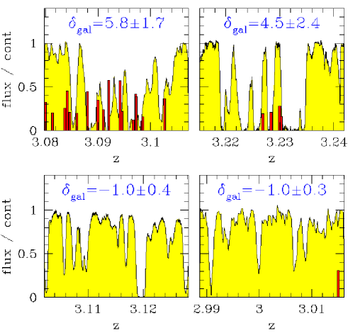
Figure 5.— Intergalactic absorption in the $\sim 10\times 10\times 10h^{-3}$ comoving Mpc³ cells that contain the two most significant galaxy overdensities (top panel) and underdensities (bottom panel). The shaded curves show the Lyman-$\alpha$ forest absorption along segments of our QSO spectra that pass through the overdensities. Each segment is $\sim 17h^{-1}$ comoving Mpc long for $\Omega_{M}=0.3$, $\Omega_{\Lambda}=0.7$. Galaxy redshifts are indicated with vertical lines. The height of each line is proportional to the galaxy’s distance to the QSO sightline; a line reaching ${\rm flux}/{\rm cont}=1$ represents a galaxy $10^{\prime}$ away ($\sim 12.9h^{-1}$ comoving Mpc for $\Omega_{M}=0.3$, $\Omega_{\Lambda}=0.7$). The quoted overdensities $\delta_{\rm gal}$ are measured in a $10h^{-1}$ Mpc cube at the center of the panel. The galaxy overdensity in the upper left panel is the “spike” in SSA22 (e.g., Steidel et al. 1998), the largest galaxy overdensity in the entire Lyman-break galaxy sample and our best candidate for a proto-Abell cluster. These data suggest that the intercluster medium contained a relatively large amount of neutral hydrogen at early times.

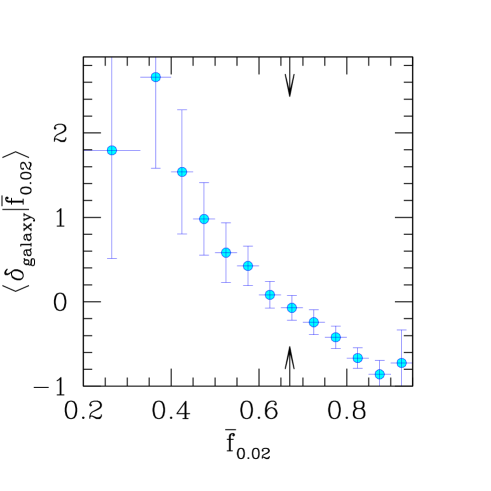
Figure 6.— The mean galaxy density in a $\sim 13h^{-1}$ comoving Mpc cubical cell as a function of the mean Lyman-$\alpha$ forest transmissivity along the $\Delta z=0.02$ sightline skewer through the cell. Galaxy overdensities contain large amounts of neutral hydrogen; galaxy voids contain less. Arrows indicate the mean value of $\bar{f}_{0.02}$ among all sightline segments in our sample.

Some may be surprised that the correlation between HI and galaxy density does not break down at large values of $\langle\delta_{\rm gal}\rangle$. The largest galaxy overdensities in our sample are likely to evolve into rich clusters by $z=0$; this conclusion follows from the comoving volume between $z=2.7$ and $z=3.3$ that we have observed, $\sim 3.7\times 10^{5}h^{-3}$ Mpc³ for $\Omega_{M}=0.3$, $\Omega_{\Lambda}=0.7$, which is large enough to contain $\sim 3$ structures that are destined to evolve into clusters with X-ray temperatures $kT>2.5$keV at $z\sim 0$. We have no better candidates for the protoclusters than the two overdensities shown in figure 5 or (more generally) than the large galaxy overdensities associated with the lowest $\bar{f}_{0.02}$ bins in figure 6. A number of arguments suggest that the intracluster medium was heated at early times, before the cluster itself had formed, and this has led some to speculate that young clusters at $z\sim 3$ might contain far less neutral hydrogen than the universal average (e.g. Theuns, Mo, & Schaye 2001). Figures 5 and 6 show that the opposite is true. The large Lyman-$\alpha$ opacities of (presumed) intracluster media at early times do not imply that preheating has not happened, however, as we will argue in Adelberger (2003): putative shocks traveling outward from high-redshift galaxies and heating the young intracluster medium could easily increase the mean HI content of the volumes they affect. See Adelberger et al. (2003) for an extended discussion of Figure 6 and its implications.

3.2. CIV

The notion that the intergalactic material within galaxy overdensities may have already been preheated receives some support from its observed metal content. The association of Lyman-break galaxies and metals can be quantified in any number of ways, and will receive more attention below; but the qualitative point we wish to make here is adequately illustrated by figure 7. This figure shows the redshifts of the Lyman-break galaxies and CIV systems in the field of Q1422+2309, the QSO with the best spectrum in our sample. The top panel shows the number of galaxies and CIV systems in redshifts bins of width $\Delta z=0.025$. The bottom panel shows the result of smoothing the raw redshifts by a Gaussian with width $\sigma_{z}=0.008$ ($\sim 5.4h^{-1}$ comoving Mpc for $\Omega_{M}=0.3$, $\Omega_{\Lambda}=0.7$) and then dividing by the selection function. The selection function used for the galaxies, shown in the top panel of the figure, is a spline fit to a coarsely binned histogram of every Lyman-break galaxy redshift in our sample. The selection function for CIV systems was approximated as constant with redshift. Though obscured somewhat by shot noise, the connection between galaxy density and CIV density is in fact surprisingly strong; Pearson’s correlation coefficient between the two curves in the bottom panel of figure 7 is 0.61. It is interesting that the amplitudes of the CIV and galaxy fluctuations are comparable. The figure suggests that a volume of the universe which is overdense in galaxies by a factor of $1+\delta\sim 3$ (e.g.) will tend to be overdense in CIV systems by a factor of $\sim 3$ as well. But because Lyman-break galaxies are biased tracers of the matter distribution (e.g., Adelberger et al. 1998), the baryonic overdensity of the same volume will be significantly smaller. This shows that there is more detectable CIV absorption per baryon in galaxy overdensities than elsewhere. One of several possible interpretations is that the intergalactic metallicity is enhanced near galaxies at $z\sim 3$. A similar trend might also result from the density-dependence of carbon’s ionization state.

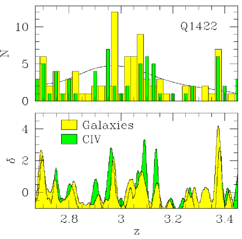
Figure 7.— The redshift distributions of galaxies and CIV absorbers in the field of Q1422+2309. The top panel shows the number of objects observed at each redshift. The bottom panel shows the implied overdensity as a function of redshift after smoothing our raw redshifts by a Gaussian of width $\sigma_{z}=0.008$. The good correspondence of features in the lower panel shows that CIV systems are preferentially found within galaxy overdensities.

3.3. HeII

Heap et al. (2000) obtained a spectrum at wavelengths $1140\lower 2.15277pt\hbox{$\;\buildrel<\over{\sim}\;$}\lambda_{\rm obs}\lower 2.15277pt\hbox{$\;\buildrel<\over{\sim}\;$}1300$Å of one of the QSOs in our sample, Q0302-0019. This spectrum revealed that the HeII Lyman-$\alpha$ ($\lambda_{\rm rest}\simeq 304$Å) optical depth of the intergalactic medium in front of the QSO was large and surprisingly variable. The observed range of optical depths in the spectrum, $\tau_{\rm HeII}\sim 1$ to $\tau_{\rm HeII}\lower 2.15277pt\hbox{$\;\buildrel>\over{\sim}\;$}5$, apparently implies that the hardness of the ionizing background and the ratio of HI to HeII number density must vary significantly in the intergalactic medium at $z\sim 3$. Figure 8 shows that the observed variations in intergalactic HeII opacity appear to be spatially correlated with the locations of galaxies and CIV systems. Excluding the region $z>3.24$, which is presumably affected by radiation from Q0302-0019 itself (e.g. Hogan et al. 1997), and the region $2.987<z<3.016$, which is contaminated by geocoronal Lyman-$\alpha$ emission, we calculate $r_{s}\sim 0.21$, 0.27 for the value of Spearman’s rank correlation coefficient between the smoothly varying galaxy, CIV overdensities shown in figure 8 and the HeII absorption spectrum. The galaxy and CIV overdensities were calculated as described above, near figure 7. Correlation coefficients of this size, $r_{s}\sim 0.2$–$0.3$, do not imply perfect correspondence, and readers will easily find examples in Figure 8 where gaps in HeII opacity have few associated galaxies or metals in our sample (e.g., at $z=2.83$ and $z=3.05$). Nevertheless the statistical correlations visible in the figure are moderately significant. A correlation strength $r_{s}>0.21$ was found for roughly 13% of randomized galaxy catalogs that we correlated with the HeII spectrum; $r_{s}>0.27$ was found for roughly 6% of the randomized CIV catalogs. It is easy to think of reasons that the HeII opacity of the intergalactic medium might decrease near galaxies or CIV systems. The most obvious is that the reionization of HeII should happen first in the dense regions where galaxies, metal-line absorbers, and AGN reside. But this is unlikely to be the full explanation; the HeII optical depth at the mean density at $z\sim 3$ would be of order 1000 if HeII were the dominant ionization state, and so the small but significant fraction of the QSO’s light that is detectable at $\lambda\lower 2.15277pt\hbox{$\;\buildrel<\over{\sim}\;$}1310$Å shows that HeII must already be highly reionized almost everywhere. A more likely explanation may be that the spatial clustering bias of galaxies and AGN causes the number of HeII-ionizing photons per baryon to be largest in overdensities where galaxies and AGN tend to be found. Because the mean free path of 4Ryd photons at $z\sim 3$ is likely to be $\sim 1500$ km s^-1 (Miralda-Escudé, Haehnelt, & Rees 2000), or roughly the size of independent bins in figure 8, we might reasonably expect to see this effect in the figure. We should also add that much of the evidence for a correlation between HeII transmissivity and galaxy or CIV density comes from redshifts $z\lower 2.15277pt\hbox{$\;\buildrel<\over{\sim}\;$}2.9$. If the decrease in HeII opacity at these redshifts reflects a global change in the hardness of the ionizing background due to the growing dominance of AGN (e.g. Songaila 1998; cf. Boksenberg, Sargent, & Rauch 1998), then the correspondence of high HeII transmissivity with the observed galaxy and CIV overdensities would be only a coincidence, and much of our evidence for a connection between galaxies and HeII would be removed.

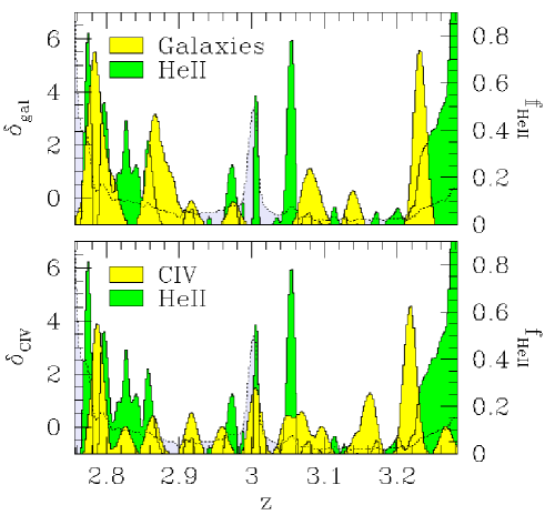
Figure 8.— The correlation between galaxies, CIV systems, and intergalactic HeII transmissivity in the field of Q0302-0019. The curves in the foreground show the overdensity of galaxies and CIV systems as a function of redshift; they were produced by smoothing the list of redshifts with a Gaussian of width $\sigma_{z}=0.008$. The shaded curve in the background shows the HeII Lyman-$\alpha$ absorption seen in the spectrum of Q0302-0019 (Heap et al. 2000) in units of $10^{-16}$ erg s^-1 cm^-2 Å^-1 (refer to right axis). The dotted line is the error spectrum. The HeII content of the IGM is detectably reduced from its mean value in regions where the spectrum significantly exceeds its uncertainty. These regions often (but not always) coincide with galaxy and CIV overdensities.

3.4. Damped Lyman-$\alpha$ systems

For completeness we will briefly describe the association of Lyman-break galaxies with damped Lyman-$\alpha$ systems (table 2). This topic has been recently discussed by Gawiser et al. (2001). Figure 9 compares the mean overdensity of Lyman-break galaxies within cells centered on damped systems to the mean overdensity of Lyman-break galaxies within cells centered on other Lyman-break galaxies. Each cell was a cylinder with height $\Delta z=0.025$ ($\sim 16.7h^{-1}$ comoving Mpc for $\Omega_{M}=0.3$, $\Omega_{\Lambda}=0.7$) and radius equal to value of $\Delta\theta$ shown on the figure’s abscissa. Even at the largest value of $\Delta\theta$ ($265^{\prime\prime}$, or $r\sim 5.7h^{-1}$ Mpc comoving), each cylinder’s diameter is significantly smaller than its height. This helped ensure that galaxies correlated with the central object would fall into the surrounding cell even in the presence of substantial redshift errors. If Lyman-break galaxies and damped systems were similar objects, the mean density of Lyman-break galaxies around damped systems would be similar to the mean density of Lyman-break galaxies around other Lyman-break galaxies, but this is not the case. The observed number of Lyman-break galaxies close to the damped systems in our sample is instead roughly what one would expect if the two populations were independently distributed; we see no evidence for an excess of Lyman-break galaxies near damped systems. In contrast the overdensity of Lyman-break galaxies near other Lyman-break galaxies is large, as the filled circles in figure 9 show. Table 2 compares the observed number of Lyman-break galaxies near each damped system with the number one would have expected if damped systems and Lyman-break galaxies were the same objects. In this case, we would have expected to find 5.96 Lyman-break galaxies within $\Delta\theta=265^{\prime\prime}$, $\Delta z=0.0125$ of the damped systems. Instead we found 2. A Poisson distribution with true mean 5.96 will yield 2 or fewer counts about 6.4% of the time, so the significance of this result is slightly better than 90%. The significance can be assessed in a more empirical way by exploiting the fact that our spectroscopic sampling density in Q0933+2841 and SSA22D13 is very similar to the density in the rest of the Lyman-break galaxy sample. We selected at random from our Lyman-break galaxy catalogs many sets of two galaxies, with one galaxy at roughly the redshift of the damped system in Q0933+2841, the other at roughly the redshift of the damped system in SSA22D13. We then counted the number of other Lyman-break galaxies in cylindrical cells surrounding the two galaxies in each set, and compared to the number of Lyman-break galaxies in cells surrounding the damped systems. The curve in figure 9 shows the frequency $P(>n)$ with which a set of two random galaxies had more galaxy neighbors than the set of two damped systems. The lack of Lyman-break galaxies within $\sim 5.7h^{-1}$ comoving Mpc ($\Delta\theta<265^{\prime\prime}$) of these two damped systems lets us conclude with $\sim 90$% confidence again that bright Lyman-break galaxies and damped systems do not reside in similar parts of the universe. Taken together, the data in figure 9 suggest that the statistical association between damped systems and Lyman-break galaxies is weak; the data are consistent with the idea that damped systems tend to reside in small potential wells that are much more uniformly distributed in space than the massive wells that presumably host Lyman-break galaxies. Others have reached a similar conclusion from different starting points (e.g., Fynbo, Moller, & Warren 1999; Mo, Mao, & White 1999; Haehnelt, Steinmetz, & Rauch 2000).

Table 2Damped Ly-$\alpha$ systems [$+1$]

QSO	$z$	log($N_{HI}/{\rm cm}^{-2}$)	log($N_{CIV}/{\rm cm}^{-2}$)	$N_{\rm obs}$	$N_{\rm exp}$
Q0000-2620	3.3902	21.3	14.7	1	0.67
Q0201+1120	3.3864	21.3	13.9	0	0.45
Q0933+2845	3.2352	20.3	12.8	1	2.23
SSA22D13	2.9408	20.7	13.1	0	2.61
SSA22D13	2.7417	15.1	14.4

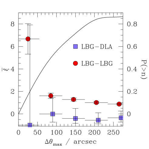
Figure 9.— The spatial association of Lyman-break galaxies and damped Lyman-$\alpha$ systems. Square points show the mean overdensity of Lyman-break galaxies in cylinders of constant depth $\Delta z=0.025$ ($\sim 17h^{-1}$ comoving Mpc for $\Omega_{M}=0.3$, $\Omega_{\Lambda}=0.7$) and variable radius $\Delta\theta$ surrounding the four damped systems in our survey. $250^{\prime\prime}$ corresponds to roughly $5.4h^{-1}$ comoving Mpc in the same cosmology. Circular points show the mean overdensity of Lyman-break galaxies in similar cylinders centered on other Lyman-break galaxies. A $5^{\prime\prime}$ offset was added to the true abscissae of the DLA points. All error bars assume Poisson statistics. Refer to left axis for scale. The curved line shows how frequently randomly chosen Lyman-break galaxies with similar redshifts to the two DLAs in our primary sample have more galaxy neighbors than the DLAs. Refer to right axis. Damped systems do not appear to cluster as strongly as Lyman-break galaxies.

4. GALAXIES AND INTERGALACTIC GAS AT SMALL SEPARATIONS

Any influence of a galaxy’s supernovae on its surroundings should be most pronounced near to the galaxy itself. This makes it especially interesting to study the contents of the intergalactic medium near Lyman-break galaxies. Figure 10 shows the distribution of HI and CIV absorption along the QSO sightline segments that approach Lyman-break galaxies most closely. The angular separation of the galaxy from the sightline is marked in each panel. At $z=3$ one arcminute corresponds to roughly $1.3h^{-1}$ comoving Mpc for $\Omega_{M}=0.3$, $\Omega_{\Lambda}=0.7$, and so at closest approach these sightlines probe the intergalactic medium at $\sim 0.3$ to $1.3h^{-1}$ comoving Mpc from the galaxy. The shaded curves show the Lyman-$\alpha$ forest transmissivity. The symbol $\beta$ appears next to the impact parameter in each panel if Lyman-$\beta$ absorption from gas at higher redshifts could have affected the appearance of the Lyman-$\alpha$ forest at the galaxy’s redshift. The horizontal line marks the mean transmissivity at the galaxy’s redshift, estimated as described in the following paragraph. Circles mark the locations of detectable CIV absorption. The size of each circle is related to the CIV column density; a tripling of a circle’s area corresponds to a factor of ten increase in column density. Due to significant gaps in our echelle spectrum of Q0201, we did not attempt to make a catalog of the CIV systems in this field. Our low quality spectrum of Q1422+2309b did not allow us to detect a significant number of CIV systems; panels for this QSO show the locations of CIV absorption in Q1422+2309 itself, a QSO which is $\sim 1^{\prime}$ away. The short and tall vertical bars mark the observed redshifts of interstellar absorption and Lyman-$\alpha$ emission, respectively, in each galaxy’s spectrum. Wide shaded boxes mark the $1\sigma$ confidence interval on each galaxy’s systemic redshift, estimated from the appropriate equation among 2, 4, and 6.

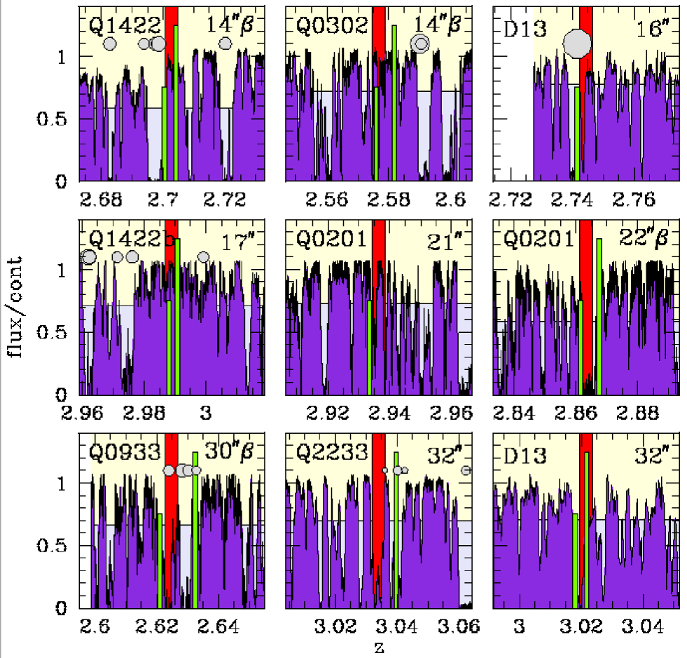
Figure 10.— The distribution of neutral hydrogen and CIV absorption along the segments of the QSO spectra that pass closest to a Lyman-break galaxy. The shaded curve shows the Lyman-$\alpha$ forest. The horizontal line marks the mean transmissivity at this redshift in the QSO’s spectrum. Circles mark the redshifts of detectable CIV absorption. Larger circles correspond to larger CIV column densities; a tripling in the circle’s area corresponds to a factor of 10 increase in column density. Numerical values for the HI and CIV column densities of the absorbing gas near to one of these galaxies can be found in the last entry of table 2. The wide vertical region shows our estimated redshift ($\pm 1\sigma$) for each galaxy. Narrower vertical bars mark the redshifts of Lyman-$\alpha$ (tall bar) or interstellar absorption (short bar) in each galaxy’s spectrum. The distance from each galaxy to the QSO sightline is indicated. $10^{\prime\prime}$ corresponds to roughly $200h^{-1}$ comoving kpc. A $\beta$ next to the distance indicates that the Lyman-$\alpha$ forest at this redshift may be contaminated by Lyman-$\beta$ (or higher) absorption from gas at larger redshifts.

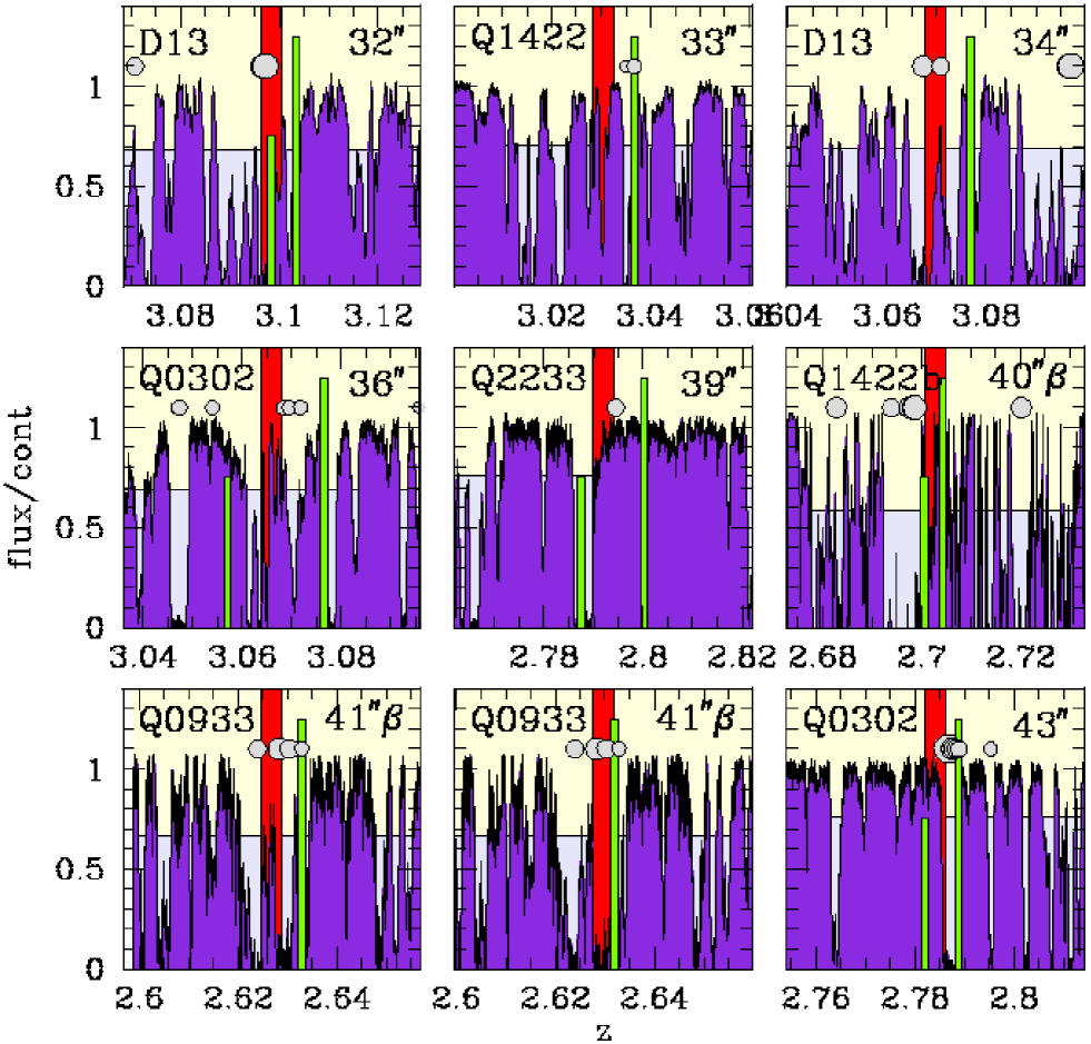
Figure 10.— continued.

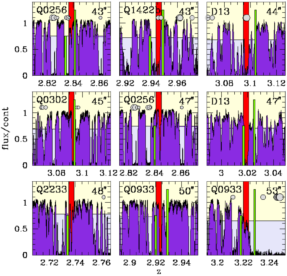
Figure 10.— continued.

The values of the mean intergalactic Lyman-$\alpha$ transmissivity came from the following formulae. When the forest was not contaminated by Lyman-$\beta$ absorption, its mean transmissivity was taken to be

$$\bar{f}(z)=0.676-0.220(z-3),$$ (8)

a fit to the relationship between mean transmissivity $\bar{f}$ and redshift presented by McDonald et al. (2000). The mean transmissivity of the forest contaminated by Lyman-$\beta$ and higher lines is roughly independent of redshift because the increased absorption in the blue due to high Lyman-series lines is largely canceled out by the gradual thinning of the forest towards lower redshifts. The mean transmissivity in this case was found to roughly obey the formula

$$\bar{f}=0.633-0.40(z_{\rm QSO}-3.5)$$ (9)

where $z_{\rm QSO}$ is the QSO’s redshift. These formulae are reasonable approximations only at the redshifts $z\sim 3$ that are of interest to us; they should not be used at other redshifts.

4.1. A lack of HI near Lyman-break galaxies

We would like to draw readers’ attention to an interesting aspect of figure 10. Although the intergalactic medium within $\sim 10h^{-1}$ comoving Mpc of galaxy overdensities appears to contain large amounts of neutral hydrogen (§3.1), often little neutral hydrogen is observed along the small segments of the QSO sightline that pass within $\sim 0.5h^{-1}$ comoving Mpc of a Lyman-break galaxy. This is illustrated more clearly in figure 11, which shows the mean Lyman-$\alpha$ transmissivity of the intergalactic medium as a function of apparent comoving distance from a Lyman-break galaxy. We discarded parts of the QSO spectra that were contaminated by Lyman-$\beta$ absorption from gas at higher redshifts or by damped Lyman-$\alpha$ systems, and normalized the result so that the mean transmissivity at all radii would have been precisely 0.67 if the galaxies in our surveyed volumes were randomly distributed and infinitely numerous. Rough error bars were calculated by generating a large ensemble of fake data sets, each containing the same QSO spectra and same galaxies as our actual sample, but with each galaxy’s redshift modified by a Gaussian deviate with $\sigma_{z}=0.075$ ($\sim 50h^{-1}$ comoving Mpc for $\Omega_{M}=0.3$, $\Omega_{\Lambda}=0.7$). The error bars in the figure show the $1\sigma$ scatter about the mean among these fake data sets. They may be underestimates of the true uncertainty, as discussed below.

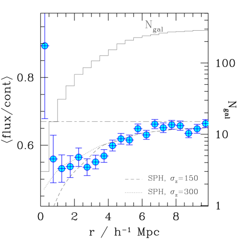
Figure 11.— Mean intergalactic Lyman-$\alpha$ transmissivity as a function of comoving distance from Lyman-break galaxies. Points with error bars mark our measurements; refer to the left axis for the scale. If galaxies were distributed randomly with respect to the Lyman-$\alpha$ forest, we would have measured $\langle{\rm flux/cont}\rangle\simeq 0.67$ at each radius (horizontal line). Instead it appears that Lyman-break galaxies are associated with neutral hydrogen overdensities (i.e., flux decrements) on scales extending to several Mpc, and with HI underdensities on the smallest spatial scales. This behavior, especially on small scales, contrasts with predictions from numerical smoothed-particle hydrodynamic simulations of $\Lambda$CDM universes where galaxies have little impact on surrounding intergalactic matter. In these simulations the mean transmissivity drops increasingly rapidly near galaxies. Examples for different assumed galaxy redshift errors (as labeled, in km s^-1) are shown with curved lines (data from figure 9a of Croft et al. 2002, and scaled arbitrarily in $y$ to match roughly our data on large spatial scales). The number of galaxies in our sample within each radius is shown by the arced staircase (refer to right axis).

Figure 11 shows again the result discussed above (see figures 5 and 6): on scales of $\sim 1$ to $\sim 5h^{-1}$ comoving Mpc Lyman-break galaxies are associated with an excess of neutral hydrogen. But on the smallest scales the trend appears to reverse. Little neutral hydrogen is found within $\sim 0.5h^{-1}$ comoving Mpc of the galaxies. Figure 12 shows that the change in mean transmissivity with distance derives from spatial variations in the relative proportion of lightly and heavily obscured pixels in the Lyman-$\alpha$ forest spectra: few pixels with transmissivities less than 0.5 are found within $\sim 1h^{-1}$ comoving Mpc of a Lyman-break galaxy, while a significant excess of saturated pixels with transmissivity $\sim 0$ are found within $\sim 4h^{-1}$ Mpc of Lyman-break galaxies.

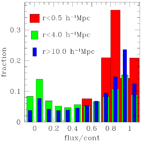
Figure 12.— Histogram of pixel transmissivities at different distances from Lyman-break galaxies. The shape of figure 11 derives from a relative lack of low transmissivity pixels within $r\sim 0.5h^{-1}$ comoving Mpc of Lyman-break galaxies and an excess with $1\lower 2.15277pt\hbox{$\;\buildrel<\over{\sim}\;$}r\lower 2.15277pt\hbox{$\;\buildrel<\over{\sim}\;$}5h^{-1}$ comoving Mpc.

The apparent lack of HI near galaxies is particularly interesting because it seems inconsistent with currently favored numerical models of the intergalactic medium at high redshift. In these models the density of baryons closely traces the density of dark matter and the $\rho^{2}$ dependence of the volumetric recombination rate causes the density of neutral hydrogen to be highest where the density of dark matter is high. But galaxies also form where the density of dark matter is high, and as a result galaxies in the simulations tend to be surrounded by large amounts of neutral hydrogen. In the simplest models the density of HI increases rapidly at small galactocentric radii. This is illustrated by the curved lines in figure 11, which show the mean transmissivity around galaxies with baryonic mass $M_{b}>10h^{-1}M_{\odot}$ in the $\Omega_{M}=0.3$, $\Omega_{\Lambda}=0.7$ smoothed-particle hydrodynamical (SPH) simulation of Croft et al. (2002; taken from their figure 9a).

The differences between the simulation results and our data are not hard to discern. Rather than a continued increase in the HI density at smaller radii, we find that the HI density appears to level off at radii $r\lower 2.15277pt\hbox{$\;\buildrel<\over{\sim}\;$}4h^{-1}$ comoving Mpc and then decrease at the smallest radii $r\lower 2.15277pt\hbox{$\;\buildrel<\over{\sim}\;$}0.5h^{-1}$ Mpc. Although these simulations included many physical processes—gravitational and hydrodynamical interactions, radiative cooling, and radiative heating due to a uniform ionized background—they did not include star formation and supernova feedback in a way that allowed galaxies to have much influence on the nearby intergalactic medium. It is tempting to conclude from figure 11 that the actual impact of galaxies on their surroundings is considerably larger than in the simulations shown. Much of the rest of this section will consider the idea in more detail (see also Croft et al. 2002). But first we would like to discuss the statistical significance of the result.

Our measurement of the mean transmissivity very close to galaxies ($\lower 2.15277pt\hbox{$\;\buildrel<\over{\sim}\;$}1h^{-1}$ comoving Mpc) should be viewed with some skepticism. Recall the large and relatively uncertain offsets that were required to estimate galaxies’ systemic redshifts from the redshifts of the absorption and emission lines in their optical spectra (§ 2.2.2). One need not contemplate figure 10 for long to realize that even minor changes to our estimated systemic redshifts could drastically alter the inferred Lyman-$\alpha$ transmissivity of the intergalactic medium close to Lyman-break galaxies. A few judiciously applied redshift adjustments of $\delta z\sim 0.003$ could easily erase the inflection from figure 11, for example, and $\delta z=0.003$ is hardly a large adjustment. It is small compared to the range of redshifts seen in most Lyman-break galaxy spectra. It barely exceeds our optimistic estimates of the $1\sigma$ redshift uncertainty from § 2.2.2.

One way to assess how badly redshift errors might have compromised our estimate of the mean intergalactic transmissivity at different distances from Lyman-break galaxies is to change each of our redshifts by an amount similar to its uncertainty, then recalculate the implied mean transmissivity. Figure 13 shows the result. Circles mark the average estimated transmissivity at each distance after adding a Gaussian deviate with $\sigma_{z}=0.002$ to each of our redshifts; vertical error bars show the $1\sigma$ range observed when we repeated the exercise many times. Squares show the result when the standard deviation of the Gaussian deviate is increased to $\sigma_{z}=0.004$. Since $\sigma_{z}=0.002$ is roughly the redshift uncertainty that follows from the analysis of § 2.2.2, we conclude that the true redshifts of our galaxies could lie anywhere within our $\sim 2\sigma$ confidence intervals without much affecting our conclusion that the Lyman-$\alpha$ opacity of the intergalactic medium decreases near galaxies.

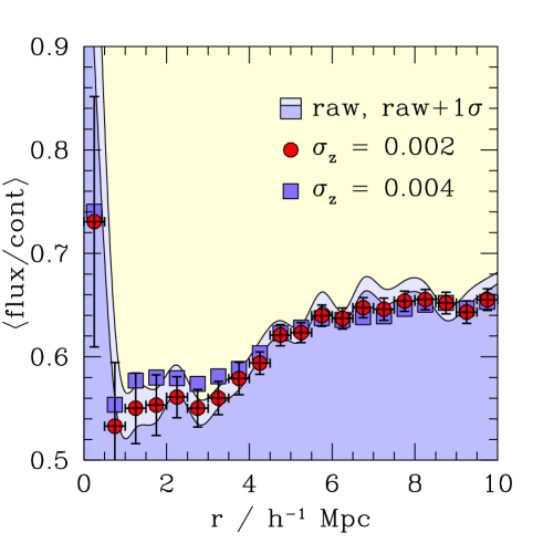
Figure 13.— The result of figure 11 recalculated after modifying each galaxy’s redshift by an amount similar to its uncertainty. Numerous fake data sets were generated by adding to each galaxy’s redshift a Gaussian deviate with the standard deviation $\sigma_{z}$ shown. Points show the average value of the transmissivity among the fake sets; error bars show the $1\sigma$ spread. The error bars for $\sigma_{z}=0.004$, suppressed for clarity, are similar to those for $\sigma_{z}=0.002$. The smooth curves in the background are a spline fit to the data of figure 11 and their $+1\sigma$ upper envelope. If $\sigma_{z}$ were equal to the uncertainty in each galaxy’s redshift, then each of the fake data sets would be roughly as compatible with our observations as the actual data set, and any large differences between the mean transmissivities in the fake and real sets would suggest that the mean transmissivity in the real set may have been compromised by an unusual combination of redshift errors.

The small number of galaxies close to the QSO sight-lines may be more worrying than our redshift uncertainties. Only three galaxies contribute to the measurement of mean transmissivity at $r<0.5h^{-1}$ comoving Mpc that is shown in figure 11. The situation is not quite as dire as the figure suggests, because three additional galaxies in our sample lie within $r=0.5h^{-1}$ comoving Mpc of a QSO sight-line. See figure 10. They were excluded from the calculation shown in figure 11, along with many other galaxies at larger impact parameters, because their low redshifts corresponded to parts of their QSO’s Lyman-$\alpha$ forest that were contaminated by Lyman-$\beta$ absorption and correcting for Lyman-$\beta$ was a challenge that we chose to dodge. But since Lyman-$\beta$ absorption from gas at higher redshifts can only decrease the transmissivity in the Lyman-$\alpha$ forest, there is no reason not to use these galaxies in a conservative search for increases in transmissivity near galaxies. The mean transmissivities within $0.5h^{-1}$ comoving Mpc of the two galaxies in figure 10 at impact parameter $14^{\prime\prime}$ ($\sim 0.28h^{-1}$ Mpc for $\Omega_{M}=0.3$, $\Omega_{\Lambda}$=0.7) are $\langle{\rm flux}/{\rm cont}\rangle=0.92$, $0.97$; the mean transmissivity within $0.5h^{-1}$ comoving Mpc of the galaxy at impact parameter $22^{\prime\prime}$ ($\sim 0.46h^{-1}$ Mpc) is $\langle{\rm flux}/{\rm cont}\rangle=0.04$. Weighting by the length of QSO spectrum that passes within $0.5h^{-1}$ comoving Mpc of each galaxy, this implies a mean transmissivity of 0.78 for the three—an answer encouragingly consistent with the result of figure 11 that was derived from three different galaxies.

Still, six galaxies with impact parameter $r_{\theta}<0.5h^{-1}$ comoving Mpc is not a large sample. The evidence for a decrease in HI density within $0.5h^{-1}$ comoving Mpc of Lyman-break galaxies has a significance of less than $2\sigma$; the difference between our observations and the simulations in the same bin would have a significance of about $2\sigma$ if we pessimistically assumed that the accuracy of our redshifts was only $\sigma_{z}=300{\rm kms}^{-1}$. One might argue that even without the data at $r_{\theta}<0.5h^{-1}$ our measurements would not resemble the simulations perfectly, but it may be more fruitful to consider instead what physical processes could lead to a lack of neutral hydrogen within $\sim 0.5h^{-1}$ comoving Mpc of a galaxy and look for other signatures of their existence.

4.2. Physical origin

4.2.1 Ionizing radiation

Reduced Lyman-$\alpha$ absorption is observed in the intergalactic medium surrounding high-redshift QSOs, a fact that presumably reflects a decrease in the hydrogen neutral fraction in regions where a quasar’s radiation overwhelms the ambient ionizing field (see, e.g., Weymann, Carswell, & Smith 1981; Murdoch et al. 1986; Bajtlik, Duncan, & Ostriker 1988; Scott et al. 2000). Could a similar physical cause account for the lack of HI absorption in the vicinity of Lyman-break galaxies? A rough argument suggests that this is unlikely to be the case. Consider the mean transmissivity within $0.5h^{-1}$ comoving Mpc of an LBG, $\langle{\rm flux}/{\rm cont}\rangle\lower 2.15277pt\hbox{$\;\buildrel>\over{\sim}\;$}0.8$, which is substantially higher than the mean transmissivity $\langle{\rm flux}/{\rm cont}\rangle\sim 0.5$ we might expect in the absence of a proximity effect (Fig. 11). In the $z=3$ output of the SPH simulation described in White, Hernquist, & Springel (2001), an increase in the ionizing background by a factor of $\sim 8$ is required to increase the mean transmissivity of a random section of the Lyman-$\alpha$ forest from 0.5 to 0.8, and so we might guess that the ionizing flux within $0.5h^{-1}$ Mpc of a Lyman-break galaxy would have to be $\sim 8$ times higher than its universal mean if ionizing radiation from the galaxies were responsible for the observed proximity effect. The Lyman-break galaxies in our sample could not easily produce an ionizing flux so large, as the following crude calculation shows. If our sample can be approximated as a uniform population of galaxies with ionizing luminosity $L$ (energy time^-1 frequency^-1) and comoving number density $\rho$ that produces a fraction $f_{\rm bg}$ of the total ionizing background $J_{\nu}^{\rm tot}$ (energy time^-1 frequency^-1 area^-1 steradian^-1) at $z\sim 3$, then the contribution to the ionizing background from a single galaxy at radius $r$ is

$$J_{\nu}^{1}=L/(4\pi r)^{2}$$ (10)

while the net contribution to the ionizing background from the population as a whole is roughly

$$J_{\nu}^{\rm LBG}\sim L\rho(d/c)(c/4\pi)\equiv f_{\rm bg}J_{\nu}^{\rm tot}$$ (11)

where $d$ is the average distance traveled by an ionizing photon before it is absorbed. The ionizing flux will therefore be more than $n$ times higher than its universal average $J_{\nu}^{\rm tot}$ within a radius

$$r_{n}\sim[4\pi\rho(n-1)d/f_{\rm bg}]^{-1/2}$$ (12)

of a Lyman-break galaxy. Assuming an $\Omega_{M}=0.3$, $\Omega_{\Lambda}=0.7$ cosmology, and substituting $d\sim 117h^{-1}{\rm Mpc}$ (i.e., $\Delta z\sim 0.18$) for the comoving effective absorption distance (Madau, Haardt, & Rees 1999) and $\rho\sim 4\times 10^{-3}h^{3}{\rm Mpc}^{-3}$ for the comoving number density of Lyman-break galaxies with magnitude ${\cal R}<25.5$, we find

$$r_{n}\sim\sqrt{f_{\rm bg}/(n-1)}\times 0.4h^{-1}{\rm comoving\,\,Mpc}.$$ (13)

In the extreme case where all of the hydrogen-ionizing background is produced by Lyman-break galaxies with ${\cal R}<27$ (see, e.g., Steidel, Pettini, & Adelberger 2001), only $\sim 50$% of it will be produced by Lyman-break galaxies with ${\cal R}<25.5$, provided that the ratio $f_{\lambda}($1500Å$)/f_{\lambda}($900Å$)$ is independent of luminosity and that the rest-frame 1500Å luminosity distribution of Lyman-break galaxies is a Schechter function with knee ${\cal R}_{*}=24.5$ and faint-end slope $\alpha=-1.6$ (Adelberger & Steidel 2000), and so we can take 0.5 as a rough upper limit on $f_{\rm bg}$. This implies an upper limit of $r_{\rm max}\lower 2.15277pt\hbox{$\;\buildrel<\over{\sim}\;$}0.1h^{-1}$ comoving Mpc for the radius within which ionizing radiation from Lyman-break galaxies could raise the ionizing flux to $\sim 8$ times its universal value and increase the mean transmissivity from 0.5 to 0.8. The argument is crude in a number of ways, but the observed radius with $\langle{\rm flux}/{\rm cont}\rangle\sim 0.8$ is $\sim 5$ times larger than $r_{\rm max}$ and $r_{\rm max}$ does not depend strongly on any of its parameters $f$, $n$, $d$, or $\rho$. The change in mean transmissivity near Lyman-break galaxies appears unlikely to be produced solely by the Lyman-continuum radiation they emit.

4.2.2 Galactic superwinds

Could winds driven by the combined force of numerous supernova explosions within Lyman-break galaxies be responsible instead? Strong winds with velocities exceeding the escape velocity have been observed around a large fraction of starburst galaxies in the local universe (e.g. Heckman et al. 2000). Similar outflows are seen in Lyman-break galaxies as well (§ 2.2.2; Pettini et al. 2001; Pettini et al. 2002). Though the typical velocity of a Lyman-break galaxy’s interstellar lines relative to its nebular lines is only $\sim 150{\rm km\,s}^{-1}$, the velocity exceeds $300{\rm km\,s}^{-1}$ for roughly one third of the galaxies in the sample of § 2.2.2. Moreover the interstellar material within an individual Lyman-break galaxy does not all flow outward at a single rate. Instead a reasonable fraction of the absorbing interstellar material has been accelerated to velocities significantly higher the mean interstellar velocity. Pettini et al. (2002) found absorbing interstellar gas with blueshifts of up to $\sim 750$ km s^-1 in MS1512-cB58, for example, a galaxy with a mean interstellar blueshift of $\sim 250$ km s^-1. The large velocity widths of most Lyman-break galaxies ($\sigma_{v}\sim$ 180–320 km s^-1; Steidel et al. 1996) show that this situation must be common. The typical Lyman-break galaxy apparently contains absorbing material flowing outwards with a range of velocities $0\lower 2.15277pt\hbox{$\;\buildrel<\over{\sim}\;$}v\lower 2.15277pt\hbox{$\;\buildrel<\over{\sim}\;$}600$ km s^-1.

In local galaxies, where similar outflows are observed, a distribution of velocities from 0 to $v_{\rm max}$ is generally interpreted as evidence that winds from supernovae are stripping material from interstellar clouds and accelerating it to the velocity $v_{\rm max}$ (e.g. Heckman et al. 2000). If Lyman-break galaxies’ absorption spectra were interpreted in the same way, one would conclude that most of the absorbing material will eventually be accelerated to a velocity of $\sim 600$ km s^-1. In Adelberger (2003) we consider the implications of 600 km s^-1 outflows from Lyman-break galaxies in some detail. We argue that $\sim 600$ km s^-1 winds should be able to escape potential wells as deep as those that presumably surround Lyman-break galaxies, show that the release of supernova energy implied by the galaxies’ star-formation rates and stellar masses should be sufficient to set massive $\sim 600$ km s^-1 winds in motion, and find that these winds would likely travel a distance comparable the observed radius of the galaxy proximity effect during the typical $\sim 300$Myr star-formation time-scale of Lyman-break galaxies. The upshot is that these winds may plausibly have driven intergalactic material from a cavity of radius $r\sim 0.5$ comoving Mpc surrounding each galaxy, producing the observed lack of neutral hydrogen near the galaxies. In the remainder of this section we will look for other evidence that this might be the case.

4.3. Metals

If Lyman-break galaxies drive winds into their surroundings, one might expect to see an increase in the number density of metal-line absorption systems near them. The discussion above and in Adelberger (2003) suggests that any material ejected by a Lyman-break galaxy would be likely to lie within $\sim 0.5$ comoving Mpc and to have a redshift difference $\lower 2.15277pt\hbox{$\;\buildrel<\over{\sim}\;$}600$ km s^-1. These numbers are uncertain. Aside from the crude spherical model of Adelberger (2003) and its poorly constrained parameters (e.g., the fraction of supernova energy that is imparted to the winds), there are the complications that winds from different galaxies will have advanced to different radii, that winds slow as they advance, and that much of a wind’s velocity may be directed perpendicular to the sightline. Nevertheless the numbers above tell us roughly where we should search for metals that might have been ejected from Lyman-break galaxies.

The QSO absorption spectra available to us clearly cannot provide perfect information about the distribution of metals in the intergalactic medium. In most cases we can detect only the absorption due to CIV, and this is what we will be forced to rely on in the analysis below. Although we will often assume glibly that CIV absorption systems are found where the metallicity is highest, we should remind readers at the outset that the density of CIV is not related in a trivial way to the density of metals: the fraction of carbon that is in the third ionization state can be strongly affected by the local gas density and by the intensity and shape of the ambient radiation field. Still in at least some cases we can be reasonably confident that the presence of CIV absorption near Lyman-break galaxies signals the presence of significantly enriched gas. Our confidence derives from Figure 14, which shows the ratio $\eta\equiv n_{\rm CIV}/n_{\rm HI}$ in ionization equilibrium for a (76% H, 24% He) gas with solar carbon abundance. This ratio depends sensitively on the possible presence of a break at 4Ryd in the background radiation field, since reducing the radiation at $h\nu>4$Ryd makes it harder for CIV to be ionized to CV but does not much affect the density of HI. Nevertheless the plot suggests that most intergalactic gas would likely have $0.1\lower 2.15277pt\hbox{$\;\buildrel<\over{\sim}\;$}\eta\lower 2.15277pt\hbox{$\;\buildrel<\over{\sim}\;$}3$, though the ratio could be driven as high as $\sim 6$ if the temperature and density were carefully chosen and if the intensity of the background radiation decreased sharply at $h\nu>4$Ryd. If the actual abundance of carbon in the gas were $[{\rm C}/{\rm H}]\sim-2.5$, or $\sim$ one $300$th solar, characteristic of the intergalactic medium at $z\sim 3$ (e.g., Davé et al. 1998), one would expect $\eta$ typically to be $\sim 10^{-3}$–$10^{-2}$ and never to exceed $\eta^{\rm max}_{-2.5}\sim 2\times 10^{-2}$. The fact that the observed ratio $n_{\rm CIV}/n_{\rm HI}$ in gas close to Lyman-break galaxies sometimes exceeds $\eta^{\rm max}_{-2.5}$ by an order of magnitude (see, e.g., the entry in table 2 for the $z=2.7417$ system along the SSA22D13 sight-line) shows that the metallicity of this gas must be significantly higher than the mean $[{\rm C}/{\rm H}]\sim-2.5$.

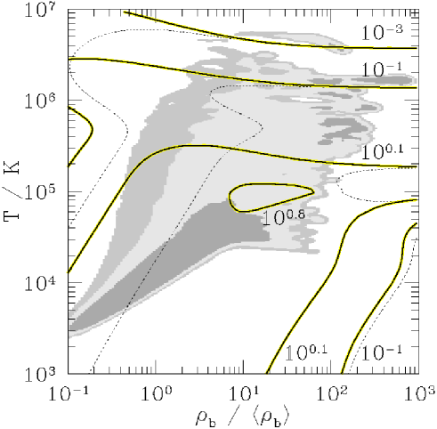
Figure 14.— The ratio $n_{\rm CIV}/n_{\rm HI}$ for a gas with solar carbon abundance in ionization equilibrium with a uniform radiation field. Densities are expressed in terms of $\langle\rho_{b}\rangle$, the mean proper baryon density at $z=3$. Thin dashed lines are appropriate for the background radiation field $J_{\nu}=1.2(h\nu/13.6{\rm eV})^{-1.8}\times 10^{-21}$ erg s^-1 cm^-2 Hz^-1 sr^-1; thick solid lines for the same background except with a factor of 10 reduction for $h\nu>4$ Ryd. The shaded regions show the temperature and density of 68%, 90%, and 95% of the baryonic mass at $z=3$ in the SPH simulation described in White et al. 2001. The upper limit $n_{\rm CIV}/n_{\rm HI}\lower 2.15277pt\hbox{$\;\buildrel<\over{\sim}\;$}6$ for solar carbon abundance shows that gas at the mean intergalactic metallicity $[{\rm C}/{\rm H}]\sim-2.5$ should not have a ratio $n_{\rm CIV}/n_{\rm HI}$ greater than $\sim 0.02$. The measured ratio in gas near to Lyman-break galaxies can exceed this maximum by a large amount, showing that the gas is enriched well beyond the intergalactic mean.

We constructed catalogs of the CIV absorption systems in each QSO’s spectrum by scanning by eye for double absorption lines with the correct spacing and relative strengths for the redshifted CIV$\lambda 1549$ doublet. Rough column densities for each system were estimated with the equation

$$\tau_{\lambda}^{\rm peak}=N_{\rm CIV}\frac{\pi e^{2}}{m_{e}c}f_{\rm CIV}\frac{\lambda_{\rm CIV}}{\sigma_{v}\sqrt{2\pi}},$$ (14)

for the peak optical depth in terms of CIV’s column density $N_{\rm CIV}$, oscillator strength $f_{\rm CIV}$, and (Gaussian) velocity dispersion $\sigma_{v}$, after fitting $e^{-\tau_{\lambda}}$, with $\tau_{\lambda}$ a Gaussian, to both components of the doublet. CIV systems with similar redshifts were treated as independent systems if their velocity differences exceeded twice the quadrature sum of their velocity full widths. In the case of Q1422+2309, our CIV catalog agrees well with the more carefully constructed catalog of Ellison et al. (2000), though it differs somewhat in the arbitrary grouping of neighboring CIV systems into single absorption complexes.

Ten galaxies in our primary sample lie within $\Delta\theta=35^{\prime\prime}$ ($\sim 0.75h^{-1}$ comoving Mpc for $\Omega_{M}=0.3$, $\Omega_{\Lambda}=0.7$) of the QSO sightline. In nine of the ten cases there is detectable CIV absorption in the QSO spectrum within 600 km s^-1 of the galaxy’s redshift. The lone exception lies near the sightline to SSA22D13, a faint QSO whose moderate resolution spectrum reveals only the strongest CIV systems. In three cases, shown in figure 15, the CIV absorption is especially strong and absorption due to many species is evident. The galaxies shown in the figure, SSA22-MD36, Q2233-MD34, and SSA22-C35, lie $17^{\prime\prime}$, $31^{\prime\prime}$, and $33^{\prime\prime}$, respectively, from their background QSO’s sightline; of all the galaxies in our sample, their angular separations to the sightline are the 3rd, 6th, and 8th closest. The metal-line system close to Q2233-MD34 has the largest CIV column density of any in our QSO spectra; the system close to SSA22-MD36 has the third largest. Does this correspondence of metal-line systems with galaxies near the sightline imply some physical connection between the two, or could it be a coincidence? Should we be surprised that 2 of the 3 strongest CIV systems in our sample lie within $\Delta z=600{\rm km\,s}^{-1}$ and $\Delta\theta=35^{\prime\prime}$ of a Lyman-break galaxy?

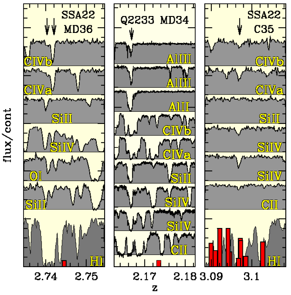
Figure 15.— The Lyman-$\alpha$ and metal absorption along three QSO sightlines than pass within (from left to right) $17^{\prime\prime}$, $31^{\prime\prime}$, and $33^{\prime\prime}$ (90, 180, 170 proper $h^{-1}$ kpc) of known $z\sim 3$ Lyman-break galaxies. Sections of the QSO spectrum corresponding to different species were extracted and aligned. The bottom spectral segment shows the HI absorption; upper segments show the associated metal-line absorption as indicated. Bluer lines are on the bottom. Redshifts with detected metal lines are marked by arrows. Absorption in the extracted spectral segments can be produced by other metal lines at other redshifts, and (in some cases) intergalactic Lyman-$\alpha$ at higher redshift, and the observed absorption can believably be associated with metals at the galaxy’s redshift only when it is observed in more than one line. Galaxy locations are marked with vertical bars, as in Fig. 5; the galaxy closest to the sightline lies in the middle of the extracted spectrum. The velocity offsets between the absorption in the QSO spectrum and the galaxy itself ($\sim 100-600$ km s^-1) are comparable to the measured outflow velocities of the galaxies (e.g. Pettini et al. 2001).

To address this question, we need some estimate of the observed overdensity of Lyman-break galaxies near CIV systems relative to what would be expected if they were distributed independently. We can estimate the number of Lyman-break galaxies that would lie so close to the 3 strongest CIV systems if galaxies and metal systems were independently distributed by generating a large ensemble of fake data sets where each galaxy within $\Delta\theta=35^{\prime\prime}$ of the sightline is assigned a redshift drawn at random from our selection function. See appendix B. Among these fake data sets, the mean number of galaxies that lie within $\Delta z=600{\rm km\,s}^{-1}$ of one of the three strongest CIV systems is $0.049$. Since the observed number is $2$, the implied overdensity of Lyman-break galaxies is $\bar{\xi}_{gc}\sim 40$. Only 1 time in 1000 will sampling from a Poisson distribution with a true mean of $0.049$ yield a value of $\geq 2$, so we can conclude with confidence that strong CIV systems and Lyman-break galaxies are not distributed independently.

But this does not show that the observed metals were driven out of the galaxy by a superwind. The number density of Lyman-break galaxies in cells centered on other Lyman-break galaxies is much higher than the number density in randomly placed cells, for example, yet few believe that one galaxy ejected the next. Is it possible that galaxies and CIV-systems tend to fall near each other for the same reason that galaxies fall near each other, because they all trace the same large-scale structure? A simple way to address this issue is to use the observation of Quashnock & Vanden Berk (1998) that the correlation function of CIV systems at $z\sim 3$ is similar to the correlation function of Lyman-break galaxies, a fact compatible with the idea that CIV systems and Lyman-break galaxies are similar objects. Suppose CIV systems and Lyman-break galaxies were in fact the same objects, but the CIV associated with each galaxy extended only to radii small compared to the smallest galaxy-QSO impact parameter in our sample, so that the detected CIV absorption could never have been produced by a galaxy we observed. In this case we would expect the overdensity of galaxies within $\Delta\theta=35^{\prime\prime}$ and $\Delta z=600{\rm km\,s}^{-1}$ of a CIV system to be roughly equal to the mean overdensity of Lyman-break galaxies within the same distance of another Lyman-break galaxy. Among the 697 Lyman-break galaxies with the most certain redshifts in 13 fields of our survey, 31 unique pairs have a separation $\Delta\theta<35^{\prime\prime}$ and $\Delta z<600{\rm km\,s}^{-1}$ while 3.92 would have been expected if the galaxies were distributed uniformly. The implied galaxy-galaxy overdensity $\bar{\xi}_{gg}=6.9$ is significantly smaller than the measured galaxy-CIV overdensity $\bar{\xi}_{gc}=40$. This suggests the spatial coincidence of Lyman-break galaxies and CIV systems may be too strong to be explained by arguing that both trace the same large scale structure, that both tend to reside in the same clusters and shun the same voids. A more direct connection between the observed CIV systems and galaxies appears to be required.

This sort of argument can be formalized with a statistical inequality derived in appendix A. If $f$ is a discrete (i.e. Poisson) realization of the continuous function $f^{\prime}$, $g$ is a discrete realization of the continuous function $g^{\prime}$, and $\bar{\xi}_{fg}$ denotes the mean value within some volume of the cross-correlation function $\xi_{fg}$ between $f$ and $g$, then $\bar{\xi}_{fg}$ can exceed $(\bar{\xi}_{ff}\bar{\xi}_{gg})^{1/2}$ only if the locations of particles in $g$ are influenced by where particles happen to lie in $f$ or vice versa. This would be the case if (for example) $g^{\prime}$ were equal to $f^{\prime}$ and the particles in $g$ were a random subset of those in $f$, or if each particle in $f$ were surrounded by a cloud of particles in $g$. The statement holds provided the correlation functions are volume averaged with one of a class of 3D weighting functions that includes the Gaussian. If we could show that the Gaussian-weighted cross-correlation function of galaxies and CIV systems $\bar{\xi}_{gc}$ exceeded the root-product of the Gaussian-weighted autocorrelation functions $(\bar{\xi}_{gg}\bar{\xi}_{cc})^{1/2}$, we would have evidence that the number density of galaxies in a random volume directly affected (or was directly affected by) the number density of CIV systems in the same volume.

The mean overdensity of Lyman-break galaxies in Gaussian ellipsoids with $\sigma_{z}=350{\rm km\,s}^{-1}$ and $\sigma_{\theta}=20^{\prime\prime}$ that are centered on the strongest three CIV systems in our sample is $\bar{\xi}_{gc}=21$. The mean overdensity of Lyman-break galaxies in similar ellipsoids centered on other Lyman-break galaxies is $\bar{\xi}_{gg}=7$. The mean overdensity of CIV systems in similar ellipsoids centered on other CIV systems will be comparable, $\bar{\xi}_{cc}\sim 7$, if Quashnock & Vanden Berk’s (1998) estimate of the CIV correlation function remains accurate on small spatial scales. $\bar{\xi}_{gc}$ evidently exceeds $(\bar{\xi}_{gg}\bar{\xi}_{cc})^{1/2}$ by a large amount. This may be an aberration. The sample is small. But if the result holds in a much larger sample of galaxies and CIV systems, we would have solid evidence for a physical link between galaxies and the strong CIV absorption observed $\sim 0.5h^{-1}$ comoving Mpc away.

In any case, the connection between Lyman-break galaxies and CIV systems clearly weakens as the column density of the CIV systems is reduced. If we take the 20 strongest CIV systems, for example, rather than the 3 strongest, the mean overdensity of Lyman-break galaxies in similar Gaussian ellipsoids surrounding the CIV systems is $\bar{\xi}_{gc}=9.0$. This still exceeds $\bar{\xi}_{gg}=7\sim\bar{\xi}_{cc}$, but probably not by a significant amount. The mean overdensity in Gaussian ellipsoids surrounding every CIV system in our sample is a paltry $\bar{\xi}_{gc}=2.8$, showing that there is little evidence that the weakest CIV systems are directly associated with the observed galaxies. The dependence of the cross-correlation strength $\bar{\xi}_{gc}$ on column-density is shown in figure 16. Also shown is $\bar{\xi}_{gg}$ and its uncertainty. Cylindrical cells with $\Delta\theta<35^{\prime\prime}$ and $\Delta z<600{\rm km\,s}^{-1}$ were used when calculating the mean overdensities $\bar{\xi}$, rather than the ellipsoidal Gaussians discussed above. This simplified the calculation of the uncertainties in $\bar{\xi}$, which we optimistically took to be Poisson, but it means that $\bar{\xi}_{gc}$ does not formally need to satisfy inequality A7. But similar conclusions about the column densities where A7 is and is not satisfied would follow had we averaged in Gaussian ellipsoids instead.

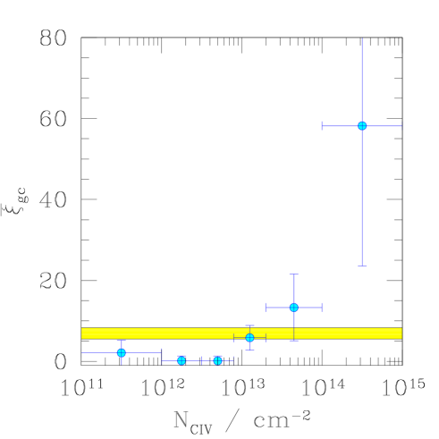
Figure 16.— The observed overdensity of CIV systems within $\Delta z=600$ km s^-1 and $\Delta\theta=35^{\prime\prime}$ of a Lyman-break galaxy as a function of CIV column density. The spatial association of Lyman-break galaxies and CIV systems at these separations grows rapidly stronger as the CIV column density increases. The shaded horizontal region shows the overdensity of Lyman-break galaxies within a similar distance of another Lyman-break galaxy. As explained in § 4.3, the presence of CIV points above this region suggests strong CIV systems and Lyman-break galaxies may be identical objects.

It is interesting to address the association of galaxies and metals in a slightly different way. What fraction of detectable CIV absorption is produced by gas within $\Delta\theta<35^{\prime\prime}$, $\Delta z<600{\rm km\,s}^{-1}$ of a Lyman-break galaxy? Because only a small fraction of the Lyman-break galaxies in any field at $z\sim 3$ are included in our spectroscopic sample, we would not expect most CIV systems to lie near a galaxy in the sample even if every CIV system had a Lyman-break galaxy nearby. Limited observing time allowed us to obtain spectra for fewer than half of the photometrically detected Lyman-break galaxies in each field, for example, and Monte-Carlo simulations (Steidel et al. 1999) suggest that only $\sim 50$% of all Lyman-break galaxies are included in our photometric sample even at $z=3.0$ where our selection is most efficient. We know our sample is seriously incomplete; but we can attempt to correct for this and estimate what fraction of CIV systems would have been found to lie within $\Delta\theta<35^{\prime\prime}$, $\Delta z<600{\rm km\,s}^{-1}$ of a Lyman-break galaxy if we had been able to measure the redshifts of every Lyman-break galaxy our fields. The result is shown in figure 17. Circles mark the fraction $f_{\rm LBG}$ of detected CIV systems with different column densities that lie within $\Delta\theta<35^{\prime\prime}$, $\Delta z<600{\rm km\,s}^{-1}$ of a galaxy in our spectroscopic sample. Stars mark the expected fraction if every CIV system lay within this distance of one (and only one) Lyman-break galaxy. Crosses mark the expected fraction if CIV systems and Lyman-break galaxies were distributed independently. At column densities $N_{\rm CIV}\lower 2.15277pt\hbox{$\;\buildrel>\over{\sim}\;$}10^{13.5}{\rm cm}^{-2}$ the observed number of Lyman-break galaxies close to CIV systems significantly exceeds the number expected if only one Lyman-break galaxy lay within $\Delta\theta<35^{\prime\prime}$, $\Delta z<600{\rm km\,s}^{-1}$ of each CIV system. This apparently shows that the strongest CIV absorption is produced in gas with several Lyman-break galaxies nearby, an interesting observation for which we have no ready explanation. Confidence limits on the fraction of CIV systems that have at least one Lyman-break galaxy within $\Delta\theta<35^{\prime\prime}$ and $\Delta z<600{\rm km\,s}^{-1}$ can be crudely derived by estimating the mean number of Lyman-break galaxies within this distance of a CIV system, $\bar{N}_{\rm LBG}$, then using Poisson statistics to work out how frequently sampling from a distribution with this mean would yield one or more galaxies ($1-e^{-\bar{N}_{\rm LBG}}$). Averaging over the range of $\bar{N}_{\rm LBG}$ compatible with the data leads to the rough confidence intervals shown in figure 17. The data evidently suggest that the majority of CIV absorption with $N_{\rm CIV}\lower 2.15277pt\hbox{$\;\buildrel>\over{\sim}\;$}10^{13}{\rm cm}^{-2}$ is produced by gas that lies no farther than $\Delta\theta<35^{\prime\prime}$ and $\Delta z<600{\rm km\,s}^{-1}$ from a Lyman-break galaxy, i.e., by gas that could plausibly have been ejected from the galaxies in an outflow.

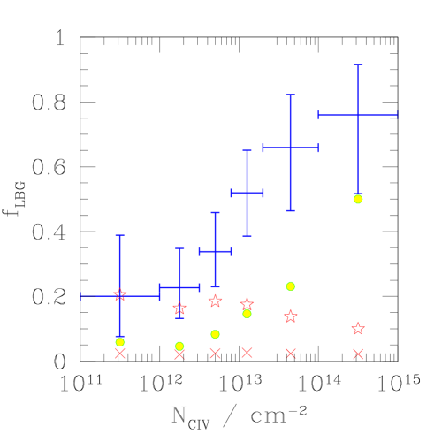
Figure 17.— The fraction $f_{\rm LBG}$ of detected CIV systems that lie within $\Delta z=600$ km s^-1 and $\Delta\theta=35^{\prime\prime}$ of a Lyman-break galaxy as a function of CIV column density. Circles mark the fraction that lie within this distance of a galaxy in our spectroscopic sample. Stars mark the expected fraction if each CIV system had one galaxy within this distance. Crosses mark the expected fraction if CIV systems and Lyman-break galaxies were independently distributed. The low value of $f_{\rm LBG}$ for the stars reflects the severe incompleteness of our spectroscopic sample; simulations suggest that only $\sim$ one fifth of Lyman-break galaxies with redshifts similar to those of the CIV systems would satisfy our photometric selection criteria and be included in our final spectroscopic catalogs. Error bars mark the estimated fraction of CIV systems that lie within $\Delta z=600$ km s^-1 and $\Delta\theta=35^{\prime\prime}$ of a Lyman-break galaxy once our selection effects are corrected.

How might weaker metal-line absorption systems with $N_{\rm CIV}\lower 2.15277pt\hbox{$\;\buildrel<\over{\sim}\;$}10^{13}{\rm cm}^{-2}$ be associated with Lyman-break galaxies? This question can be straightforwardly addressed with results presented in § 5 below. The numerous weak CIV absorbers dominate the cross-correlation function of galaxies and CIV systems, which (as we will show) is roughly a power-law of the form $\xi_{\rm gc}=(r/r_{\rm gc})^{-\gamma_{\rm gc}}$ with $r_{\rm gc}\simeq 3.2h^{-1}$ comoving Mpc and $\gamma_{\rm gc}=1.6$. The mean number of Lyman-break galaxies within a distance $r$ of a randomly chosen CIV system is therefore

$$N_{\rm LBG}\simeq\frac{4}{3}\pi r^{3}n_{\rm LBG}\biggl{(}1+\frac{3r^{-\gamma_{\rm gc}}}{(3-\gamma_{\rm gc})r_{\rm gc}^{-\gamma_{\rm gc}}}\biggr{)},$$ (15)

where $n_{\rm LBG}\simeq 4\times 10^{-3}h^{3}$ Mpc^-3 is the comoving number density of Lyman-break galaxies with magnitude ${\cal R}<25.5$. This shows that the numerous weak CIV systems will typically have $\sim 1$ Lyman-break galaxy within a comoving distance of $\sim 2.4h^{-1}$ Mpc. If they were randomly distributed, the nearest Lyman-break galaxy would lie $\sim 3.9h^{-1}$ Mpc away. Weak CIV systems also tend to lie close to Lyman-break galaxies, though not as close as their higher column-density counterparts.

In summary, it appears that metals in the intergalactic medium are closely connected to the star-forming galaxies we observe. Most CIV systems lie within $\sim 2.4h^{-1}$ Mpc of a Lyman-break galaxy; higher column density systems tend to lie closer still; and the highest column density systems are so strongly correlated with Lyman-break galaxies that we may be forced to conclude that they are the same objects, a result that is remarkable because the absorbing gas is typically $\sim 0.5h^{-1}$ comoving Mpc from the galaxies’ stars.

We are aware of two objections to the implied link between intergalactic metals and Lyman-break galaxies’ winds. The large HI column densities of the metal-line systems significantly exceed naive expectations based on the high expected post-shock temperature of fast-moving winds (Adelberger 2003). The constant observed intergalactic CIV density at redshifts $1.5<z<5.5$ may imply that metal enrichment of the intergalactic medium occurred at $z>5.5$ and not at the lower redshifts we have observed (Songaila 2001). Both objections are reasonable; neither is damning. Cooling due to a plausibly high metallicity in the outflows could account for the large observed HI column densities. Metals ejected by winds might later be driven back into collapsed objects by the continued action of gravitational instability (Adelberger 2003); in this case the constant intergalactic CIV density at $1.5<z<5.5$ would primarily reflect the constant comoving star-formation density (e.g., Steidel et al. 1999) at similar redshifts.

4.4. Interstellar absorption lines

We conclude this section with a brief discussion of the gas that produces the blueshifted absorption lines in the spectra of Lyman-break galaxies. These absorption lines are often called “interstellar,” because they resemble the absorption lines produced by interstellar material in local galaxies. But is it necessarily true that the absorbing material lies between the galaxy’s stars? Or might it instead lie far from the stars, perhaps at the front of a shock that has advanced $\sim 0.5h^{-1}$ comoving Mpc?

It is relatively easy to rule out the idea that the intergalactic CIV absorption observed within $\sim 0.5h^{-1}$ Mpc of Lyman-break galaxies is produced by the same gas responsible for the galaxies’ own absorption lines. The intergalactic equivalent widths are too small. This is illustrated by Figure 18, which compares the mean interstellar CIV absorption in a sample of $\sim 800$ Lyman-break galaxies (Shapley et al. 2003) to the CIV absorption produced by the intergalactic gas that lies $\sim 0.35h^{-1}$ comoving Mpc from the Lyman-break galaxy SSA22-MD36. With a column density $N_{\rm CIV}\simeq 10^{14.4}$ (see table 2), this intergalactic CIV absorption is among the strongest in any of our QSO spectra. But even though its column density is $\sim 2$ orders of magnitude larger than the typical column density in our intergalactic sample, the resulting absorption equivalent width is far smaller than observed in the average Lyman-break galaxy’s spectrum. We have argued that winds from Lyman-break galaxies may reach comoving radii approaching $\sim 0.5h^{-1}$ Mpc, but we cannot claim that most of the outflowing gas responsible for the galaxies’ absorption lines has traveled so far.

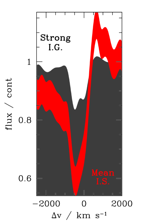
Figure 18.— Intergalactic and interstellar CIV absorption. The thick line in the foreground shows the mean CIV absorption observed in the spectra of Lyman-break galaxies (Shapley et al. 2003, in preparation). The equivalent widths implied by the upper and lower edges of this line differ by $\pm 3\sigma$ from the mean equivalent width reported by Shapley et al. The darker shaded region in the background shows the CIV absorption produced by the intergalactic gas that lies $\sim 0.35h^{-1}$ comoving Mpc from the Lyman-break galaxy SSA22-MD36; it is a small piece of our spectrum of a background QSO that is offset from SSA22-MD36 by $17^{\prime\prime}$. The QSO spectrum was smoothed by a Gaussian with $\sigma=200{\rm kms}^{-1}$ to approximate the resolution of the galaxy spectrum. The intergalactic CIV absorption system is among the strongest in our entire sample, yet its equivalent width is small compared to the CIV equivalent widths observed in the spectra of Lyman-break galaxies themselves. Intergalactic CIV absorption may sometimes be produced by material ejected from Lyman-break galaxies, but not by the same material that produces the galaxies’ own interstellar absorption lines.

The lack of galaxies close to the QSO sightlines prevents us from using the QSO spectra to place tighter limits on the typical distance between Lyman-break galaxies’ stars and interstellar gas. But a comparatively large number of Lyman-break galaxies lie near sightlines towards other Lyman-break galaxies at higher redshift. Since the spectra of the background galaxies are generally good enough to reveal the background galaxies’ own CIV absorption, they should also be good enough to reveal CIV absorption from a foreground Lyman-break galaxy—if the foreground galaxy’s CIV absorption were mainly produced by gas at large impact parameters. 17 Lyman-break galaxies in our complete sample have a background Lyman-break galaxy at an impact parameter of $r_{\theta}<0.16h^{-1}$ comoving Mpc. Among these 17 pairs, the smallest and mean impact parameters are $0.07h^{-1}$ and $0.11h^{-1}$ comoving Mpc respectively. The pairs are generally chance alignments rather than physical associations; all but four have redshifts that differ by more than $\Delta z=0.1$ ($\sim 70h^{-1}$ comoving Mpc for $\Omega_{M}=0.3$, $\Omega_{\Lambda}=0.7$). Figure 19 shows the mean Lyman-$\alpha$ and CIV absorption at the redshift of the foreground galaxy that we observe in the spectra of the 17 background galaxies. In calculating the mean absorption, we discarded parts of the spectra with $\lambda<4000$Å, parts that were contaminated by telluric absorption or by residuals from bright sky lines, and parts that overlapped with any of the background galaxy’s ten strongest absorption lines. Each spectrum was then multiplied by a constant to give it a mean flux of unity within $\pm 5000{\rm kms}^{-1}$ of the foreground galaxy’s absorption line. Little absorption is apparent at the redshifts of the foreground galaxies. We conclude that the typical Lyman-break galaxy’s interstellar absorption lines arise in gas that lies within $\sim 25h^{-1}$ proper kpc of its stars. This conclusion is consistent with the idea that the interstellar absorption is produced by pockets of cold gas entrained in a hot outflow that destroys them before they reach large radii (e.g., Klein, McKee, & Colella 1994 §9.2). It is equally consistent with the idea that Lyman-break galaxies’ winds rarely propagate so far.

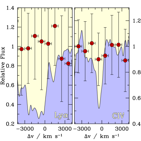
Figure 19.— Similar to Figure 18, except this plot compares Lyman-break galaxies’ strong observed interstellar Ly-$\alpha$ and CIV absorption (curves shaded beneath) to the undetected absorption that foreground Lyman-break galaxies produce in the spectra of background Lyman-break galaxies at small impact parameters $20<r_{\theta}<40h^{-1}$ proper kpc (points). Seventeen galaxy pairs have impact parameters so small. The points’ vertical error bars show the rms dispersion in relative flux at each velocity offset among many sets of 17 galaxy pairs drawn at random (with duplication allowed) from the 17 galaxy pairs with $20<r_{\theta}<40h^{-1}$ proper kpc.

5. CORRELATION FUNCTIONS

The previous sections were primarily concerned with spatial averages over the auto- and cross-correlation functions of galaxies, CIV systems, and Lyman-$\alpha$ forest flux decrements. These averages highlighted the aspects of the spatial association of galaxies, metals, and gas that we found most interesting. But readers may wonder how our conclusions would alter if we averaged the correlation functions over different volumes, or may wish to know how galaxies and intergalactic material are associated on spatial scales other than those we considered. This section presents the correlation functions with no spatial averaging imposed.

5.1. Two dimensional

Figures 20 and 21 show the two dimensional correlation functions of galaxies with galaxies, of galaxies with detected CIV systems, and of galaxies with Lyman-$\alpha$ forest flux decrements. The data used to generate the two figures were identical; figure 21 is less heavily smoothed to help bring out the behavior of the correlation functions on small spatial scales. The abscissae correspond to angular separations $r_{\theta}$ on the plane of the sky; the ordinates correspond to redshift separations $r_{z}$. Observed separations in arc-seconds and in redshift were converted to the comoving distances implied for an $\Omega_{M}=0.3$, $\Omega_{\Lambda}=0.7$ cosmology. The value of the correlation function $\xi_{gc}$ between galaxies and CIV systems at separation $r_{\theta}$, $r_{z}$ was estimated with the statistic

$$\hat{\xi}_{gc}=(D_{g}D_{c}-D_{g}R_{c}-R_{g}D_{c}+R_{g}R_{c})/R_{g}R_{c}$$ (16)

(e.g. Landy & Szalay 1993) where $D_{g}D_{c}$ is the observed number of galaxy–CIV-system pairs with separation $r_{\theta},r_{z}$, $D_{g}R_{c}$ is the number of pairs with the same separation between our galaxy catalog and a random catalog of CIV systems, and $R_{g}R_{c}$ is the number of pairs with the same separation between a random galaxy catalog and random CIV catalog. The correlation functions $\xi_{gf}$ of galaxies with Lyman-$\alpha$ flux decrements and $\xi_{gg}$ of galaxies with galaxies were estimated similarly. The random galaxy catalogs were generated by assigning each galaxy in the true catalog 1000 redshifts drawn at random from our selection function; the angular positions of galaxies in the random and real catalogs were the same. The random CIV catalogs were generated by assigning each CIV system in the true catalog 1000 redshifts drawn from a uniform distribution between the minimum and maximum redshifts where our QSO spectra allowed us to detect CIV systems; the observed number density of detected CIV systems among our QSO spectra at each redshift is closely approximated by a constant once the different redshift selection ranges are taken into account. The random flux decrement spectra were linear functions with the form of equation 8, but scaled to match the observed mean transmissivity of each QSO spectrum. The galaxy-galaxy correlation function was calculated using only data in the redshift range $2.6<z<3.4$, to minimize the effect on our result of the poorly determined wings of the selection function. The calculation of the galaxy-flux cross-correlation function excluded data with $z<2.6$, with $z>3.4$, with $z>z_{\rm QSO}-0.05$, and with $z<(1+z_{\rm QSO})\times 1026/1216-1$. The final criterion excludes portions of the Lyman-$\alpha$ forest that are contaminated by Lyman-$\beta$ absorption from material at higher redshifts. Also excluded were data at the DLA-contaminated redshifts $2.91<z<2.98$ in SSA22 and $3.214<z<3.264$ in Q0933+2841. The galaxy-CIV cross-correlation function calculation excluded data with $z<2.6$, $z>3.4$, $z>z_{\rm QSO}-0.05$, or $z<(1+z_{\rm QSO})\times 1216/1549-0.99$. The last two criteria exclude CIV lines that lie close to the QSO redshift or in the Lyman-$\alpha$ forest. To help guide the eye, the resulting raw two-dimensional correlation functions were finally smoothed by two-dimensional Gaussians with $\sigma_{\theta}=\sigma_{z}=0.5h^{-1}$ (figure 20) or $\sigma_{\theta}=\sigma_{z}=0.2h^{-1}$ (figure 21) Mpc comoving.

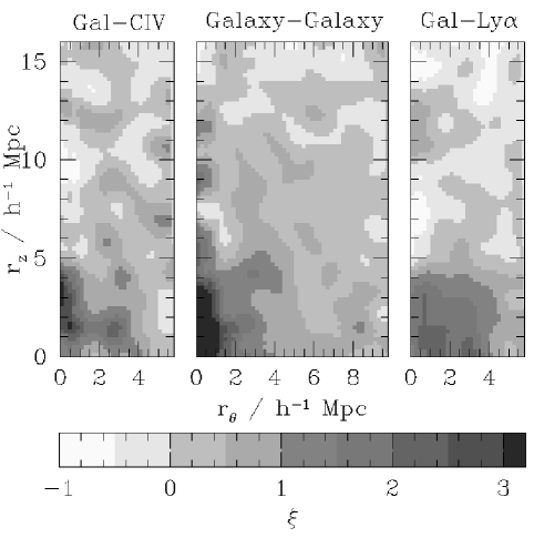
Figure 20.— The two dimensional auto- and cross-correlation functions of galaxies with galaxies, with CIV systems, and with intergalactic Lyman-$\alpha$ transmissivity. The galaxy–transmissivity correlation function is multiplied by $-10$. Each correlation function was smoothed by a two-dimensional Gaussian with $\sigma=0.5h^{-1}$ comoving Mpc.

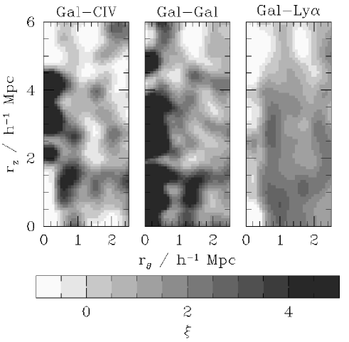
Figure 21.— The correlation functions of figure 20 less heavily smoothed ($\sigma=0.2h^{-1}$ comoving Mpc).

Aside from some elongation in the redshift direction at small separations, which is at least partly due to errors in galaxy redshifts, these two-dimensional correlation functions are reasonably isotropic. This can be seen in figure 22. The figure shows the average value of each correlation function $\bar{\xi}$ in three-dimensional ellipses of comoving volume $4\pi(4h^{-1}{\rm Mpc})^{3}/3$ as a function of axial ratio $r_{z}/r_{\theta}$. The galaxy-galaxy correlation function is the most elongated in the redshift direction, reaching a maximum of $\bar{\xi}$ at $r_{z}/r_{\theta}\sim 1$–$1.6$. This is presumably because galaxy redshift errors have twice the impact and because close galaxy pairs tend reside in dense parts of the universe where the pair-wise velocity dispersion is highest. But the two averaged cross-correlation functions both hit an extremum at $r_{z}/r_{\theta}=1.0\pm 0.2$, demonstrating their isotropy on $\sim 4h^{-1}$ Mpc scales. If one were convinced that the cross-correlation functions should be isotropic despite possible peculiar velocity distortions and despite the significant errors in our galaxy redshifts, figure 22 would show that the Alcock-Paczynski (1979) test at $z\sim 3$ favors a $\Lambda$ cosmology; if we had assumed $\Omega_{M}=1.0$, $\Omega_{\Lambda}=0$ or $\Omega_{M}=0.3$, $\Omega_{\Lambda}=0$ instead of $\Omega_{M}=0.3$, $\Omega_{\Lambda}=0.7$, we would have found that the averages hit their extrema at $r_{z}/r_{\theta}\sim 0.8$ not $r_{z}/r_{\theta}\sim 1.0$. In any case, one unsurprising implication of the lack of redshift elongation in the cross-correlation functions is that the bulk of intergalactic absorbing material is not flowing outwards with respect to nearby galaxies; the peculiar velocities of intergalactic material relative to galaxies is not sufficient to make the galaxy–intergalactic material cross-correlation functions be significantly more elongated than the galaxy–galaxy correlation function. There is no contradiction with the galactic superwind hypothesis because a wind’s evolution is dominated by its stalling phase and because in any case only a small fraction of the intergalactic volume would be affected by active winds at any time (e.g., Adelberger 2003).

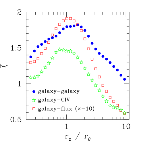
Figure 22.— Average value $\bar{\xi}$ of the auto- and cross-correlation functions of figures 20 and 21 within ellipses of volume $4\pi(4h^{-1})^{3}/3$ comoving Mpc³ as a function of the axial ratio $r_{z}/r_{\theta}$. $\bar{\xi}$ reaches an extremum close to $r_{z}/r_{\theta}=1$ for each correlation function, showing that they are reasonably isotropic on these scales.

The scale dependence of correlation functions is often easiest to apprehend when they are presented as one-dimensional rather than two-dimensional functions. It would be trivial to average the correlation functions of figure 20 in circular annuli, but because of peculiar velocities and redshift measurement errors, a more robust estimate of the one-dimensional correlation functions will come from another approach.

5.2. One dimensional

Appendix C describes the approach adopted by Adelberger (2000) to estimate the one-dimensional auto-correlation function of Lyman-break galaxies at $z\sim 3$. Following Davis & Peebles (1983), we first estimated the projected correlation function, which is a marginalization in the redshift direction of the two dimensional correlation function (e.g., a marginalization of figure 20 or 21). We then estimated the shape of the one-dimensional correlation function from a power-law fit to the projected correlation function. See appendix C. An identical approach can be used to estimate the cross-correlation function of galaxies with CIV systems. Figures 23 and 24 show the auto-correlation function of the $\sim 700$ galaxies with the most secure redshifts in the Lyman-break sample of Steidel et al. (2003; in preparation) and the cross-correlation function of galaxies and CIV systems in the sample of this paper. In both cases the data appear to be reasonably well fit by a power-law of the form $\xi(r)=(r/r0)^{-\gamma}$, justifying the method we have adopted. The best-fit values and $1\sigma$ uncertainties of $\gamma$ and $r_{0}$ are shown in the figures.

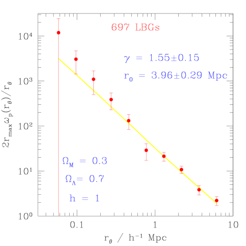
Figure 23.— The projected correlation function of Lyman-break galaxies. The parameters of the best power-law fit to the three-dimensional correlation function $\xi(r)=(r/r_{0})^{\gamma}$ are shown.

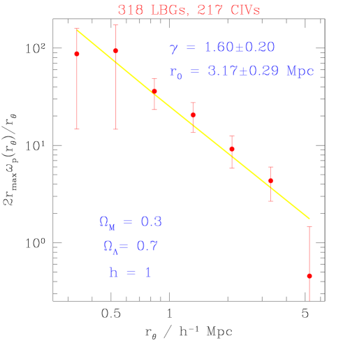
Figure 24.— The projected cross-correlation function of CIV systems and Lyman-break galaxies.

The galaxy-CIV cross-correlation function resembles the galaxy-galaxy correlation function to a large extent. The slopes are identical; the correlation lengths differ by only $\sim 20$%. This suggests that galaxies and CIV systems may be similar objects, a point that has been made by Sargent, Steidel, & Boksenberg (1988), by Quashnock & Vanden Berk (1998), and by us (§ 4.3 above) on slightly different grounds.

Unfortunately we were unable to estimate the cross-correlation function between galaxies and Lyman-$\alpha$ transmissivity with a similar approach. The difficulty is that (after the first $\sim$ Mpc) the HI content of the IGM appears to decline quite slowly with increasing distance from a galaxy. This can be guessed from figure 11, but is seen most robustly in figure 25, which shows cuts along the redshift direction through the two-dimensional galaxy-transmissivity cross-correlation function. To improve the statistics, data for $r_{\theta}<1.1h^{-1}$ Mpc were estimated from the absorption that foreground LBGs produce in the spectra of background LBGs (see § 4.4 for more details); at larger separations the data are the same as in figure 20. One must advance to a impact parameter $r_{\theta}\lower 2.15277pt\hbox{$\;\buildrel>\over{\sim}\;$}4h^{-1}$ comoving Mpc before the net Lyman-$\alpha$ absorption within velocity separations $-600<\Delta v<600{\rm kms}^{-1}$ decreases to half its value at the smallest impact parameters $r_{\theta}\lower 2.15277pt\hbox{$\;\buildrel<\over{\sim}\;$}1h^{-1}$ Mpc. This implies that the slope $\gamma_{\rm gf}$ of the galaxy/transmissivity correlation function lies precariously close to the values $\gamma_{\rm gf}\leq 1$ that cause our statistical deprojection (equation C14) to break down entirely. Although the best formal fit of a power-law correlation function to the data in Figure 25 (marginalized by $\pm 6h^{-1}$ comoving Mpc, or $\sim\pm 670{\rm kms}^{-1}$) has $r_{0}\sim 0.49h^{-1}$ comoving Mpc, $\gamma\sim 1.15$, the data are almost equally compatible with $\gamma_{\rm gf}\leq 1$, and that complicates our attempts to place confidence intervals on the parameters. In any case the best fit parameters depend uncomfortably on the distance over which we marginalize the data. The problem is that the measured mean transmissivity stays slightly lower than the global mean even at large distances from galaxies (cf. figure 11), and it is unclear whether this is part of the true correlation function or merely a $\sim$ percent level systematic error due (e.g.) to our continuum fitting. Fitting the two-dimensional data directly with a power-law smoothed by a Gaussian in the redshift direction does not help. None of our fits filled us with complete confidence. We shall defer a proper estimate of the galaxy-transmissivity correlation function.

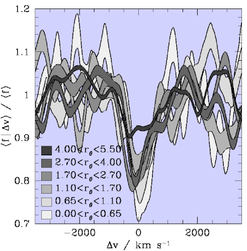
Figure 25.— Cross-cuts through the galaxy-transmissivity cross-correlation function (plus one) at different angular separations (as marked, in $h^{-1}$ comoving Mpc). The line for $4<r_{\theta}<5.5h^{-1}$ Mpc (for example) shows how the typical Lyman-$\alpha$ transmissivity of the intergalactic medium varies along a line that passes a Lyman-break galaxy at an impact parameter of $\sim 4$–$5$ Mpc. The transmissivity is near the global mean $\langle f\rangle$ at large redshift separations from the galaxy, begins to fall within $\sim 1000{\rm kms}^{-1}$ of the galaxy, and reaches a minimum near the galaxy’s redshift. Data for $r<0.65h^{-1}$ Mpc were calculated from the absorption that foreground LBGs produce in the spectra of background LBGs; the galaxy proximity effect should not be detected in this data because the resolution of our galaxy spectra ($\sim 500{\rm kms}^{-1}$ FWHM, or $\sim 4.5h^{-1}$ comoving Mpc) significantly exceeds the $\lower 2.15277pt\hbox{$\;\buildrel<\over{\sim}\;$}1h^{-1}$ comoving Mpc diameter of the region around each galaxy that appears to have a lowered HI content.

The uncertainty in the shape of the galaxy-flux correlation function does not stop us from making one final observation: the ratio of CIV to HI in the intergalactic medium almost certainly increases as one approaches a Lyman-break galaxy. The mean Lyman-$\alpha$ transmissivity of the intergalactic medium does not change much with distance from a Lyman-break galaxy, only by $\lower 2.15277pt\hbox{$\;\buildrel<\over{\sim}\;$}30$% (cf. figure 11), so it may be a reasonable first approximation to assume that the density of intergalactic HI is roughly independent of distance to a Lyman-break galaxy. But the number density of CIV systems depends very strongly on distance to a Lyman-break galaxy; according to the power-law fit described above, the density of CIV systems is $\sim 6.4$ times higher at $r=1h^{-1}$ comoving Mpc than at $r=10h^{-1}$ Mpc. Readers may wish to refer to Figure 26, which shows marginalizations by $\pm 6h^{-1}$ comoving Mpc in the redshift direction over the two-dimensional correlation functions of Figure 20. The marginalization reduces the differences between the correlation functions somewhat, but nevertheless they are clear. The significantly different strengths of the galaxy-CIV and galaxy-transmissivity correlation functions make it seem almost inevitable that the ratio of intergalactic CIV to HI density increases dramatically close to Lyman-break galaxies—though we should emphasize again that neither the mean Lyman-$\alpha$ transmissivity nor the number density of CIV systems is related in a simple way to column density. One may demonstrate through simple calculations, omitted at the referee’s request, that increasing the intensity of the radiation field at $z\sim 3$ would lead to a decrease in the CIV content of most of the Lyman-$\alpha$ forest. This shows that radiation from Lyman-break galaxies is unlikely to account for any enhancement in CIV density near to them. Figure 14 shows that plausible changes in the intergalactic density and temperature near the galaxies would be unlikely to change $n_{\rm CIV}/n_{\rm HI}$ by a factor of $\sim 6$. We conclude that the simplest explanation for the (apparently) strong change of $n_{\rm CIV}/n_{\rm HI}$ with radius may be that the intergalactic metallicity is higher near the galaxies. See Steidel et al. (2003; in preparation) for a less superficial analysis.

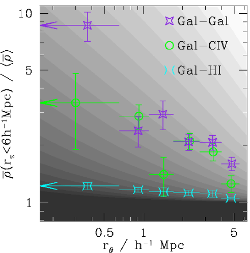
Figure 26.— Marginalizations over $0<r_{z}<6h^{-1}$ comoving Mpc of the data shown in figure 20. Points with error bars show the marginalized galaxy-galaxy, galaxy-CIV system, and galaxy/Ly-$\alpha$ transmissivity correlation functions plus one. The plot shows (for example) that a cylinder of depth $r_{z}=\pm 6h^{-1}$ Mpc and radius $r_{\theta}=0.65h^{-1}$ Mpc centered on a typical LBG will contain $\sim 9$ times the number of (other) LBGs and $\sim 3.5$ times the number of CIV systems as a similar cylinder randomly placed. Other bins of $r_{\theta}$ on the plot correspond to volumes that are cylindrical annuli centered on LBGs rather than cylinders. To improve the statistics, the galaxy-HI measurement at the smallest separation was estimated from the absorption that foreground LBGs produce in the spectra of background LBGs; see § 4.4. Striations in the background show how this plot would appear if the unmarginalized density had the form $\rho(r)\propto 1+(r/r_{0})^{-1.6}$.

6. SUMMARY

The goal of this paper was to compare the spatial distributions of galaxies, metals, and neutral hydrogen at high redshift. We conducted a redshift survey of $z\sim 3$ Lyman-break galaxies in 6 primary fields containing QSOs at $3.1\lower 2.15277pt\hbox{$\;\buildrel<\over{\sim}\;$}z\lower 2.15277pt\hbox{$\;\buildrel<\over{\sim}\;$}3.6$ whose spectra revealed the locations of HI and metals along sightlines through the galaxy distributions. We quantified the relationship between galaxies and intergalactic material by calculating two-point correlation functions or closely related statistics. Various averages over the correlation functions were presented in §§ 3 and 4; the one-dimensional and two-dimensional correlation functions of galaxies with galaxies, with CIV systems, and with Lyman-$\alpha$ forest transmissivity were presented in § 5. The most lasting contribution of this paper may be its methodology, which will be applied to a larger sample in the future. Applying these statistical methods to the present sample leads to the following principal conclusions:

1. The HI content of the intergalactic medium is closely correlated with the positions of nearby galaxies. The material within $r\sim 0.5h^{-1}$ comoving Mpc of Lyman-break galaxies absorbs Lyman-$\alpha$ photons less heavily than the material at random points in the intergalactic medium (§§ 4.1, 4, and 5); the material at slightly larger radii $1\lower 2.15277pt\hbox{$\;\buildrel<\over{\sim}\;$}r\lower 2.15277pt\hbox{$\;\buildrel<\over{\sim}\;$}5h^{-1}$ Mpc absorbs Lyman-$\alpha$ photons more heavily (§§ 3.1 and 5) than average. Interested readers will find in Paper II a more detailed discussion of the correlation between galaxies and intergalactic HI on large spatial scales.

2. The gas within the largest galaxy overdensities at $z\sim 3$, presumably the young intracluster medium, is rich in HI and CIV (§§ 3.1, 3.2, and 5).

3. The cross-correlation function of galaxies with CIV systems is similar to the auto-correlation function of galaxies with galaxies. Both appear to be power-laws; the best fit parameters to a correlation function of the form $\xi(r)=(r/r_{0})^{-\gamma}$ are $r_{0}=3.2\pm 0.3$, $4.0\pm 0.3$ comoving $h^{-1}$ Mpc and $\gamma=1.60\pm 0.20$, $1.55\pm 0.15$ for the galaxy-CIV and galaxy-galaxy correlation functions respectively ($1\sigma$; $\Omega_{M}=0.3$, $\Omega_{\Lambda}=0.7$). This shows that CIV systems and Lyman-break galaxies are found in similar parts of the universe and suggests that they may be similar objects (§ 5).

4. The ratio of the number density of CIV systems to HI density (§ 5) and to HII density (§ 3.2) almost certainly increases within a few comoving Mpc of Lyman-break galaxies. Most detectable CIV systems ($N_{\rm CIV}\lower 2.15277pt\hbox{$\;\buildrel>\over{\sim}\;$}10^{11.5}$ cm^-2) lie within $2.4h^{-1}$ comoving Mpc of a Lyman-break galaxy (§ 4.3). Stronger CIV systems tend to lie even closer. The strongest CIV systems ($N_{\rm CIV}\lower 2.15277pt\hbox{$\;\buildrel>\over{\sim}\;$}10^{13.5}{\rm cm}^{-2}$) appear to be so strongly correlated with nearby ($r\lower 2.15277pt\hbox{$\;\buildrel<\over{\sim}\;$}0.5h^{-1}$ comoving Mpc) Lyman-break galaxies that they should be considered the same object—despite the large distance between the galaxy and CIV-absorbing gas (§ 4.3).

5. Damped Lyman-$\alpha$ systems appear to reside in different environments than Lyman-break galaxies (§ 3.4). Though the sample is small and the statistics are poor, the available data suggest that they should not be considered similar objects (cf. Fynbo et al. 1999, Haehnelt et al. 2000, Gawiser et al. 2001).

6. One of our surveyed volumes surrounds the line of sight to Q0302-0019, a QSO whose spectrum reveals patchy HeII absorption. Comparing the HeII spectrum of this QSO with our galaxy and CIV data suggests that HeII tends to be absent in regions of higher galaxy density and in regions with a higher incidence of CIV absorption (§3.3). Presumably it has been ionized to HeIII.

Readers may find in these results some indications that we have observed powerful superwinds emerging from Lyman-break galaxies. In particular, the lack of HI within $\sim 0.5h^{-1}$ Mpc of the galaxies and excess of CIV at slightly larger radii could be neatly explained if the $\sim 600$ km s^-1 outflows common to Lyman-break galaxies (§ 2; Pettini et al. 2001, 2002) are able to escape the galaxies’ potentials and maintain their large velocities throughout the galaxies’ $\sim 300$Myr (Shapley et al. 2001) star-formation timescale. This idea will be considered more fully in subsequent papers of our series. The present paper is merely a first report.

Every paper benefits from the work of others. Our debts are especially numerous. The referee, M. Rauch, read the paper closely, offered many perceptive comments, and graciously tolerated the extended outburst of poor taste that appears in § 1. R. Croft suggested making the plot that revealed the galaxy proximity effect. Conversations with T. Abel were a phenomenal source of inspiration, education, and amusement during the middle stages of this project. They shaped this paper greatly. C. Metzler patiently fielded numerous questions in the middle of the night. J. Prochaska provided information about the damped system in Q0933+2845. P. Molaro gave us a reduced spectrum of Q0000-2620. M. Dickinson, D. Erb, M. Giavalisco, M. Hunt and M. Kellogg helped take and reduce some of the data. W. Sargent generously shared his QSO spectra with us. Financial and enological support from the Harvard Society of Fellows sustained KLA during his hapless lucubrations. CCS and AES were supported by grant AST0070773 from the U.S. National Science Foundation and by the David and Lucile Packard Foundation. Our results relied in part on public data released from UVES Commissioning observations at the VLT Kueyen telescope. This research made use of the NASA/IPAC Extragalactic Database (NED), which is operated by the Jet Propulsion Laboratory, California Institute of Technology, under contract with the National Aeronautics and Space Administration. The authors wish to extend special thanks to those of Hawaiian ancestry for graciously allowing telescopes and astronomers upon their sacred mountaintop. Without their indurable hospitality, few of the observations presented here would have been possible.

A. A LIMIT ON THE ASSOCIATION OF TWO RANDOM FIELDS

Consider two standard ways of picturing the relationship between galaxies and intergalactic metals. The metals might lie only within some radius of the galaxies—for example, within the galaxies’ extended gravitational potentials or within the largest radius reached by the galaxies’ winds. Or they might be truly intergalactic but still statistically correlated with galaxies because galaxies are found in parts of the universe where the density of other sorts of matter is high. One can safely assert that the truth lies between these two extremes. But one need not stop with this meek conclusion. Our goal is to illustrate that it is possible, at least in principle, to tell which of the two pictures lies closer to the truth. Various approaches could be taken; ours is to derive a statistical inequality that would be satisfied by the cross-correlation function of galaxies and CIV systems in the second picture but not necessarily the first. The inequality is violated by our data, suggesting a direct connection between intergalactic metals and nearby galaxies in at least some cases.

We begin by deriving the inequality. Let $f({\mathbf{r}})$, $g({\mathbf{r}})$, $f_{k}({\mathbf{k}})$, and $g_{k}({\mathbf{k}})$ be two arbitrary random fields and their Fourier transforms. $f({\mathbf{r}})$ and $g({\mathbf{r}})$ might represent the density of CIV systems and of galaxies at spatial position ${\mathbf{r}}$. The Cauchy-Schwarz inequality in the form

$$|\langle a^{\ast}b\rangle|^{2}\leq\langle a^{\ast}a\rangle\langle b^{\ast}b\rangle$$ (A1)

leads to the following two inequalities:

$$\xi_{f\!g}^{2}({\mathbf{r}})\leq\xi_{f\!f}(0)\xi_{gg}(0),$$ (A2)

where $\xi_{f\!f}$ is the auto-correlation function of $f$ and $\xi_{f\!g}$ is the cross-correlation function of $f$ with $g$, and

$$|P_{f\!g}({\mathbf{k}})|^{2}\leq P_{f\!f}({\mathbf{k}})P_{gg}({\mathbf{k}}),$$ (A3)

where $P_{f\!f}$ is the power-spectrum of $f$ and $P_{f\!g}$ is the cross-spectrum of $f$ and $g$. Equations A2 and A3 result from inserting $a=f({\mathbf{r}^{\prime}})$, $b=g({\mathbf{r}}-{\mathbf{r}^{\prime}})$ and $a=f_{k}({\mathbf{k}})$, $b=g_{k}({\mathbf{k}})$ into equation A1.

Equation A2 does not appear to be particularly useful, because the RHS is independent of $r$ and depends on the value of the correlation function at zero lag, which is often difficult to estimate. Fortunately the possible association of $f$ and $g$ in real space can be limited by a large number of other inequalities. Consider, for example, the mean value of the correlation function $\xi_{fg}$ weighted by an arbitrary function $W({\mathbf{r}})$,

$$\bar{\xi}_{f\!g}\equiv\int d^{3}r\,\xi_{f\!g}({\mathbf{r}})W({\mathbf{r}})\bigg{/}\int d^{3}rW({\mathbf{r}}).$$ (A4)

If $W$ were equal to a constant for $|{\mathbf{r}}|<r_{\rm sph}$ and to zero elsewhere, $\bar{\xi}_{f\!g}$ would be the mean value of the correlation function $\xi_{f\!g}$ within a sphere of radius $r_{\rm sph}$. After writing $\xi_{f\!g}$ as the Fourier transform of the cross-spectrum and applying Fubini’s theorem, equation A4 becomes

$$\bar{\xi}_{f\!g}\propto\int d^{3}k\,P_{f\!g}({\mathbf{k}})W_{k}^{\ast}({\mathbf{k}})$$ (A5)

or

$$\bar{\xi}_{f\!g}^{2}\propto\bigg{|}\int d^{3}k\,\langle f_{k}({\mathbf{k}})g_{k}^{\ast}({\mathbf{k}})\rangle W_{k}^{\ast}({\mathbf{k}})\bigg{|}^{2}$$ (A6)

where $W_{k}({\mathbf{k}})$ is the Fourier transform of $W({\mathbf{r}})$. If $W_{k}({\mathbf{k}})$ is real and positive, $W_{k}({\mathbf{k}})^{1/2}$ can be absorbed into each of $f_{k}$ and $g_{k}$ in equation A6, leading through equation A1 to the inequality

$$\bar{\xi}_{f\!g}^{2}\leq\bar{\xi}_{f\!f}\bar{\xi}_{gg}$$ (A7)

which holds only if the correlation functions are averaged in a suitably chosen way. Because the Fourier transform of a Gaussian centered on the origin is real and positive, correlation functions averaged within a Gaussian volume must obey inequality A7.

We have assumed so far that $f$ and $g$ are smoothly varying functions. In fact galaxies and CIV systems are (nearly) discrete objects; if we divided all space into small cells, we would find an occasional cell that contained one galaxy and/or one CIV system but most cells would be empty. How does this affect inequality A7? It depends. Imagine underlying and unobserved continuous functions $f^{\prime}$ and $g^{\prime}$ defined such that the mean number of observed particles in places where the continuous functions take on a given value is equal to that value: $E(f|f^{\prime})=f^{\prime}$, $E(g|g^{\prime})=g^{\prime}$, with $E(x|y)$ the expectation value of $x$ given $y$. The continuous functions will clearly satisfy inequality A7. Peebles (1980, §33) has shown that the auto-correlation functions of $f$ and $g$ are identical to the auto-correlation functions of $f^{\prime}$ and $g^{\prime}$. Their cross-correlation function depends on $\langle fg\rangle$, which may be written

$$\langle fg\rangle=\int df^{\prime}\,dg^{\prime}\,\,P(f^{\prime}g^{\prime})E(fg|f^{\prime}g^{\prime})$$ (A8)

where $P(f^{\prime}g^{\prime})$ is the probability that the functions $f^{\prime}$, $g^{\prime}$ simultaneously take on the values $f^{\prime}$, $g^{\prime}$ and $E(fg|f^{\prime}g^{\prime})$ is the expectation value of the product $fg$ given the values of $f^{\prime}$ and of $g^{\prime}$. If $P(fg|f^{\prime}g^{\prime})=P(f|f^{\prime})P(g|g^{\prime})$, then $E(fg|f^{\prime}g^{\prime})=E(f|f^{\prime})E(g|g^{\prime})=f^{\prime}g^{\prime}$ and substitution into equation A8 shows that $\langle fg\rangle=\langle f^{\prime}g^{\prime}\rangle$. This implies that the cross-correlation function of $f$ and $g$ will be equal to the cross-correlation function of $f^{\prime}$ and $g^{\prime}$. Since the auto-correlation functions are equal as well, we conclude that particle distributions $f$ and $g$ related via this Poisson process to the continuous functions $f^{\prime}$ and $g^{\prime}$ will obey inequality A7 provided $P(fg|f^{\prime}g^{\prime})=P(f|f^{\prime})P(g|g^{\prime})$. It is worth giving some thought to the meaning of this condition. We introduced the continuous functions $f^{\prime}$ and $g^{\prime}$ as a mathematical aid to calculating the particle distributions’ auto- and cross-correlation functions, but suppose momentarily that the particle distributions $f$ and $g$ were in fact generated from the continuous functions $f^{\prime}$ and $g^{\prime}$ through some stochastic process to be specified, for example by associating an independently and identically distributed random number with each volume element $dV$ and then placing a particle in $f$ in every volume element where the random number was less than $f^{\prime}({\mathbf{r}})dV$. If $P(fg|f^{\prime}g^{\prime})=P(f|f^{\prime})P(g|g^{\prime})$, then the job of constructing the particle realizations $f$ and $g$ of the continuous functions $f^{\prime}$ and $g^{\prime}$ could be completed in the two independent steps of generating $f$ from $f^{\prime}$ and $g$ from $g^{\prime}$. This condition should be appropriate if metal-line absorption systems were truly intergalactic, associated with galaxies only to the extent that both traced the same large-scale structure, because then one might imagine that the locations of galaxies and of metal-line systems were determined primarily by the large scale distribution of matter without much regard to each other.

It would not be appropriate if there were a stronger correspondence of galaxies to metal-line absorbers. Suppose we were asked to design the intergalactic medium for a universe where most metal-line absorption was produced by galaxies’ superwinds, for example. We clearly could not begin until we were told precisely where amid the jumbled large-scale structure the galaxies happened to lie. A counterpart of equation A7 for the general particle case with $P(fg|f^{\prime}g^{\prime})\neq P(f|f^{\prime})P(g|g^{\prime})$ can be derived as follows. Our original derivation relied on the assumption that the correlation function $\xi({\mathbf{r}})$ and power-spectrum $P({\mathbf{k}})$ would be Fourier transforms of each other. When a random field is composed of discrete objects, however, the definition of the correlation function is customarily modified to exclude the correlation of an object with itself. In this case the power-spectrum is equal to the Fourier transform of the correlation function plus an additive constant (see, e.g., Peebles 1980 §41), and equation A7 accordingly becomes

$$\bar{\xi}_{gf}^{2}\leq(\bar{\xi}_{ff}+1/\bar{n}_{f})(\bar{\xi}_{gg}+1/\bar{n}_{g}),$$ (A9)

where $n_{f}$ is the global number density of particles in $f$ and $\bar{n}_{f}\equiv n_{f}\int d^{3}r\,W({\mathbf{r}})/W(0)$, rather than A7. Equation A9 is the statistical inequality that must be obeyed by the cross-correlation function of any two arbitrary particle distributions. Since $\bar{n}_{f}>0$ and $\bar{n}_{g}>0$ for the weighting functions $W({\mathbf{r}})$ that we are considering, it is less restrictive than equation A7. This reflects the obvious fact that if the positions of particles in $f$ and $g$ are allowed to influence each other, we may obtain a stronger cross-correlation than otherwise.

The difference between these two inequalities provides one way of testing whether an observed association of galaxies with CIV absorbers requires the observed galaxies to have influenced the intergalactic CIV content in some way: calculate the mean value of the cross-correlation function within a Gaussian volume and see if it violates equation A7. This was the approach of § 4.3. Perhaps an example more mundane than galaxies and metals can help clarify the difference between particle distributions whose cross-correlation satisfies A7 and those whose cross-correlation satisfies A9. Although pedestrians, eyeglasses, and fire hydrants all tend to be found in similar places on the earth’s surface, the cross-correlation function of pedestrians and eyeglasses obeys A9 while (except in very unfortunate circumstances) the cross-correlation function of pedestrians and fire hydrants obeys A7. Not all pedestrians wear eyeglasses, and not all eyeglasses are on pedestrians, but the locations of at least some eyeglasses are determined by where pedestrians happen to be standing. The locations of fire hydrants are not.

We conclude with two obvious caveats. First, even if the global means satisfied the relationship $E(fg|f^{\prime}g^{\prime})=E(f|f^{\prime})E(g|g^{\prime})$, the observed means for any small sample might not. Consequently statistical fluctuations will cause violations of inequality A7 among small sub-samples of a population that obeys the inequality as a whole. Reasonably large samples, far larger than the one in this paper, will be required to make this sort of test convincing. Second, even if it were shown that the cross-correlation function of galaxies and metal-line systems does not violate A7, this would not justify the conclusion that the observed galaxies and observed metals exerted no influence on each other. It would show only that the influence was not dominant on the chosen spatial smoothing scale.

B. ESTIMATING AN OVERDENSITY

Suppose we would like to estimate the universal average overdensity of Lyman-break galaxies in cells centered on CIV systems from a measurement of $\{N_{i}\}$, the number of Lyman-break galaxies in cells centered on each of the ${\cal N}_{c}$ CIV systems in our sample. What estimator should we use? If an average of $\mu$ galaxies were expected to lie in each CIV system’s cell in the absence of a correlation between galaxies and CIV systems, a natural choice for the estimator would be

$$\bar{\xi}_{gc}=\frac{1}{{\cal N}_{c}}\sum_{i=1}^{{\cal N}_{c}}N_{i}/\mu\quad-\quad 1,$$ (B10)

the mean of the observed galaxy overdensity $(N_{i}-\mu)/\mu$ around each of the $i$ CIV systems. But in practice we would not expect to observe $\mu$ Lyman-break galaxies around each CIV system if galaxies and CIV systems were independently distributed; because the selection function of our galaxy survey peaks around $z\simeq 3.0$, more Lyman-break galaxies should lie close to a CIV system at $z=3.0$ than a CIV system at (say) $z=2.2$ or $z=3.5$. The expected number of galaxy neighbors is not a constant but instead depends on each CIV system’s redshift, and we must estimate the global mean overdensity not from $\{N_{i}\}$ and $\mu$ but from $\{N_{i}\}$ and $\{\mu_{i}\}$ where $\mu_{i}$ is the expected overdensity around the $i$th CIV system given the system’s redshift and the shape of our selection function. What estimator should we use now?

Let $\bar{\xi}_{gc}$ be the (unknown) global mean overdensity of galaxies in cells centered on CIV systems, and let $n_{i}\equiv\mu_{i}(1+\bar{\xi}_{gc})$ be the expected number of galaxies in a cell centered on a CIV system that lies at redshift $z_{i}$. Approximating the probability of observing $N_{i}$ galaxies when $n_{i}$ were expected with the Poisson distribution, $P(N_{i}|n_{i})=e^{-n_{i}}n_{i}^{N_{i}}/N_{i}!$, and assuming that different cells are independent, one finds that the probability of observing the set of actual $\{N_{i}\}$ and expected $\{n_{i}\}$ galaxy numbers in cells surrounding CIV systems is equal to the product of the individual probabilities:

$$P(\{N_{i}\}|\{n_{i}\})=\exp\biggl{[}-(1+\bar{\xi}_{gc})\sum_{i}\mu_{i}\biggr{]}\\ \biggl{(}1+\bar{\xi}_{gc}\biggr{)}^{\sum_{i}N_{i}}\prod_{i}\mu_{i}^{N_{i}}/N_{i}!.$$ (B11)

The $\bar{\xi}_{gc}$ dependence of equation B11 is identical to the $\bar{\xi}_{gc}$ dependence of a single Poisson distribution of the form $P(x|\bar{x})=e^{-\bar{x}}{\bar{x}}^{x}/x!$ with $x\equiv\sum_{i}N_{i}$ and $\bar{x}\equiv(1+\bar{\xi}_{gc})\sum_{i}\mu_{i}$. Since the Poisson likelihood $P(x|\bar{x})$ is maximized for $x=\bar{x}$, we can see immediately that we should adopt

$$\bar{\xi}_{gc}=\frac{\sum_{i}N_{i}}{\sum_{i}\mu_{i}}-1$$ (B12)

as the maximum likelihood estimator of $\bar{\xi}_{gc}$. In practice the assumptions leading to equation B12 are somewhat incorrect—different cells are not completely independent, for example—and so the estimator is not optimal; but it provides an attractively simple and reasonably good way to correct for the complexities of our selection bias.

In the notation of equation 16, estimator B12 would be written $D_{c}D_{g}/D_{c}R_{g}-1$. The point of this section is not to advocate this particular estimator—in our more careful calculations the superior estimator of equation 16 (Landy & Szalay 1993) was adopted instead—but to justify our practice of estimating $\bar{\xi}$ by summing the number of observed and expected pairs in our full sample and then dividing, rather than (e.g.) by averaging together the values of $N_{i}/\mu_{i}-1$ observed around individual CIV systems or in individual fields.

C. SPATIAL CLUSTERING OF LYMAN-BREAK GALAXIES

Because of peculiar velocities and redshift uncertainties, our estimate of any Lyman-break galaxy’s position along the line-of-sight is imprecise. This imprecision complicates our attempts to measure the correlation function of galaxies at small separations. With a redshift uncertainty of $\sigma_{z}\sim 0.0025$ ($\sim 1.8$ Mpc) we cannot estimate the strength of the correlation function at separations $r<1$ Mpc (say) by counting the number of galaxies that lie within 1 Mpc of each other and comparing to the expected number if galaxies were uniformly distributed; the number of galaxies within 1 Mpc of each other is something we do not know.

One way around this problem (e.g., Davis & Peebles 1983) is to count not the number of galaxies whose estimated redshifts place them within a distance $r$ of each other, but instead the number of galaxies with angular separation $r_{\theta}\pm dr_{\theta}$ and redshift separation $|\Delta z|<r_{z}$. If $r_{z}$ is significantly larger than each galaxy’s positional uncertainty $\Delta l$, the resulting function of $r_{\theta}$, $n(r_{\theta},<r_{z})$, will be unaffected by the size of our redshift errors. $n(r_{\theta},<r_{z})$ can then be inverted to produce an estimate of the correlation function $\xi(r)$ that is not corrupted by redshift uncertainties.

Different schemes can be used to estimate $\xi(r)$ from $n(r_{\theta},<r_{z})$ (see, e.g., Davis & Peebles 1983). Here is our approach. It is designed for the low signal-to-noise regime where one can only hope to recover the gross features of the correlation function. The expected number of galaxy neighbors with angular separation $r_{\theta}$ and radial separation within $\pm r_{z}$ is

$$\langle n(r_{\theta},<r_{z})\rangle=\bar{n}\biggl{(}1+\frac{1}{r_{z}}\int_{0}^{r_{z}}dl\,\xi(\sqrt{l^{2}+r_{\theta}^{2}})\biggr{)}$$ (C13)

where $\bar{n}$ is the number of galaxies we would expect to observe along a similar line randomly placed. If the correlation function is a power law, $\xi(r)\equiv(r/r_{0})^{-\gamma}$, dull algebra shows that the expected excess number of pairs is

$$\omega_{p}(r_{\theta},<r_{z})\equiv\frac{\langle n\rangle}{\bar{n}}-1=\\ \frac{r_{o}^{\gamma}r_{\theta}^{1-\gamma}}{2r_{z}}B\Bigl{(}1/2,(\gamma-1)/2\Bigr{)}I_{x}\Bigl{(}1/2,(\gamma-1)/2\Bigr{)}$$ (C14)

where $B$ and $I_{x}$ are the beta function and incomplete beta function in the convention of Press et al. (1992, §6.4) and $x\equiv r_{z}^{2}(r_{z}^{2}+r_{\theta}^{2})^{-1}$. We estimate the correlation function parameters $r_{0}$, $\gamma$ by fitting equation C14 to observed number of galaxies with similar redshifts that lie at angular separation $r_{\theta}$.

In principle any value of $r_{z}$ can be used, provided $r_{z}\gg\sigma_{z}$, but in practice some choices of $r_{z}$ are better than others. If $r_{z}$ is too small we will miss some correlated pairs. The incomplete beta function in equation C14 will correct for this only imperfectly. If $r_{z}$ is too large our sample will include a needlessly large number of uncorrelated pairs, and statistical fluctuations in the number of uncorrelated pairs may obscure the number of correlated pairs. Our choice of $r_{z}$ was designed to fall between these two extremes. We took $r_{z}$ to be the greater of $1000{\rm kms}^{-1}(1+z)/H(z)$ and $7r_{\theta}$. $1000{\rm kms}^{-1}$ is several times larger than our redshift uncertainty, and so the first lower limit helps ensure that redshift errors will not make us fail to recognize correlated pairs. The second limit ensures that we will integrate far enough down the correlation function to include at least 80% of correlated pairs for $\gamma\lower 2.15277pt\hbox{$\;\buildrel>\over{\sim}\;$}1.6$. The derived correlation function does not change significantly if the $1000{\rm kms}^{-1}$ is changed by a factor of 2 in either direction or if we adopt (say) $15r_{\theta}$ rather than $7r_{\theta}$ as the lower limit on $r_{z}$.

Figure 23 shows the observed excess galaxy counts as a function of angular separation $r_{\theta}$. Overlaid are the expected excess galaxy counts at each separation for the best power-law fit to $\xi(r)$. The data are reasonably consistent with a power-law correlation function. $\omega_{p}$ was estimated with the Landy-Szalay (1993) estimator $(DD-2DR+RR)/RR$; this nomenclature and method of generating random catalogs are described in the main body of the text below equation 16. The only change is that here $DD$ (e.g.) is the observed number of galaxy pairs with angular separation $r_{\theta}$ and redshift separation $|\Delta z|<r_{z}$, rather than the number of pairs with separation $r_{\theta}$, $r_{z}$. As described above, near equation 16, the angular locations of objects in the random and real catalogs were the same. This eliminated any artificial clustering signal due to angular variations in the fraction of Lyman-break galaxies with measured redshifts, an inevitable result of our sparse multislit spectroscopy, but also eliminated any contribution from the true angular clustering of Lyman-break galaxies to our estimate of $\xi(r)$. As the angular correlation $\omega(\theta)$ of Lyman-break galaxies is almost undetectably weak (Giavalisco & Dickinson 2001), however, the resulting bias in $\xi(r)$ should be small.

The estimates $r_{0}=3.96\pm 0.29h^{-1}$ comoving Mpc, $\gamma=-1.55\pm 0.15$ follow from fitting equation C14 to the data by minimizing $\chi^{2}$ with Powell’s direction set method (Press et al. 1992; §10.5). The uncertainties were calculated by generating a large number of fake realizations of $\omega_{p}$ by adding to our estimated $\omega_{p}$ at each $r_{\theta}$ a Gaussian deviate with standard deviation equal to the observed uncertainty, then fitting these fake realizations of $\omega_{p}$ to equation C14 with Powell’s method. 68.3% of the fake realizations had best fit parameter values in the range listed above.

We should emphasize that figure 23 provides little support for or against Porciani & Giavalisco’s (2002) claim that the correlation function of Lyman-break galaxies becomes negative at very small separations. Any small-scale anticorrelation would be washed out in the redshift direction by our redshift uncertainties and by the integration of equation C13; any anti-correlation in the angular positions of galaxies would be missed in our analysis because of the way we generated our random catalogs.

In any case, the correlation function estimated here agrees well with the clustering strength estimated from a counts-in-cells analysis. Using the statistic ${\cal S}$ of Adelberger et al. (1998) on our current full sample of Lyman-break galaxies, we estimate the relative variance of galaxy number density in cubical cells of side-length $11.6h^{-1}$ Mpc ($\Omega_{M}=0.3$, $\Omega_{\Lambda}=0.7$) to be $\sigma_{\rm gal}^{2}=0.8\pm 0.2$, which corresponds roughly to a correlation length of $r_{0}=4.65\pm 0.75h^{-1}$ comoving Mpc for $\gamma=-1.55$ (see Adelberger et al. 1998).

REFERENCES

Adelberger, K. L. & Steidel, C. C. 2000, ApJ, 544, 218

Adelberger, K. L., Steidel, C. C., Giavalisco, M., Dickinson, M., Pettini, M., & Kellogg, M. 1998, ApJ, 505, 18

Adelberger, K. L. 2000, in Clustering at High Redshift, eds. A. Mazure, O. Le Fèvre, & V. Le Brun, ASP, 200, 13

Alcock, C. & Paczynski, B. 1979, Nature, 281, 358

Bajtlik, S., Duncan, R. C., & Ostriker, J. P. 1988, ApJ, 327, 570 304, 15

Boksenberg, A., Sargent, W.L.W., & Rauch, M. 1998, in The Birth of Galaxies, Proc. of the Xth Rencontres de Blois

Cen, R. & Bryan, G. L. 2001, ApJL, 546, 81

Cole, S., Aragón-Salamanca, A., Frenk, C. S., Navarro, J. F., & Zepf, S. E. 1994, MNRAS, 271, 781

Cowie, L. L., Songaila, A., Kim, T.-S., & Hu, E. M. 1995, AJ, 109, 1522

Croft, R.A.C., Hernquist, L., Springel, V., Westover, M., & White, M., ApJ, in press

Davé, R., Hellsten, U., Hernquist, L., Katz, N., & Weinberg, D.H. 1998, ApJ, 509, 661

Davis, M. & Peebles, P. J. E. 1983, ApJ, 267, 465

Dekel, A. & Silk, J. 1986, ApJ, 303, 39

Dekker, H., D’Odorico, S., Kaufer, A., Delabre, B., & Kotzlowski, H. 2000, SPIE, 4008, 534

Ellison, S.L., Songaila, A., Schaye, J., & Pettini, M. 2000, AJ, 120, 1175

Ellison, S.L., Pettini, M., Steidel, C.C., & Shapley, A.E. 2001, ApJ, 549, 770

Fynbo, J.U., Moller, P., & Warren, S.J. 1999, MNRAS, 305, 849

Gawiser, E., Wolfe, A.M., Prochaska, J.X., Lanzetta, K.M., Yahata, N., & Quirrenbach, A. 2001, ApJ, 562, 628

Giavalisco, M. & Dickinson, M. 2001, ApJ, 550, 177 Quinn, T., & Stadel, J. 1998, Nature, 392, 359

Haehnelt, M.G., Steinmetz, M., & Rauch, M. 2000, ApJ, 534, 594

Heap, S. R., Williger, G. M., Smette, A., Hubeny, I., Sahu, M. S., Jenkins, E. B., Tripp, T. M., & Winkler, J. N. 2000, ApJ, 534, 69

Heckman, T. M., Lehnert, M. D., Strickland, D. K. & Armus, L. 2000, ApJS, 129, 493

Hogan, C.J., Anderson, S.F., & Rugers, M.H. 1997, AJ, 113, 1495

Kaiser, N. 1984, ApJL, 284, 9

Kaiser, N. 1991, ApJ, 383, 104 1999, MNRAS, 303, 188

Kells, W., Dressler, A., Sivaramakrishnan, A., Carr, D., Koch, E., Epps, H., Hilyard, D., & Pardeilhan, G. 1998, PASP, 110, 1489

Klein, R.I., McKee, C.F., & Colella, P. 1994, ApJ, 420, 213

Landy & Szalay 1993, ApJ, 412, 64

Madau, P., Haardt, F., & Rees, M. J. 1999, ApJ, 514, 648

Madau, P., Ferrara, A., & Rees, M. J. 2001, ApJ, 555, 92

Mathews, W. G. & Baker, J. C. 1971, ApJ, 170, 241

McDonald, P., Miralda-Escudé, J., Rauch, M., Sargent, W. L. W., Barlow, T. A., Cen, R., Ostriker, J. P. 2000, ApJ, 543, 1

McLean, I.S. et al. 1998, Proc. SPIE, 3354, 566

Miralda-Escudé, J., Haehnelt, M., & Rees, M. J. 2000, ApJ, 530, 1

Mo, H.J., Mao, S., & White, S.D.M. 1999, MNRAS, 304, 175

Murdoch, H.S., Hunstead, R.W., Pettini, M., & Blades, J.C. 1986, ApJ, 309, 19

Mushotzky, R. F. & Loewenstein, M. 1997, ApJL, 481, 63

Norman, C.A., Bowen, D.V., Heckman, T., Blades, C., & Danly, L. 1996, ApJ, 472, 73

Oke, J. B. et al. 1995, PASP, 107, 3750

Ostriker, J. P. & Cowie, L. L., 1981, ApJL, 243, 127

Peebles, P.J.E. 1980, “The Large-Scale Structure of the Universe”, (Princeton: Princeton University Press)

Pen, U.-L. 1999, ApJL, 510, 1

Pettini, M., Shapley, A. E., Steidel, C. C., Cuby, J.-G., Dickinson, M., Moorwood, A. F. M., Adelberger, K. L., & Giavalisco, M. 2001, ApJ, 554, 981

Pettini, M., Rix, S.A., Steidel, C.C., Adelberger, K.L., Hunt, M.P., & Shapley, A.E. 2002, ApJ, 569, 742

Ponman, T.J., Cannon, D.B., & Navarro, J.F. 1999, Nature, 397, 135

Porciani, M. & Giavalisco, M. 2002, ApJ, 565, 24

Press, W. H., Flannery, B. P., Teukolsky, S. A., & Vetterling, W. T. 1992, “Numerical Recipes in C”, (Cambridge: Cambridge University Press)

Quashnock, J.M. & Vanden Berk, D.E. 1998, ApJ, 500, 28 Weinberg, D. H., Hernquist, L., Katz, N., Cen, R., & Ostriker, J. P. 1997, ApJ, 489, 7

Sargent, W.L.W., Steidel, C.C., & Boksenberg, A. 1988, ApJS, 68, 539

Scott, J., Bechtold, J., Dobrzycki, A. & Kulkarni, V., 2000, ApJS, 130, 67

Shapley, A.E., Steidel, C.C., Adelberger, K.L., Dickinson, M., Giavalisco, M., & Pettini, M. 2001, ApJ, 562, 95

Sheinis, A.I., Miller, J.S., Bolte, M., & Sutin, B.M. 2000, SPIE, 4008, 522

Songaila, A. 1998, AJ, 115, 2184

Songaila, A. 2001, ApJL, 561, 153

Springel, V. & Hernquist, L. 2002, MNRAS, in press

Steidel, C. C., Giavalisco, M., Pettini, M., Dickinson, M., & Adelberger, K. L. 1996, ApJL, 462, 17

Steidel, C. C., Pettini, M., & Adelberger, K. L., 2001, ApJ, 546, 665

Steidel, C. C., Adelberger, K. L., Giavalisco, M., Dickinson, M., & Pettini, M. 1999, ApJ, 519, 1

Steidel, C. C., Adelberger, K. L., Dickinson, M., Giavalisco, M., Pettini, M., & Kellogg, M. 1998, ApJ, 492, 428

Tenorio-Tagle, G., Silich, S. A., Kunth, D., Terlevich, E., & Terlevich, R. 1999, MNRAS, 309, 332

Theuns, T., Mo, H.-J., & Schaye, J. 2001, MNRAS, 321, 450

Vogt, S.S. et al. 1994, SPIE, 2198, 362

Weil, M. L., Eke, V. R., & Efstathiou, G. 1998, MNRAS, 300, 773

Weinberg, D. H., Miralda-Escudé, J., Hernquist, L., & Katz, N. 1997, ApJ, 490, 564

Weymann, R. J., Carswell, R. F., & Smith, M. G. 1981, ARAA, 19, 41

White, M., Hernquist, L., & Springel, V. 2001, ApJL, 550, 129

White, S.D.M. & Rees, M.J. 1978, MNRAS, 183, 341

de Young, D. S. 1978, ApJ, 223, 47