Cosmological constraints from Archeops

We analyze the cosmological constraints that Archeops (Benoît et al. 2002 ) places on adiabatic cold dark matter models with passive power-law initial fluctuations. Because its angular power spectrum has small bins in $\ell$ and large $\ell$ coverage down to COBE scales, Archeops provides a precise determination of the first acoustic peak in terms of position at multipole $l_{\rm peak}=220\pm 6$, height and width. An analysis of Archeops data in combination with other CMB datasets constrains the baryon content of the Universe, $\Omega_{\rm b}h^{2}=0.022^{+0.003}_{-0.004}$, compatible with Big-Bang nucleosynthesis and with a similar accuracy. Using cosmological priors obtained from recent non–CMB data leads to yet tighter constraints on the total density, e.g. $\Omega_{\rm tot}=1.00^{+0.03}_{-0.02}$ using the HST determination of the Hubble constant. An excellent absolute calibration consistency is found between Archeops and other CMB experiments, as well as with the previously quoted best fit model. The spectral index $n$ is measured to be $1.04^{+0.10}_{-0.12}$ when the optical depth to reionization, $\tau$, is allowed to vary as a free parameter, and $0.96^{+0.03}_{-0.04}$ when $\tau$ is fixed to zero, both in good agreement with inflation.

1 Introduction

A determination of the amplitude of the fluctuations of the cosmic microwave background (CMB) is one of the most promising techniques to overcome a long standing problem in cosmology – setting constraints on the values of the cosmological parameters. Early detection of a peak in the region of the so-called first acoustic peak ($\ell\approx 200$) by the Saskatoon experiment (Netterfield et al. 1997 ), as well as the availability of fast codes to compute theoretical amplitudes (Seljak et al. 1996 ) has provided a first constraint on the geometry of the Universe (Lineweaver et al. 1997 , Hancock et al. 1998 ). The spectacular results of Boomerang and Maxima have firmly established the fact that the geometry of the Universe is very close to flat (de Bernardis et al. 2000 , Hanany et al. 2000 , Lange et al. 2001 , Balbi et al. 2000 ). Tight constraints on most cosmological parameters are anticipated from the Map (Bennett, et al. 1997 ) and Planck (Tauber, et al. 2000 ) satellite experiments. Although experiments have already provided accurate measurements over a wide range of $\ell$, degeneracies prevent a precise determination of some parameters using CMB data alone. For example, the matter content $\Omega_{\rm m}$ cannot be obtained independently of the Hubble constant. Therefore, combinations with other cosmological measurements (such as supernovæ, Hubble constant, and light element fractions) are used to break these degeneracies. Multiple constraints can be obtained on any given parameter by combining CMB data with anyone of these other measurements. It is also of interest to check the consistency between these multiple constraints. In this letter, we derive constraints on a number of cosmological parameters using the measurement of CMB anisotropy by the Archeops experiment (Benoît et al. 2002 ). This measurement provides the most accurate determination presently available of the angular power spectrum at angular scales of the first acoustic peak and larger.

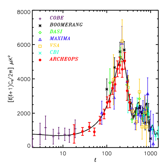
Figure 1: Measurements of the CMB angular power spectrum by Archeops (in red dots) compared with CBDMVC datasets. A $\Lambda$CDM model (see text for parameters) is overplotted and appears to be in good agreement with all the data.

2 Archeops angular power spectrum

The first results of the February 2002 flight of Archeops are detailed in Benoît et al. 2002 . The band powers used in this analysis are plotted in Fig. 1 together with those of other experiments (CBDMVC for COBE, Boomerang, Dasi, Maxima, VSA, and CBI; Tegmark et al. 1996 , Netterfield et al. 2002 , Halverson et al. 2002 , Lee et al. 2001 , Scott et al. 2002 , Pearson et al. 2002 ). Also plotted is a $\Lambda$CDM model (computed using CAMB, Lewis et al. 2000 ), with the following cosmological parameters: $\Theta=(\Omega_{\rm tot},\Omega_{\Lambda},\Omega_{\rm b}h^{2},h,n,Q,\tau)=(1.00,0.7,0.02,0.70,1.00,18\mu K,0.)$ where the parameters are the total energy density, the energy density of a cosmological constant, the baryon density, the normalized Hubble constant ($H_{0}=100\,h\rm\,km/s/Mpc$), the spectral index of the scalar primordial fluctuations, the normalization of the power spectrum and the optical depth to reionization, respectively. The predictions of inflationary motivated adiabatic fluctuations, a plateau in the power spectrum at large angular scales followed by a first acoustic peak, are in agreement with the results from Archeops and from the other experiments. Moreover, the data from Archeops alone provides a detailed description of the power spectrum around the first peak. The parameters of the peak can be studied without a cosmological prejudice (Knox et al. 2000 ; Douspis & Ferreira 2002 ) by fitting a constant term, here fixed to match COBE amplitude, and a Gaussian function of $\ell$. Following this procedure and using the Archeops and COBE data only, we find (Fig. 2) for the location of the peak $\ell_{\rm peak}=220\pm 6$, for its width $FWHM=192\pm 12$, and for its amplitude $\delta T=71.5\pm 2.0\,\rm\mu K$ (error bars are smaller than the calibration uncertainty from Archeops only, because COBE amplitude is used for the constant term in the fit). This is the best determination of the parameters of the first peak to date, yet still compatible with other CMB experiments.

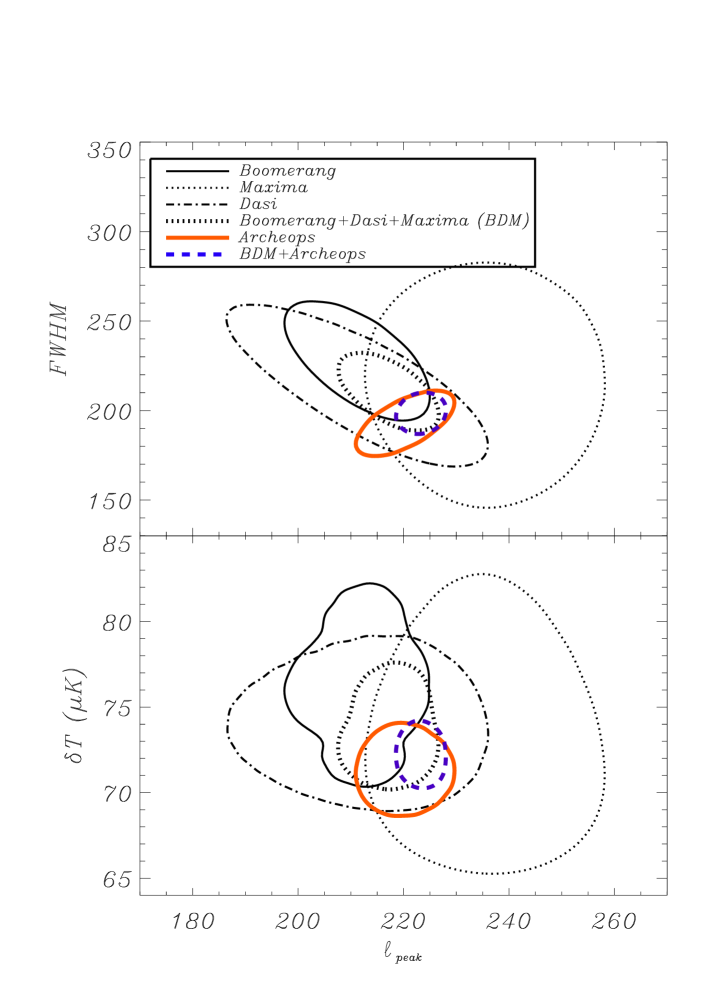
Figure 2: Gaussian fitting of the first acoustic peak using Archeops and other CMB experiments ($\ell\leq 390$). Top panel: 68% CL likelihood contours in the first peak position and FWHM ($\ell_{\rm peak},FWHM$) plane; Bottom panel: 68% CL likelihood contours in the first peak position and height ($\ell_{\rm peak},\delta T_{\rm peak}$) plane for different CMB experiments and combinations. The width of the peak is constrained differently by Archeops and BDM experiments, so that the intersection lies on relatively large $\ell_{\rm peak}$. Hence, the BDM + Archeops zone is skewed to the right in the bottom panel.

	$\Omega_{\rm tot}$	$\Omega_{\Lambda}$	$\Omega_{\rm b}h^{2}$	$h$	$n$	$Q$	$\tau$
Min.	0.7	0.0	0.00915	0.25	0.650	11	0.0
Max.	1.40	1.0	0.0347	1.01	1.445	27	1.0
Step	0.05	0.1	0.00366	*1.15	0.015	0.2	0.1

Table 1: The grid of points in the 7 dimensional space of cosmological models that was used to set constraint on the cosmological parameters. ^∗For $h$ we adopt a logarithmic binning: $h(i+1)=1.15\cdot h(i)$ ; $Q$ is in $\mu K$.

3 Model grid and likelihood method

To constrain cosmological models we constructed a $4.5\times 10^{8}$ $C_{\ell}$ database. Only inflationary motivated models with adiabatic fluctuations are being used. The ratio of tensor to scalar modes is also set to zero. As the hot dark matter component modifies mostly large $\ell$ values of the power spectrum, this effect is neglected in the following. Table 1 describes the corresponding gridding used for the database. The models including reionization have been computed with an analytical approximation (Griffiths et al. 1999 ).

Cosmological parameter estimation relies upon the knowledge of the likelihood function $\mathcal{L}$ of each band power estimate. Current Monte Carlo methods for the extraction of the $C_{\ell}$ naturally provide the distribution function $\mathcal{D}$ of these power estimates. The analytical approach described in Douspis et al. (2002) and Bartlett et al. 2000 allows to construct the needed $\mathcal{L}$ in an analytical form from $\mathcal{D}$. Using such an approach was proven to be equivalent to performing a full likelihood analysis on the maps. Furthermore, this leads to unbiased estimates of the cosmological parameters (Wandelt et al. 2001 , Bond et al. 2000 , Douspis et al. 2001a ), unlike other commonly used $\chi^{2}$ methods. In these methods, $\mathcal{L}$ is also assumed to be Gaussian. However this hypothesis is not valid, especially for the smaller modes covered by Archeops. The difference between our well–motivated shape and the Gaussian approximation induces a 10% error in width for large–scale bins. The parameters of the analytical form of the band power likelihoods $\mathcal{L}$ have been computed from the distribution functions of the band powers listed in Tab. 1 of Benoît et al. 2002 . Using $\mathcal{L}$, we calculate the likelihood of any of the cosmological models in the database and maximize the likelihood over the 7% calibration uncertainty. We include the calibration uncertainty of each experiment as extra parameters in our analysis. The prior on these parameters are taken as Gaussians centered on unity, with a standard deviation corresponding to the quoted calibration uncertainty of each dataset. The effect of Archeops beam width uncertainty, which leads to less than 5% uncertainty on the $C_{\ell}$’s at $\ell\leq 350$, is neglected.

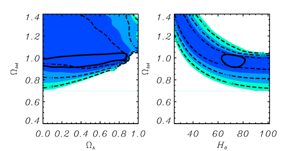
Figure 3: Likelihood contours in the $(\Omega_{\Lambda},\Omega_{\rm tot})$ (left) and $(H_{0},\Omega_{\rm tot})$ (right) planes using the Archeops dataset; the three colored regions (three contour lines) correspond to resp. 68, 95 and 99% confidence levels for 2-parameters (1-parameter) estimates. Black solid line is given by the combination Archeops + HST, see text.

A numerical compilation of all the results is given in Tab. 2. Some of the results are also presented as 2-D contour plots, showing in shades of blue the regions where the likelihood function for a combination of any two parameters drops to 68%, 95%, and 99% of its initial value. These levels are computed from the minimum of the negative of the log likelihood plus $\Delta=2.3,\;6.17\;\rm and\;11.8$. They would correspond to 1, 2, 3 $\sigma$ respectively if the likelihood function was Gaussian. Black contours mark the limits to be projected if confidence intervals are sought for any one of the parameters. To calculate either 1– or 2–D confidence intervals, the likelihood function is maximized over the remaining parameters. All single parameter confidence intervals that are quoted in the text are $1\,\sigma$ unless otherwise stated, and we use the notation $\chi^{2}_{gen}=m/n$ to mean that the generalized $\chi^{2}$ has a value $m$ with $n$ degrees of freedom. In all cases described below we find models that do fit the data and therefore confidence levels have a well defined statistical interpretation. Douspis et al. (2002) describes how to evaluate the goodness of fit and Tab. 2 gives the various $\chi^{2}$ values. When we use external non–CMB priors on some of the cosmological parameters, the analysis is done by multiplying our CMB likelihood hypercube by Gaussian shaped priors with mean and width according to the published values.

4 Cosmological Parameter constraints

4.1 Archeops

We first find constraints on the cosmological parameters using the Archeops data alone. The cosmological model that presents the best fit to the data has a $\chi^{2}_{gen}=6/9$. Figure 3 gives confidence intervals on different pairs of parameters. The Archeops data constrain the total mass and energy density of the Universe ($\Omega_{\rm tot}$) to be greater than 0.90, but it does not provide strong limits on closed Universe models. Fig. 3 also shows that $\Omega_{\rm tot}$ and $h$ are highly correlated (Douspis et al. 2001b ). Adding the HST constraint for the Hubble constant, $H_{0}=72\pm 8\rm\,km/s/Mpc$ (68% CL, Freedman et al. 2001 ), leads to the tight constraint $\Omega_{\rm tot}=0.96^{+0.09}_{-0.04}$ (full line in Fig. 3), indicating that the Universe is flat.

Using Archeops data alone we can set significant constraints neither on the spectral index $n$ nor on the baryon content $\Omega_{\rm b}h^{2}$ because of lack of information on fluctuations at small angular scales.

4.2 COBE, Archeops, CBI

We first combine only COBE/DMR, CBI and Archeops so as to include information over a broad range of angular scales, $2\leq\ell\leq 1500$, with a minimal number of experiments. The results are shown in Fig. 4, with a best model $\chi^{2}_{gen}=9/20$. The constraint on open models is stronger than previously, with a total density $\Omega_{\rm tot}=1.16^{+0.24}_{-0.20}$ at 68% CL and $\Omega_{\rm tot}>0.90$ at 95% CL. The inclusion of information about small scale fluctuations provides a constraint on the baryon content, $\Omega_{\rm b}h^{2}=0.019^{+0.006}_{-0.007}$ in good agreement with the results from BBN (O’Meara et al. 2001 : $\Omega_{\rm b}h^{2}=0.0205\pm 0.0018$). The spectral index $n=1.06^{+0.11}_{-0.14}$ is compatible with a scale invariant Harrison–Zel’dovich power spectrum.

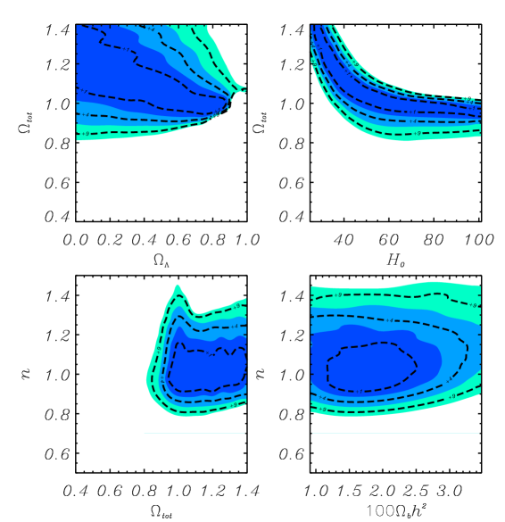
Figure 4: Likelihood contours for (COBE + Archeops + CBI) in the $(\Omega_{\Lambda},\Omega_{\rm tot})$, $(H_{0},\Omega_{\rm tot})$, $(\Omega_{\rm tot},n)$ and ($\Omega_{\rm b}h^{2},n$) planes.

4.3 Archeops and other CMB experiments

By adding the experiments listed in Fig. 1 we now provide the best current estimate of the cosmological parameters using CMB data only. The constraints are shown on Fig. 5 and 6 (left). The combination of all CMB experiments provides $\sim 10\%$ errors on the total density, the spectral index and the baryon content respectively: $\Omega_{\rm tot}=1.15^{+0.12}_{-0.17}$, $n=1.04^{+0.10}_{-0.12}$ and $\Omega_{\rm b}h^{2}=0.022^{+0.003}_{-0.004}$. These results are in good agreement with recent analyses performed by other teams (Netterfield et al. 2002 , Pryke et al. 2002 , Rubino-Martin et al. 2002 , Sievers et al. 2002 , Wang et al. 2002 ). One can also note that the parameters of the $\Lambda$CDM model shown in Fig. 1 are included in the 68% CL contours of Fig. 6 (right).

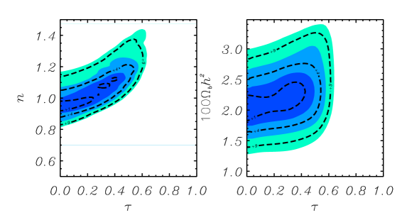
Figure 5: Likelihood contours in the $(\tau,n)$ and $(\tau,\Omega_{\rm b}h^{2})$ planes using Archeops + CBDMVC datasets.

As shown in Fig. 5 the spectral index and the optical depth are degenerate. Fixing the latter to its best fit value, $\tau=0$, leads to stronger constraints on both $n$ and $\Omega_{\rm b}h^{2}$. With this constraint, the prefered value of $n$ becomes slightly lower than 1, $n=0.96^{+0.03}_{-0.04}$, and the constraint on $\Omega_{\rm b}h^{2}$ from CMB alone is not only in perfect agreement with BBN determination but also has similar error bars, $\Omega_{\rm b}h^{2}_{\rm(CMB)}=0.021^{+0.002}_{-0.003}$. It is important to note that many inflationary models (and most of the simplest of them) predict a value for $n$ that is slightly less than unity (see, e.g., Linde 1990 and Lyth & Riotto 1999 for a recent review).

4.4 Adding non–CMB priors

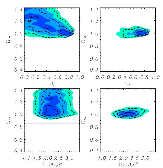
Figure 6: Likelihood contours in the $(\Omega_{\rm tot},\Omega_{\Lambda})$ and $(\Omega_{\rm tot},\Omega_{\rm b}h^{2})$ planes. Left: constraints using Archeops+CBDMVC datasets. Right: adding HST prior for $H_{0}$.

In order to break some degeneracies in the determination of cosmological parameters with CMB data alone, priors coming from other cosmological observations are now added. First we consider priors based on stellar candles like HST determination of the Hubble constant (Freedman et al. 2001 ) and supernovæ determination of $\Omega_{\rm m}$ and $\Lambda$ (Perlmutter et al. 1999 ). We also consider non stellar cosmological priors like BBN determination of the baryon content, (O’Meara et al. 2001 ), and baryon fraction determination from X-ray clusters (Roussel et al. 2000 , Sadat & Blanchard 2001 ). For the baryon fraction we use a low value, BF(L), $f_{b}=0.031h^{-3/2}+0.012\;(\pm 10\%)$, and a high value, BF(H), $f_{b}=0.048h^{-3/2}+0.014\;(\pm 10\%)$ (Douspis et al. 2001b and references therein). The results with the HST prior are shown in Figure 6 (right). Considering the particular combination Archeops + CBDMVC + HST, the best fit model, within the Tab. 1 gridding, is $(\Omega_{\rm tot},\Omega_{\Lambda},\Omega_{\rm b}h^{2},h,n,Q,\tau)=(1.00,0.7,0.02,0.665,0.945,19.2{\rm\mu K},0.)$ with a $\chi^{2}_{gen}=41/68$. The model is shown in Fig. 7 with the data scaled by their best–fit calibration factors which were simultaneously computed in the likelihood fitting process. The constraints on $h$ break the degeneracy between the total matter content of the Universe and the amount of dark energy as discussed in Sect. 4.1. The constraints are then tighter as shown in Fig. 6 (right), leading to a value of $\Omega_{\Lambda}=0.73^{+0.09}_{-0.07}$ for the dark energy content, in agreement with supernovæ measurements if a flat Universe is assumed. Table 2 also shows that Archeops + CBDMVC cosmological parameter determinations assuming either $\Omega_{\rm tot}=1$ or the HST prior on $h$ are equivalent at the 68% CL.

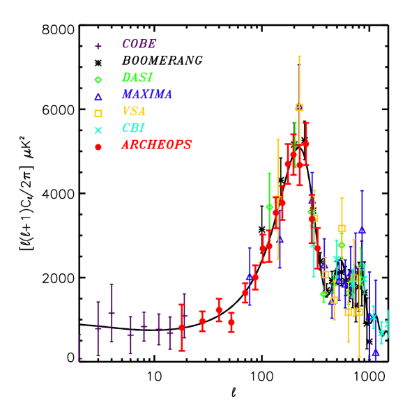
Figure 7: Best model obtained from the Archeops + CBDMVC + HST analysis with recalibrated actual datasets. The fitting allowed the gain of each experiment to vary within their quoted absolute uncertainties. Recalibration factors, in temperature, which are applied in this figure, are 1.00, 0.96, 0.99, 1.00, 0.99, 1.00, and 1.01, for COBE, Boomerang, Dasi, Maxima, VSA, CBI and Archeops respectively, well within 1 $\sigma$ of the quoted absolute uncertainties ($<1$, 10, 4, 4, 3.5, 5 and 7%).

Data	$\Omega_{\rm tot}$	$n_{s}$	$\Omega_{\rm b}h^{2}$	$h$	$\Omega_{\Lambda}$	$\tau$	$\chi^{2}_{gen}/dof$
Archeops	$>0.90$	$1.15^{+0.30}_{-0.40}$	$--$	$--$	$<0.9$	$<0.45$	$6/9$
Archeops + COBE + CBI	$1.16^{+0.24}_{-0.20}$	$1.06^{+0.11}_{-0.14}$	$0.019^{+0.006}_{-0.007}$	$>0.25$	$<0.85$	$<0.45$	$9/20$
CMB	$1.18^{+0.22}_{-0.20}$	$1.06^{+0.14}_{-0.20}$	$0.024^{+0.003}_{-0.005}$	$0.51^{+0.30}_{-0.30}$	$<0.85$	$<0.55$	$37/52$
Archeops + CMB	$1.15^{+0.12}_{-0.17}$	$1.04^{+0.10}_{-0.12}$	$0.022^{+0.003}_{-0.004}$	$0.53^{+0.25}_{-0.13}$	$<0.85$	$<0.4$	$41/67$
Archeops + CMB + $\tau=0$	$1.13^{+0.12}_{-0.15}$	$0.96^{+0.03}_{-0.04}$	$0.021^{+0.002}_{-0.003}$	$0.52^{+0.20}_{-0.12}$	$<0.80$	$0.0$	$41/68$
Archeops + CMB + $\Omega_{\rm tot}=1$	$1.00$	$1.04^{+0.10}_{-0.12}$	$0.021^{+0.004}_{-0.003}$	$0.70^{+0.08}_{-0.08}$	$0.70^{+0.10}_{-0.10}$	$<0.40$	$41/68$
Archeops + CMB + HST	$1.00^{+0.03}_{-0.02}$	$1.04^{+0.10}_{-0.08}$	$0.022^{+0.003}_{-0.002}$	$0.69^{+0.08}_{-0.06}$	$0.73^{+0.09}_{-0.07}$	$<0.42$	$41/68$
Archeops + CMB + HST + $\tau=0$	$1.00^{+0.03}_{-0.02}$	$0.96^{+0.02}_{-0.04}$	$0.021^{+0.001}_{-0.003}$	$0.69^{+0.06}_{-0.06}$	$0.72^{+0.08}_{-0.06}$	$0.0$	$41/69$
Archeops + CMB + SN1a	$1.04^{+0.02}_{-0.04}$	$1.04^{+0.10}_{-0.12}$	$0.022^{+0.003}_{-0.004}$	$0.60^{+0.10}_{-0.07}$	$0.67^{+0.11}_{-0.03}$	$<0.40$	$41/69$
Archeops + CMB + BBN	$1.12^{+0.13}_{-0.14}$	$1.04^{+0.10}_{-0.12}$	$0.020^{+0.002}_{-0.002}$	$0.50^{+0.15}_{-0.10}$	$<0.80$	$<0.25$	$41/68$
Archeops + CMB + BF(H)	$1.11^{+0.12}_{-0.11}$	$1.03^{+0.12}_{-0.14}$	$0.022^{+0.004}_{-0.004}$	$0.46^{+0.09}_{-0.11}$	$0.45^{+0.10}_{-0.10}$	$<0.40$	$43/69$
Archeops + CMB + BF(L)	$1.22^{+0.18}_{-0.12}$	$1.03^{+0.07}_{-0.13}$	$0.021^{+0.003}_{-0.004}$	$<0.40$	$<0.3$	$<0.40$	$45/69$

Table 2: Cosmological parameter constraints from combined datasets. Upper and lower limits are given for 68% CL. See text for details on priors. The central values are given by the mean of the likelihood. The quoted error bars are at times smaller than the parameter grid spacing, and are thus in fact determined by an interpolation of the likelihood function between adjacent grid points.

5 Conclusion

Constraints on various cosmological parameters have been derived by using the Archeops data alone and in combination with other measurements. The measured power at low $\ell$ is in agreement with the COBE data, providing for the first time a direct link between the Sachs–Wolfe plateau and the first acoustic peak. The Archeops data give a high signal-to-noise ratio determination of the parameters of the first acoustic peak and of the power spectrum down to COBE scales ($\ell=15$), because of the large sky coverage that greatly reduces the sample variance. The measured spectrum is in good agreement with that predicted by simple inflation models of scale–free adiabatic peturbations. Archeops on its own also sets a constraint on open models, $\Omega_{\rm tot}>0.90$ (68% CL). In combination with CBDMVC experiments, tight constraints are shown on cosmological parameters like the total density, the spectral index and the baryon content, with values of $\Omega_{\rm tot}=1.13^{+0.12}_{-0.15}$, $n=0.96^{+0.03}_{-0.04}$ and $\Omega_{\rm b}h^{2}=0.021^{+0.002}_{-0.003}$ respectively, all at 68% CL and assuming $\tau=0$. These results lend support to the inflationary paradigm. The addition of non–CMB constraints removes degeneracies between different parameters and allows to achieve a $10\%$ precision on $\Omega_{\rm b}h^{2}$ and $\Omega_{\Lambda}$ and better than 5% precision on $\Omega_{\rm tot}$ and $n$. Flatness of the Universe is confirmed with a high degree of precision: $\Omega_{\rm tot}=1.00^{+0.03}_{-0.02}$ (Archeops + CMB + HST).

- (1) Balbi, A., Ade, P., Bock, J., et al. 2000, ApJ, 545, L1
- (2) Bartlett, J. G., Douspis, M., Blanchard, A., & Le Dour, M. 2000, A&AS, 146, 507
- (3) Bennett, C. L., Halpern, M., Hinshaw, G., et al. 1997, 191st AAS Meeting, 29, 1353
- (4) Benoît, A., Ade, P., Amblard, A., et al. 2002, A&A, submitted astro-ph/0210305
- (5) Bond, J. R., Jaffe, A. H., & Knox, L. 2000, ApJ, 533, 19
- (6) de Bernardis, P., Ade, P. A. R., Bock, J. J., et al. 2000, Nature, 404, 955
- (7) Douspis, M., Bartlett, J. G. & Blanchard, A. & Le Dour, M. 2001a, A&A, 368, 1
- (8) Douspis, M., Blanchard, A., Sadat, R., et al. 2001b, A&A, 379, 1
- (9) Douspis, M. & Ferreira, P. 2002, Phys. Rev. D, 65, 87302
- Douspis et al. (2002) Douspis, M., et al. 2002, A&A, submitted
- (11) Freedman, W. L., Madore, B. F., Gibson, B. K., et al. 2001, ApJ, 553, 47
- (12) Griffiths, L. M., Barbosa, D., & Liddle, A. R. 1999, MNRAS, 308, 854
- (13) Halverson, N. W., Leitch, E. M., Pryke, C., et al. 2002, MNRAS, 568, 38
- (14) Hanany, S., Ade, P., Balbi, A., et al. 2000, ApJ, 545, L5
- (15) Hancock, S., Rocha, G., Lasenby, A. N., & Gutierrez, C. M. 1999, MNRAS, 294, L1
- (16) Knox, L. & Page, L. 2000, Phys.Rev.Lett., 85, 1366
- (17) Lange, A. E., Ade, P. A., Bock, J. J., et al. 2001, Phys. Rev. D, 63, 4, 042001
- (18) Lee, A. T., Ade, P., Balbi, A. et al. 2001, ApJ, 561, L1
- (19) Lewis, A., Challinor, A., & Lasenby, A. 2000, ApJ, 538, 473
- (20) Linde, A.D., 1990, Particle Physics and Inflationary Cosmology (Harwood Academic, N.Y., 1990)
- (21) Lineweaver, C. H., Barbosa, D., Blanchard, A., & Bartlett, J. G. 1997, A&A, 322, 365
- (22) Lyth, D. H. & Riotto, A. 1999, Phys.Rep., 314, 1
- (23) Netterfield, C. B., Devlin, M. J., Jarolik, N., et al. 1997, ApJ, 474, 47
- (24) Netterfield, C. B., Ade, P. A. R., Bock, J. J., et al. 2002, ApJ, 571, 604
- (25) O’Meara, J. M.; Tytler, D., Kirkman, D., et al. 2001, ApJ, 552, 718
- (26) Pearson, T. J., Mason, B. S., Readhead, A. C. S., et al. 2002, ApJ, submitted, astro-ph/0205388
- (27) Perlmutter, S., Aldering, G., Goldhaber, G., et al. 1999, ApJ, 517, 565 & http://www-supernova.lbl.gov
- (28) Pryke, C., Halverson, N. W., Leitch, E. M., et al. 2002, ApJ, 568, 46
- (29) Roussel, H., Sadat, R., & Blanchard, A. 2000, A&A, 361, 429
- (30) Rubino-Martin, J. A., Rebolo, R., Carreira, P., et al. 2002, astro-ph/0205367
- (31) Sadat, R., & Blanchard, A. 2001, A&A, 371, 19
- (32) Scott, P. F., Carreira, P., Cleary, K., et al. 2002, astro-ph/0205380
- (33) Seljak, U. & Zaldarriaga, M. 1996, ApJ, 469, 437
- (34) Sievers J. L., Bond, J. R., Cartwright, J. K., et al. 2002, ApJ, submitted, astro-ph/0205387
- (35) Tauber, J.A. et al. 2000, IAU Symp. 204, ed. M. Harwit & M. G. Hauser
- (36) Tegmark, M. 1996, ApJ, 464, L35
- (37) Wandelt, B. D., Hivon, E., & Górski, K. M. 2001, Phys. Rev. D, 64, 83003
- (38) Wang, X., Tegmark, M., & Zaldarriaga, M. 2002, Phys. Rev. D, 65, 123001