Abstract

We review the recently published results from the CBI’s first season of observations. Angular power spectra of the CMB were obtained from deep integrations of 3 single fields covering a total of 3 deg² and 3 shallower surveys of overlapping (mosaiced) fields covering a total of 40 deg². The observations show a damping of the anisotropies at high-$\ell$ as expected from the standard scenarios of recombination. We present parameter estimates obtained from the data and discuss the significance of an excess at $\ell>2000$ observed in the deep fields.

CMB observations with the Cosmic Background Imager (CBI) Interferometer

¹ Canadian Institute for Theoretical Astrophysics 60 St. George Street, Toronto Ontario M5S 3H8
² University of Alberta, ³ Caltech, ⁴ NRAO, ⁵ IAP, ⁶ University of Toronto, ⁷ McMaster University

1 Introduction

The CBI is an array of 13 0.9-meter diameter Cassegrain antennas mounted on a 6-meter diameter tracking platform. The results presented here are based on an analysis of data obtained from January through to December 2000 [6, 9]. Previous experiments such as BOOMERANG[8], DASI[4] and MAXIMA[5] have measured precisely the shape of a first peak at $\ell\sim 220$, consistent with an $\Omega_{tot}=1$ $\Lambda$CDM universe with adiabatic, inflationary seeded perturbations. A significant detection of a second peak has also been established [1] with evidence for a third. The CBI observations have now extended the multipole range observed by multiple band experiments by a factor of $3$. The results have confirmed another important element of the adiabatic, inflationary paradigm, the damping at high multipoles due to the viscous drag over the finite width of the last scattering surface [10]. Mason et al.(2002) [6] give a description of the CBI instrumental setup and observing strategy. Here we review the main results and cosmological parameter fits obtained from the observations and discuss the nature of the possible excess observed on the smallest angular scales at $2000<\ell<4000$.

2 Results

The instrument observes in 10 frequency channels spanning the band $26-36$GHz and measures 78 baselines simultaneously. Our power spectrum estimation pipeline is described in [7] and involves an optimal compression of the ${\cal O}(10^{5})$ visibility measurements of each field into a coarse grained lattice of visibility estimators. Known point sources are projected out of the data sets when estimating the primary anisotropy spectrum by using a number of constraint matrices. The positions are obtained from the (1.4GHz) NVSS catalog [3]. When projecting out the sources we use large amplitudes which effectively marginalize over all affected modes. This insures robustness with respect to errors in the assumed fluxes of the sources. The residual contribution of sources below our $S_{1.4}=3.4$ mJy cutoff is treated as a white noise background with an estimated amplitude of $0.08\pm 0.04$ Jy/sr${{}^{-}1}$ [6].

The power spectra for both the mosaic and deep observations are shown in Figure 1. Both show a clear detection of the expected damping of the power at $\ell>1000$.

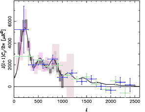
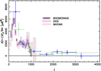
Figure 1: The mosaic (left) and deep (right) field power spectra. Two separate binnings of the data are shown (blue and green). We also include 1-sigma confidence intervals for the BOOMERANG, DASI and MAXIMA experiments. The hatched (grey) errors show the effect of the beam uncertainty on the BOOMERANG measurements. The solid curve in the left panel is a best fit spectrum to all the data shown.

We fit a minimal set of inflationary parameters to the data; $\omega_{b}=\Omega_{b}h^{2}$, $\omega_{\rm cdm}=\Omega_{\rm cdm}h^{2}$, $\Omega_{\Lambda}$, $\Omega_{tot}$, $n_{s}$, $\tau_{c}$. We also include calibration errors and beam errors where applicable. Our parameter fitting pipeline is described in detail in Sievers et al. (2002) [10]. The results for the combination of CBI and DMR data are shown in Table 1 for various combinations of priors. Our parameter fits and best fit models are consistent with previous results from fits to data at lower multipoles. We have also carried out a combined analysis of the CBI data with the BOOMERANG, MAXIMA and DASI data and with a compilation of data predating April 2001 [10].

Table 1: Parameter constraints from CBI+DMR for a selection of priors.

Priors	$\Omega_{tot}$	$n_{s}$	$\Omega_{b}h^{2}$	$\Omega_{\rm cdm}h^{2}$	$\Omega_{\Lambda}$	$\tau_{c}$
wk	$0.99^{0.12}_{0.12}$	$1.05^{0.09}_{0.08}$	$0.022^{0.015}_{0.009}$	$0.17^{0.08}_{0.06}$	$0.40^{0.25}_{0.27}$	$0.22^{0.19}_{0.16}$
wk+LSS	$1.01^{0.09}_{0.06}$	$1.02^{0.11}_{0.07}$	$0.026^{0.014}_{0.010}$	$0.12^{0.03}_{0.03}$	$0.64^{0.11}_{0.14}$	$0.14^{0.22}_{0.11}$
wk+SN	$1.02^{0.09}_{0.08}$	$1.07^{0.09}_{0.09}$	$0.027^{0.015}_{0.011}$	$0.12^{0.05}_{0.05}$	$0.70^{0.08}_{0.09}$	$0.24^{0.18}_{0.18}$
wk+LSS+SN	$1.00^{0.10}_{0.06}$	$1.06^{0.09}_{0.08}$	$0.027^{0.014}_{0.011}$	$0.12^{0.04}_{0.04}$	$0.70^{0.07}_{0.07}$	$0.21^{0.20}_{0.15}$
Flt+wk	(1.00)	$1.04^{0.10}_{0.08}$	$0.023^{0.010}_{0.008}$	$0.15^{0.06}_{0.04}$	$0.46^{0.22}_{0.29}$	$0.22^{0.19}_{0.16}$
Flt+wk+LSS	(1.00)	$1.01^{0.10}_{0.07}$	$0.025^{0.010}_{0.008}$	$0.13^{0.02}_{0.01}$	$0.64^{0.10}_{0.13}$	$0.15^{0.17}_{0.11}$
Flt+wk+SN	(1.00)	$1.06^{0.11}_{0.09}$	$0.026^{0.010}_{0.009}$	$0.13^{0.03}_{0.02}$	$0.69^{0.06}_{0.07}$	$0.22^{0.19}_{0.16}$
Flt+wk+LSS+SN	(1.00)	$1.05^{0.09}_{0.07}$	$0.027^{0.009}_{0.009}$	$0.13^{0.02}_{0.01}$	$0.70^{0.05}_{0.06}$	$0.20^{0.16}_{0.14}$
Flt+HST	(1.00)	$1.06^{0.10}_{0.08}$	$0.026^{0.010}_{0.009}$	$0.15^{0.07}_{0.04}$	$0.61^{0.10}_{0.21}$	$0.21^{0.19}_{0.16}$
Flt+HST+LSS	(1.00)	$1.04^{0.08}_{0.07}$	$0.027^{0.009}_{0.008}$	$0.13^{0.02}_{0.01}$	$0.68^{0.05}_{0.07}$	$0.19^{0.15}_{0.13}$
Flt+HST+SN	(1.00)	$1.06^{0.11}_{0.09}$	$0.027^{0.009}_{0.009}$	$0.13^{0.03}_{0.02}$	$0.69^{0.04}_{0.06}$	$0.22^{0.19}_{0.16}$
Flt+HST+LSS+SN	(1.00)	$1.05^{0.08}_{0.07}$	$0.027^{0.009}_{0.009}$	$0.13^{0.02}_{0.01}$	$0.70^{0.04}_{0.05}$	$0.20^{0.15}_{0.14}$

The deep field measurements reveal an apparent excess in the power at multipoles $\ell>2000$ over standard adiabatic, inflationary models with a significance of $3.1\sigma$. The excess is a factor of $4.5$ greater than the estimated contribution from a background of residual sources and the confidence limit includes a $50\%$ error in the value for the background flux density.

We have considered whether secondary anisotropies from the Sunyaev-Zeldovich effect may explain the observed excess [2]. We used four hydrodynamical simulations employing both Smoothed Particle Hydrodynamics (SPH) and Moving Mesh Hydrodynamics (MMH) algorithms with rms amplitudes $\sigma_{8}=1.0$ and $0.9$ to calculate the expected contribution to the angular power spectrum from the SZE. We find that both algorithms produce power consistent with the observed excess for $\sigma_{8}=1$.

The CBI power spectrum estimation pipeline has been tested extensively using accurate simulations of the observations with the exact $uv$-coverage and noise characteristics of the observed fields [7]. We used the SZ maps from the hydrodynamical codes as foregrounds in our simulations to test the Gaussian assumption implicit in the bandpower estimation algorithm in the presence of extended non-Gaussian foregrounds such as the SZE. We find that, for the amplitudes considered, the pipeline recovers the total power accurately or the 30 maps considered [2] including at scales $\ell>2000$ where the signal is dominated by the SZ foregrounds.

3 Conclusions

Our analysis of the CBI observations has yielded parameters consistent with the standard $\Omega_{tot}=1$, $\Lambda$CDM model. These results, based on measurements extending to much higher $\ell$ than previous experiments, provide a unique confirmation of the model. The dominant feature in the data is the decline in the power with increasing $\ell$, a necessary consequence of the paradigm which has now been checked. In summary under weak prior assumptions the combination of CBI and DMR data gives $\Omega_{tot}=1.01_{-0.06}^{+0.09}$, and $n_{s}=1.02_{-0.07}^{+0.11}$, consistent with inflationary models; $\Omega_{\rm cdm}h^{2}=0.12\pm 0.03$, and $\Omega_{\Lambda}=0.64_{-0.14}^{+0.11}$. With more restrictive priors, flat+weak-$h$+LSS, are used, we find $\Omega_{\rm cdm}h^{2}=0.13_{-0.01}^{+0.02}$, consistent with large scale structure studies; $\Omega_{b}h^{2}=0.025_{-0.008}^{+0.010}$, consistent with Big Bang Nucleosynthesis; $\Omega_{m}=0.37\pm 0.11$, and $\Omega_{b}=0.060\pm 0.020$, indicating a low matter density universe; $h=0.65_{-0.12}^{+0.12}$, consistent with the recent determinations of the Hubble Constant based on the recently revised Cepheid period-luminosity law; and $t_{0}=14.0_{-1.2}^{+1.2}$ Gyr, consistent with cosmological age estimates based on the oldest stars in globular clusters. The combination of CMB measurements and LSS priors also enables us to constrain the normalization $\sigma_{8}$. We find that for flat+weak-$h$+LSS priors we obtain $\sigma_{8}=0.89_{-0.10}^{+0.14}$. Thus it appears that the normalization required to explain the excess with the SZE is in the upper range of the independent result based on the primary CMB signal and LSS data.

The 2001 observing season data is now being analyzed. Although the data will double the overall integration time and area it is not expected to increase the confidence of the high-$\ell$ measurements. Follow-up surveys of the deep fields in the optical range and correlation with existing X-ray catalogs may establish whether the measurement is indeed a serendipitous detection of the SZE and will be part of future work. However, the observations have highlighted the potential for SZE measurements to constrain $\sigma_{8}$ via the highly sensitive dependence of the angular power spectrum to the amplitude of the fluctuations ${\cal C}^{SZ}\sim\sigma_{8}^{7}$, although precise calibration of the theories from either numerical or analytical methods are required to make such conclusions feasible[2]. The CBI is currently being upgraded with polarization sensitive antennas for the 2002/2003 observing season.

Acknowledgements.  This work was supported by the National Science Foundation under grants AST 94-13935, AST 98-02989, and AST 00-98734. Research in Canada is supported by NSERC and the Canadian Institute for Advanced Research. The computational facilities at Toronto are funded by the Canadian Fund for Innovation. We are grateful to CONICYT for granting permission to operate the CBI at the Chajnantor Scientific Preserve in Chile.

References

- [1] P. deBernardis et al., Ap.J.564, 559 (2002).
- [2] J. R. Bond et al., submitted to Ap.J.(astro-ph/0205386).
- [3] J. J. Condon et al., Ap.J.115, 1693 (1998).
- [4] N. W. Halverson et al., Ap.J.568, 38 (2002).
- [5] A. T. Lee et al., Phys. Rev. D561, L1 (2002).
- [6] B. Mason et al., submitted to Ap.J.(astro-ph/0205384).
- [7] S. T. Myers et al., submitted to Ap.J.(astro-ph/0205385).
- [8] B. Netterfield et al., Ap.J.571, 604 (2002).
- [9] T. J. Pearson et al., submitted to Ap.J.(astro-ph/0205388).
- [10] J. Sievers et al., submitted to Ap.J.(astro-ph/0205387).