A Model of the Temporal Variability of Optical Light from Extrasolar Terrestrial Planets

Abstract

The light scattered by an extrasolar Earth-like planet’s surface and atmosphere will vary in intensity and color as the planet rotates; the resulting light curve will contain information about the planet’s properties. Since most of the light comes from a small fraction of the planet’s surface, the temporal flux variability can be quite significant, $\sim 10-100\%$. In addition, for cloudless Earth-like extrasolar planet models, qualitative changes to the surface (such as ocean fraction, ice cover) significantly affect the light curve. Clouds dominate the temporal variability of the Earth but can be coherent over several days. In contrast to Earth’s temporal variability, a uniformly, heavily clouded planet (e.g. Venus), would show almost no flux variability. We present light curves for an unresolved Earth and for Earth-like model planets calculated by changing the surface features. This work suggests that meteorological variability and the rotation period of an Earth-like planet could be derived from photometric observations. The inverse problem of deriving surface properties from a given light curve is complex and will require much more investigation.

Department of Astrophysical Sciences, Princeton University, Peyton Hall - Ivy Lane, Princeton, NJ 08544

Institute for Advanced Study, Einstein Drive, Princeton, NJ 08540

Department of Astrophysical Sciences, Princeton University, Peyton Hall - Ivy Lane, Princeton, NJ 08544

Terrestrial planets around nearby stars are of enormous interest, especially any that orbit in habitable zones (surface conditions compatible with liquid water), since they might have global environments similar to Earth’s and even harbor life. NASA and ESA are now planning very challenging and ambitious space missions-Terrestrial Planet Finder and Darwin respectively-to detect and characterize terrestrial planets orbiting nearby Sun-like stars. Very different designs are being considered at both optical and mid-IR wavelengths, but all have the goal of spectroscopic characterization of the atmospheric composition including the capability to detect gases important for or caused by life on Earth (e.g. O₂, O₃, CO₂, CH₄ and H₂O). A mission capable of measuring these spectral features would have the signal-to-noise necessary to measure photometric variability of the unresolved planet. Photometry used to investigate a planet in less integration time than necessary for spectroscopy or could be done concurrently.

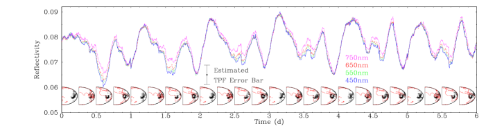
Figure 1.: Model light curve for Earth. The color of each line corresponds to the wavelength (450, 550, 650, 750 nm). The pictures below show the viewing geometry (continents outlined in red) and the amount of light contributed from each part of the surface (dark regions make largest contribution). Since cloud patterns produce the largest features in the light curve and are coherent over several days, the rotation period can determined and a daily average light curve can be calculated. Monte Carlo statistics produce the small “noise”. The small vertical jumps at three hour intervals is due to using discrete cloud cover maps.

In Fig. 1, we show the light curve of our Earth model for six consecutive days using cloud coverage obtained from satellite data. Photometric variations on the order of 20% could be easily detected by a TPF capable of spectroscopy.

Observations of the dark side of the Moon can be used to measure the reflectivity of the Earth (Goode et al. 2001). Fig. 2 (right) shows the viewing geometetry and illustrates why Earthshine observations are limited to certain viewing angles and times of day. Our model accurately reproduces both the mean reflectivity and the degree of variability (error bar at $90^{\circ}$ represents 1$\sigma$ variance between realizations) for widely separated days (See Fig. 2 left). The difference in magnitude of an extrasolar planet is given by

$$\Delta m=22.60+5\log\left(\frac{r}{AU}\right)-5\log\left(\frac{R_{p}}{R_{\oplus}}\right)-2.5\log\left(\mathcal{R}\right),$$ (1)

where $r$ is the star-planet distance, $R_{p}$ is the planet radius, and $\mathcal{R}$ is the reflectivity which varies with phase angle and viewing geometry.

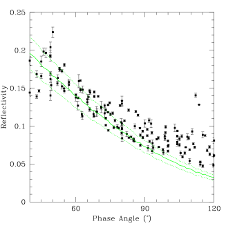
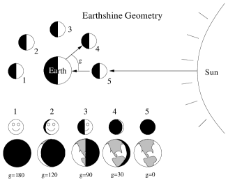
Figure 2.: Left: Comparison of model to Earthshine observations. Here we compare our Earth model (line) to the observations (points) taken near $90^{\circ}$ phase angle. Right: Viewing geometry for Earthshine observations.

The spectrum shown in Fig. 3 (left) illustrates a dramatic rise in reflectivity from the optical to the near-IR1 (see Fig. 3 left). Remote sensing satellites routinely use this feature to recognize vegetation on the Earth. The high reflectance at near-IR wavelengths is due to the arrangement of cells and air gaps in the leaves and is believed to allow plants to absorb light useful for photosynthesis while reflecting light which would only produce destructive excess heat.

We have used our Earth model to calculate the variation of Earth’s color using the actual distribution of clouds from satellite data and theoretical spectra from Traub & Jucks (2002) (see Fig. 3 right). The greater variability of the color centered on the red edge may be recognizable in Earthshine observations.

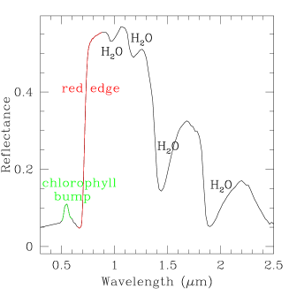
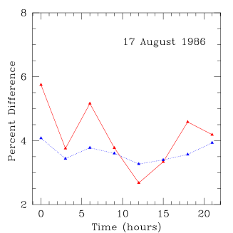
Figure 3.: Left: Spectrum of a deciduous leaf. The small bump comes from chlorophyll absorption bands on either side of 550nm and causes people to perceive plants as green. The much larger sharp rise (near 800nm, slightly beyond the optical) is known as the “red-edge”. Right: Variability of Earth’s color. The solid red line shows a color $\left(\frac{I(750-800\mathrm{nm})-I(700-650\mathrm{nm})}{I(750-800\mathrm{nm})}\right)$ chosen to emphasize variability due to vegetation’s red edge. For comparison, the dotted blue line shows a color $\left(\frac{I(850-800\mathrm{nm})-I(750-800\mathrm{nm})}{I(750-800\mathrm{nm})}\right)$ which is less sensitive to vegetation.

As the Earth rotates, different features rotate into view, causing significant variations in the total light from the entire planet. Once a rotation period is measured, observations over many rotation periods could be folded to obtain average light curves for summer, winter, and the entire year (see Fig. 4 left). We considered plausible cloudless Earth-like planets by altering the surface map of the Earth (see Fig. 4 right). While many of these qualitative surface changes result in significant changes to the light curves, deducing the surface of an extrasolar planet from its light curve could be quite difficult.

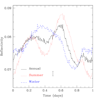
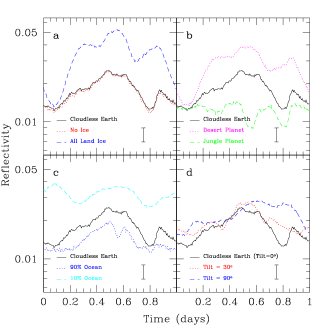
Figure 4.: Left: Model seasonal average light curves of cloudy Earth. Here the differences between the light curves are solely due to seasonal changes in the average cloud conditions, since changes in the snow cover is not included in the model. Detecting seasonal changes in a planet’s light curve could provide information about seasons. Interpretation could be complicated by changes in the viewing geometry. Right: Model for cloudless Earth-like planets. We consider plausible Earth-like planets by altering the surface map of the Earth. In panel a all the land is covered with ice or all the ice is replaced with desert. In panel b all the land is covered with thick forest or desert. In panel c the fraction of the surface covered with oceans is varied. All the above light curves have significant variability, $\sim 10-100\%$. Since qualitative changes to the surface significantly affect the light curve, the light curve may constrain surface properties. In panel d we consider the cloudless Earth for different obliquities.

References

Ford, E.B., Seager, S., & Turner, E.L. 2001, Nature 412: 6850, 885-886

Goode, P.R., Qui, J., Yurchyshyn, V., Hickey, J., Chu, M-C., Kolbe, E., Brown, C.T., & Koonin, S.E. 2001, Geophysical Research Letters 28: 9, 1671-1674

Schafer, J.P. & Turner, E.L. 2002, this proceedings 2H.2

Traub, W.A. & Jucks, K.W. 2002, AGU Geophysical Monograph, 130, 369