Abstract

Understanding the nature of the dark energy is one of the most important task in cosmology. In principle several cosmological observations can be used to discriminate amid a static cosmological constant contribution and a dynamical quintessence component. In view of the upcoming high resolution CMB experiments, using a model independent approach we study the dark energy imprint in the CMB anisotropy power spectrum and the degeneracy with other cosmological parameters.

Dark energy effects in the Cosmic Microwave Background Radiation

¹Centre for Theoretical Physics, University of Sussex, BN1 9QH, Falmer, Brighton, United Kingdom

1 Dark energy models

Two competitive scenarios have been proposed to take into account for the observed accelerated expansion of the universe [1], the cosmological constant and a plethora of ‘quintessence’ scalar field models. It has been recently shown that an appropriate parameterization of the time behavior of the dark energy equation of state, can reproduce the dynamics of several quintessence potentials and many other models for the acceleration [2]. In particular different models are specified by the value of the equation of state today $w_{Q}^{o}$, its value during the matter dominated era $w_{Q}^{m}$, the value of the scale factor $a_{c}^{m}$ where the equation of state changes from $w_{Q}^{o}$ to $w_{Q}^{m}$ and the width $\Delta$ of this transition. We refer to the formula (4) of the equation of state in reference [2]. We may distinguish two different classes of dark energy models, those with a rapid transition, characterized by the ratio $a_{c}^{m}/\Delta>1$, and those with a slowly varying behavior, for which $0<a_{c}^{m}/\Delta<1$. For instance the ‘Albrecht-Skordis’ model [3] belongs to the former class while the latter includes the inverse power law potential [4]. We shall study the dark energy effects in the CMB power spectrum and we will discuss the possibility to detect these imprints with the next generation of CMB experiments.

2 Acoustic peaks

The angular size of the sound horizon at the decoupling sets the location of the acoustic peaks. Different dark energy models can lead to a different angular diameter distance to the last scattering surface and consequently to a shift of the peaks. For instance if $w_{Q}^{o}$ is close to the cosmological constant value, the universe starts to accelerate at earlier times, the distance to the last scattering surface is farther and the peaks are shifted toward larger multipoles. The opposite effect occurs if $w_{Q}^{m}$ tends to the dust value or if $a_{c}^{m}$ tends to its present value $a_{o}=1$, but in these cases the amplitude of the shift depends on the value of $\Delta$. In fig.1 we plot the relative difference to a $\Lambda$CDM model of the position of the first, second and third peaks for rapidly varying models (fig.1a-1b) and slowly varying ones (fig.1c-1d). We set $w_{Q}^{o}=-1$. As we can see, in models with a rapidly varying equation of state the discrepancy with respect to the $\Lambda$CDM increases for $a_{c}^{m}\approx 1$ (fig.1a), while for slowly varying behaviors of the equation of state there is not dependence on $a_{c}^{m}$ (fig.1c). This is what we expect since in the latter class of models a different value of $a_{c}^{m}$ does not affect the evolution of the dark energy density. We notice that in general the shift of the position of the first peak is always larger than that of the second and third ones. This is due to the ISW effect that is a characteristic signature of dark energy at low multipoles.

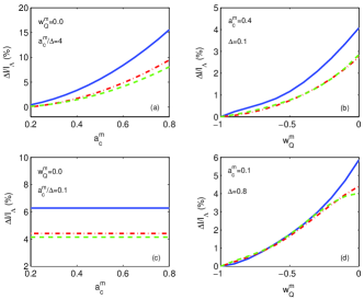
Figure 1: Relative difference of $l_{1}$ (blue solid line), $l_{2}$ (green dashed line) and $l_{3}$ (red dash-dotted line) to the $\Lambda$CDM model, for rapidly varying models ($top$ $panels$), and with slow transition ($bottom$ $panels$). For these models the present value of the equation of state is $w_{Q}^{o}=-1$.

The location of the Doppler peaks is an efficient tool to test the dark energy [5], however we should consider the degeneracy with other cosmological parameters. For example, for small values of $H_{o}$ the peaks are shifted toward large multipoles. The same effect occurs for large values of the physical baryon density $\Omega_{b}$, since the size of the sound horizon becomes smaller. Therefore we expect the value of the dark energy parameters to be degenerate mainly with $H_{o}$ and $\Omega_{b}$.

3 ISW effect

The ISW produces late time anisotropies at the large angular scales of the CMB and is caused by the decay of the gravitational potentials [6]. In a $\Lambda$CDM model such a decay starts as soon as the universe enters in the cosmological constant dominated phase. On the other hand the quintessence contributes to this decay not only with the dynamics of the background but with its clustering properties as well. In fact the quintessence is not a smooth component, it has fluctuations that can cluster at the very large scales and modify the evolution of the matter perturbations. Therefore the imprint of the dark energy in the ISW depends on its specific features [7]. In fig.2 we plot the power spectrum $C_{l}^{ISW}$ for the models of fig.1, the red line corresponds to the ISW contribution in a $\Lambda$CDM model. As we can see, for rapidly varying models, there is a boost of power for transitions occurring at close redshifts (fig.2a). The $C_{l}^{ISW}$ then decreases toward the cosmological constant case as the transition moves at higher redshifts (fig.2a). The largest amplitude is obtained for $w_{Q}^{m}=0.0$, but the signal is suppressed for $w_{Q}^{m}<0.0$ (fig.2b). In the case of slowly varying models the ISW is almost independent of $a_{c}^{m}$ (fig.2c). It is larger than the $\Lambda$CDM for $w_{Q}^{m}=0.0$, becomes smaller for negative values of $w_{Q}^{m}$ and tends to the $\Lambda$ case for $w_{Q}^{m}<-0.3$ (fig.2d). The result of this qualitative analysis suggests that amid the dark energy models with $w_{Q}^{o}$ close to $-1$, those with a rapid transition occurring at low redshifts produce the most distinctive signature in the CMB power spectrum. On the contrary those with a slowly varying behavior are more difficult to distinguish from a cosmological constant model.

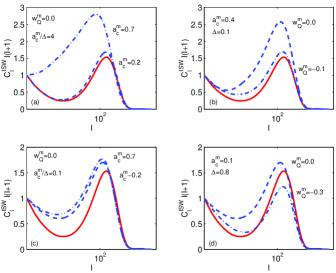
Figure 2: Power spectrum of the ISW for rapidly varying models ($top$ $panels$) and slowly varying ones ($bottom$ $panels$). The solid red line is the ISW effect produced in $\Lambda$CDM case.

4 Ideal CMB measurements

In order to test the sensitivity of an ideal CMB experiment to the dark energy effects, we simulate a sample of $C_{l}$s with cosmic variance errors. We assume a fiducial model with a slowly varying equation of state with the following parameters: $\Omega_{Q}=0.68$, $H_{o}=70$ Km $s^{-1}$ $Mpc^{-1}$, $w_{Q}^{o}=-1$, $w_{Q}^{m}=-0.4$, $a_{c}^{m}=0.2$, $\Delta=0.3$. We assume a flat geometry, no tensor contribution, the scalar spectral index $n=1$ and the baryon density $\Omega_{b}h^{2}=0.021$. We assume a gaussian prior on $\Omega_{m}=1-\Omega_{Q}$ with $\sigma_{m}=0.05$. We perform a likelihood analysis over $\Omega_{Q}$, $H_{o}$, $w_{Q}^{o}$, $w_{Q}^{m}$ and $a_{c}^{m}$. The results are shown in fig.3. As we may note, unless we take a prior on $H_{o}$, the value of $w_{Q}^{o}$ is poorly constrained. More important is the likelihood plot in the $w_{Q}^{m}-a_{c}^{m}$ plane. As we expect, $a_{c}^{m}$ is undetermined. On the other hand $w_{Q}^{m}$ is not very well constrained even with the $H_{o}$ prior. This is because $w_{Q}^{o}$ and $w_{Q}^{m}$ are degenerate, hence marginalizing the likelihood over $w_{Q}^{o}$ shifts the best fit value of $w_{Q}^{m}$. In particular we cannot exclude the case $w_{Q}^{m}=-1$. Therefore we conclude that if the present value of the dark energy equation of state is close to $-1$, a large class of models will not be distinguished from a $\Lambda$CDM scenario even with ideal CMB measurements. It is possible that combining different cosmological data, as SN Ia, large scale structure and quasar clustering we can break the degeneracy and infer more information on this class of dark energy models.

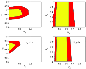
Figure 3: Simulated 2-D likelihood contour plots for an ideal experiment, with no priors ($top$ $panels$) and $H_{o}$ prior ($bottom$ $panels$). The yellow and red contours correspond to $1$ and $2\sigma$ respectively.

Acknowledgements.  We are grateful to Bruce Bassett, Carlo Ungarelli and Ed Copeland, with whom much of the work reviewed here has been done. PSC is suported by a University of Sussex bursary.

References

- [1] Perlmutter, S et al., 1999, ApJ 517, 565
- [2] Corasaniti, P. S. and Copeland, E. J., 2002, astro-ph/0205544
- [3] Albrecht, A., and Skordis, C. 1999, Phys. Rev. Lett. 84, 2076
- [4] Zlatev, I., Wang, L., and Steinhardt, P. J. 1999, Phys. Rev. Lett. 82, 896
- [5] Doran, M., Lilley, M. J., 2002, Mon. Not. Roy. Astron. Soc., 330, 965
- [6] Rees, M. J. and Sciama, D.W. 1968, Nature 217, 511
- [7] Corasaniti, P. S., Bassett, B. A., Ungarelli, C. and Copeland, E. J., astro-ph/0210209