Galaxy Star-Formation as a Function of Environment in the Early Data Release of the Sloan Digital Sky Survey1
Abstract
We present in this paper a detailed analysis of the effect of environment on the star–formation activity of galaxies within the Early Data Release (EDR) of the Sloan Digital Sky Survey (SDSS). We have used the H emission line to derive the star–formation rate (SFR) for each galaxy within a volume-limited sample of 8598 galaxies with and . We find that the SFR of galaxies is strongly correlated with the local (projected) galaxy density and thus we present here the density–SFR relation that is analogous to the density–morphology relation. The effect of density on the SFR of galaxies is seen in three ways. First, the overall distribution of SFRs is shifted to lower values in dense environments compared with the field population. Second, the effect is most noticeable for the strongly star–forming galaxies (H EW Å) in the 75th percentile of the SFR distribution. Third, there is a “break” (or characteristic density) in the density–SFR relation at a local galaxy density of . To understand this break further, we have studied the SFR of galaxies as a function of clustercentric radius from clusters and groups objectively selected from the SDSS EDR data. The distribution of SFRs of cluster galaxies begins to change, compared with the field population, at a clustercentric radius of – virial radii (at the statistical significance), which is consistent with the characteristic break in density that we observe in the density–SFR relation. This effect with clustercentric radius is again most noticeable for the most strongly star–forming galaxies.
Our tests suggest that the density-morphology relation alone is unlikely to explain the density–SFR relation we observe. For example, we have used the (inverse) concentration index of SDSS galaxies to classify late–type galaxies and show that the distribution of the star–forming (EW H Å) late–type galaxies is different in dense regions (within 2 virial radii) compared with similar galaxies in the field. However, at present, we are unable to make definitive statements about the independence of the density–morphology and density–SFR relation.
We have tested our work against potential systematic uncertainties including stellar absorption, reddening, SDSS survey strategy, SDSS analysis pipelines and aperture bias. Our observations are in qualitative agreement with recent simulations of hierarchical galaxy formation that predict a decrease in the SFR of galaxies within the virial radius. Our results are in agreement with recent 2dF Galaxy Redshift Survey results as well as consistent with previous observations of a decrease in the SFR of galaxies in the cores of distant clusters. Taken all together, these works demonstrate that the decrease in SFR of galaxies in dense environments is a universal phenomenon over a wide range in density (from to ) and redshift (out to ).
1 Introduction
In this paper, we investigate the relation between environment and star formation rate (SFR) of nearby galaxies. Spectroscopic studies of distant clusters of galaxies () have already established a clear connection between these two physical properties, in that the SFR of galaxies in the cores of distant clusters are significantly lower than those observed in the field at the same redshift (Balogh et al., 1997; Hashimoto et al., 1998; Poggianti et al., 1999; Couch et al., 2001; Postman et al., 2001). In particular, Balogh et al. (1998) found that the SFRs of cluster galaxies were lower relative to field galaxies of similar bulge-to-disk ratio, physical disk size, and luminosity, which suggests that the observed decrease in the star–formation may not be fully explained by the density–morphology (Dressler, 1980) or radius–morphology (Whitmore et al., 1993) relations (see also Poggianti et al. (1999); Couch et al. (2001); Balogh et al. (2002a)). This conclusion has also been suggested by Hashimoto et al. (1998), who used the Las Campanas Redshift Survey (LCRS) to study the relationship between local galaxy density, SFR, and galaxy concentration index, and found that cluster galaxies have a reduced level of SFR compared with the field, regardless of their concentration index. All these studies provide circumstantial evidence that galaxies are undergoing a physical transformation as they enter dense environments, and that the timescale for this transformation is different for the morphological and star formation properties.
In models of hierarchical galaxy formation (Kauffmann et al., 1993; Somerville & Primack, 1999; Cole et al., 2000), it is assumed that galaxies accreted into larger halos (e.g., they fall into groups or clusters) have their hot gas reservoir removed, which results in a gradual decline of the star–formation activity of galaxies in dense environments. This simple prescription is able to successfully match some of the general observed trends (Baugh et al., 1996; Diaferio et al., 2001; Balogh et al., 2000). At present, however, these models do not explore the physical details of how the galaxies lose their gas (see Bekki, Shioya & Couch 2002). Many possible mechanisms are proposed in the literature, such as ram pressure stripping of the cold gas due to interaction with the intracluster medium (Gunn & Gott, 1972; Quilis et al., 2000), galaxy harassment from high velocity encounters with other galaxies (Moore et al., 1999), tidal disruption (Byrd & Valtonen, 1990) or galaxy evolution via mergers and close encounters in in-falling poor groups (Zabludoff et al., 1996; Zabludoff & Mulchaey, 1998). Proper treatment of these effects will likely affect the details of the predicted relationships between galaxy properties and environment, but the relative importance of the proposed evolutionary mechanisms can only be determined with better data than has been available so far.
As a first step in addressing these issues, we use the Early Data Release (EDR; Stoughton et al. 2002) of the Sloan Digital Sky Survey (SDSS; see York et al., 2000) to further understand the relation between environment and the star–formation rate of galaxies. The EDR is an excellent database for such a study because it provides a large, homogeneous sample of galaxies, with medium resolution, flux–calibrated spectra and 5 passband photometry, over a wide range of environments. Such data allow for the computation of the H and [Oii] equivalent widths (EW) and SFR for all galaxies in a self–consistent way. Our work expands upon earlier cluster studies, as discussed above, in four key ways. First, we probe the rarefied field and poor group regimes, which include the most common galactic environments in the Universe. Second, we focus on the low redshift universe (), which provides a zero–point for the high redshift studies. Third, we are able to follow the star–formation of galaxies continuously from the cores of rich clusters and poor groups into the rarefied field. Finally, we can accurately quantify the local galaxy density in a uniform manner that is not subject to statistical background or luminosity corrections. Our work is complementary to earlier field studies using the 2dF Galaxy Redshift Survey (2dFGRS, see Lewis et al., 2002) and the LCRS (Hashimoto et al., 1998) and explores the density–SFR relation in greater detail than these previous works.
In Section 2, we present a description of the SDSS EDR data, the sample selection, and our SFR measurements. Our results are presented in Section 3. In Section 4, we discuss possible systematic biases, the density–morphology relation, and models of hierarchical structure formation. We also compare our work with previous studies, e.g., the 2dFGRS. In Section 5, we present our conclusions. In the Appendix, we discuss the details of selecting clusters and groups from the SDSS data. We also consider the effects of systematic biases that may influence our results, including the internal reddening of galaxies, sample selection, data analysis pipelines, and luminosity and aperture biases. Throughout this paper, we use , and unless otherwise stated.
2 Data
2.1 Early Data Release of the Sloan Digital Sky Survey
The Sloan Digital Sky Survey (http://www.sdss.org) is a 5 passband (, , , , ) imaging and medium–resolution () spectroscopic survey of the Northern Galactic Hemisphere (see York et al., 2000, for details). For technical details regarding the SDSS imaging survey, the reader is referred to Gunn et al. (1998), Smith et al. (2002), Pier et al. (2002) and Hogg et al. (2002). In June 2001, the SDSS publicly released photometric and spectroscopic data comprise of nearly 50,000 spectra of galaxies, stars and QSOs over 460 of sky. This release is known as the Early Data Release (EDR) and is fully described in Stoughton et al. (2002).
One of the unique features of the SDSS is the set of sophisticated data analysis software pipelines (see Lupton et al., 2001, Stoughton et al. 2002 for details) used to reduce the raw images and spectra into large catalogs of sources. Briefly, for each flux–calibrated SDSS spectrum, a redshift is determined both from the absorption lines (via cross-correlation; Heavens 1993) and the emission lines (via a wavelet–based peak–finding algorithm; Frieman et al. in prep). Once the redshift is known, the spectroscopic pipeline estimates the continuum emission at each pixel using the median value from a sliding box of 100 pixels (Å) centered on that pixel. Emission and absorption lines are measured through the fitting of a Gaussian, above the best–fit continuum, at the redshifted rest–wavelength of the lines. In order to accommodate line blending, the SDSS pipeline fits multiple Gaussians in the case of the H and [Nii] doublet and the [OIII] doublet. Thus, for all the major emission/absorption lines in the galaxy spectra, the spectroscopic pipeline provides an estimate of the equivalent width (EW), the continuum level (at center of the line), a line identification (e.g., H ), a goodness–of–fit (), and the height and sigma of the fitted Gaussian (and the associated statistical errors on all these quantities). These quantities are measured for all the major stellar emission and absorption lines regardless of their formal detection. In the Appendix, we present preliminary quality assurance tests of these emission line measurements which show that the H and [Oii] fluxes and EWs are robust.
When converting magnitude to flux, we have ignored the asinh magnitudes of Lupton et al. (1999) and treated the SDSS–EDR Petrosian magnitudes as traditional AB magnitudes (Fukugita et al., 1996). At the bright magnitudes used herein, the difference between these two magnitude systems is less than 1%, i.e., less than the photometric accuracy of the SDSS (see Stoughton et al. 2002).
2.2 Sample Selection
The reader is referred to Strauss et al. (2002) for a detailed description of the spectroscopic target selection for the SDSS main galaxy survey. For the analyses presented in this paper, we have used the EDR data discussed above but with the following additional selection criteria. We begin with all objects that have been spectroscopically confirmed as galaxies and have a redshift confidence of (see Heavens 1993). These criteria result in a sample of 41,622 galaxies. We then reject 37 objects that have certain redshift warning flags set in the database, i.e., we exclude spectra with the Z_WARNING_NO_BLUE (no blue side of the spectrum) and Z_WARNING_NO_RED (no red side of the spectrum) flags (see Stoughton et al. 2002). We also reject 1231 galaxies because they are duplicates. We have excluded another 37 galaxies that have , as these are likely spurious detections in the SDSS (see Table 21 of Stoughton et al., 2002), and, at this magnitude, the effect of the asinh magnitudes starts to become noticeable. This selection leaves us with 40,317 galaxies. Finally, we exclude 4014 galaxies for which the H emission line could not have been measured and 3452 galaxies for which the [Oii] emission could not have been measured. This is because these emission lines fall in masked regions of the spectrum, due to cosmic ray hits, cosmetic defects in the CCDs or missing data.
We define a volume-limited sample by further restricting the sample to galaxies in the redshift range and more luminous than (k–corrected, for ). This magnitude limit corresponds to , assuming from Blanton et al. (2001). The lower redshift limit is imposed to minimize aperture bias (see the Appendix), while the upper limit is the redshift where our luminosity limit equals the magnitude limit of the SDSS (; Strauss et al. 2002). These cuts leave us with a volume–limited sample 8598 galaxies for our analyses and includes all types of galaxies, not just emission line objects.
2.3 Measuring the Star–Formation Rate in Galaxies
The star formation rates of galaxies can be indirectly determined in various ways, as reviewed by Kennicutt (1998a). The most successful methods rely on correlations of the star formation rate with measurements of the far-infrared luminosity (which arises from dust heated by star formation), the radio luminosity (which results from synchroton emission associated with supernovae) and indicators that are sensitive to the ionizing flux from massive stars. The last category includes measurements of the ultraviolet continuum and the fluxes of nebular emission lines. Each of these techniques is subject to different biases and calibration uncertainties, but does give consistent estimates for “normal” galaxies when these effects are accounted for (Charlot et al., 2001; Hopkins et al., 2001; Sullivan et al., 2001). In this paper we focus on SFRs estimated from the H line. We also present the [Oii] EW measurements to facilitate comparison with high redshift studies of galaxies. Both lines are sensitive to the metallicity and ionization levels of the gas, though the problem is more significant for [Oii]. Dust extinction is the largest source of uncertainty, as both the effective optical depth and dust geometry must be considered (Charlot & Longhetti, 2001).
In Figure 1, we show the distribution of rest–frame H and [Oii] EWs, for the sample of galaxies discussed above. There is a small tail of negative EWs caused by statistical errors and, in the case of H , stellar absorption. Typically, stellar absorption is expected to account for Å of the H EW (Kennicutt, 1992; Charlot et al., 2001) and is therefore a small contribution to the majority of the strong emission line galaxy spectra (see the Appendix for more details). The distributions of [Oii] and H EWs are highly asymmetrical, skewed to low values but with a long tail to large, positive values. The observed mean of the SDSS [Oii] distribution (see Figure 1) is half the value of the observed mean for the field galaxy sample of the CNOC1 distant cluster studies (Balogh et al., 1997). This difference may be due to the differences in the apertures used by the SDSS and CNOC (although at z=0.1 the SDSS aperture corresponds to 5.5 kpc, while at z=0.3 the CNOC aperture corresponds to 6.7 kpc), or the evolution in the SFR of field galaxies (Lilly et al., 1996).
We have derived SFRs for these galaxies using the H flux (as computed from the pipeline output) and the theoretical relation from Kennicutt (1998b),
| (1) |
where is the observed luminosity in the H line (in erg ). This relation is valid for so-called Case B (optically thin) recombination, with a Salpeter (1955) initial mass function. We make no correction for negative SFRs that are caused by the small tail of negative H EWs in Figure 1. Although nonphysical, the negative SFR of these galaxies are included when computing the median, 25th, and 75th percentiles of the SFR distributions because removing them, or setting them to zero, would artificially skew the distributions. Alternatively, we could add a constant amount of stellar absorption to our sample but this would still leave a small negative tail, due to statistical errors, and the exact amount of stellar absorption to add remains unclear (see Appendix). We note here that the SFRs presented in this paper are not corrected for the 3 arcsecond SDSS fiber aperture and are therefore, systematically lower, by a factor of , compared to total SFRs derived from the radio or by integrating the light from the whole galaxy (see Hopkins et al., in prep)
We then correct the SFR for SFR–dependent reddening using the empirical formulae of Hopkins et al. (2001). We have also computed the normalized SFR (SFRN; see Postman et al., 2001), which is the observed SFR divided by the luminosity of each galaxy in our sample, i.e., where is the k–corrected ( magnitudes) AB –band luminosity (in Å-1 at the effective wavelength of the filter, Å) computed via the prescription outlined in Fukugita et al. (1996). To make the units more intuitive, we have re–normalized the luminosities by the characteristic AB luminosity from Blanton et al. (2001), i.e., Å-1. As discussed in Postman et al. (2001), such near–IR luminosities are less affected by recent star–formation and k–corrections and are more representative of the underlying stellar mass of the galaxy (at a given redshift) than are luminosities measured in bluer bands. The SFRN is therefore approximately the SFR per unit stellar luminosity, which helps to remove any large luminosity (or mass) bias from our results. We have also investigated the z-band luminosity function (LF) as a function of galaxy density and find, for the narrow range of bright z-band luminosities covered in this study, that the LF remains unchanged (within the errors) as a function of local galaxy density. This demonstrates that our results are unaffected by possible changes in the luminosity function of galaxies with local galaxy density.
3 Results
In this section, we present the results of two analyses of the relation between environment and the star–formation rate of galaxies. The first is an investigation of how the distribution of galaxy SFRs changes as a function of local (projected) density. This analysis spans over two orders of magnitude in density, from the rarefied field () to the densest environments (). The second analysis focuses only on virialized systems with velocity dispersions ranging from to and investigates the SFR of member galaxies as a function of clustercentric radius.
3.1 SFR as a Function of Local Galaxy Density
We investigate the SFR of galaxies as a function of their local galaxy density. We can parameterize the local environment of each galaxy using the projected density of galaxies in a manner similar to that employed by Dressler (1980). This involves calculating the projected distance to the 10th nearest spectroscopically–observed neighbor, and then converting that into a surface density (). As discussed in Section 2.2, our limit is (), which is close to the limit used by Dressler (, ). Our methodology does differ from that used by Dressler (1980) in that we use a circular search aperture (instead of a rectangle) and spectroscopically eliminate foreground and background galaxies so no further background correction is necessary. Thus our tenth nearest neighbor will be farther away than obtained via Dressler’s definition. Therefore, our effective “smoothing” scale is larger, and we may not be as sensitive as Dressler (1980) to the densest environments, i.e., cluster cores.
When calculating the local density, edge effects are particularly important because the EDR geometry is long strips of data that, at the median redshift of our sample, subtend only Mpc on the sky. To account for this, we remove any galaxy in which less than 75% of the circular area including the nearest neighbor lies within the EDR boundary. This corrections removes 1972 galaxies, leaving us with 6626 galaxies for our analysis. We do not make an area correction to our density estimates because we do not know if the nearest neighbor we have observed is, in fact, the true nearest neighbor. If it is, then correcting the density estimates for the area outside the survey boundary would bias the density estimates of those galaxies. Instead, we accept the fact that % of galaxies near the edge of the survey have an incorrect local density measurement but that they are not systematically biased. We have checked the effect of changing our tolerance to accepting galaxies near the edge of the survey, from rejecting all galaxies where the nearest neighbor is closer than any survey boundary, to including all galaxies regardless of edge effects, and find our results are robust.
In Figure 2, we show the distribution of local galaxy densities for the 6626 galaxies that satisfy this constraint. These local galaxy density measurements are significantly lower than those presented by Dressler (1980) and Dressler et al. (1997). These differences are partly due to the cosmologies used, the definitions of the field and search area (see above), differences in the edge corrections, and probable errors in the magnitudes used by Dressler (1980), which have uncertainties of at least 0.5 magnitudes. However, the most dominant effect is that we are probing lower density regions than Dressler (1980).
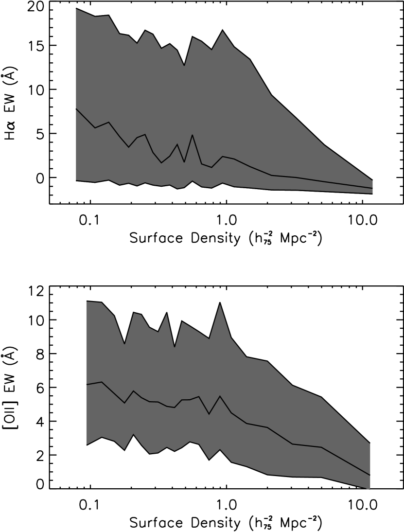
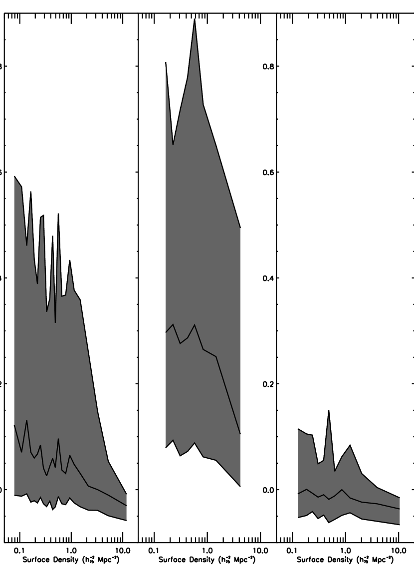
In Figure 3, we present the H and [Oii] EW distributions, as quantified by the median, the 25th, and the 75th percentiles, as a function of local density as defined above. We see an overall shift of these distributions to lower values in high density regions. Furthermore, the most strongly star–forming galaxies, i.e., the tail of the distribution for H EW Å, appears to experience the largest effect. To understand this effect further, we consider the (inverse) concentration index of SDSS galaxies (Shimasaku et al., 2001). Although concentration will be sensitive to non-morphological features like the presence of nuclear star-formation, there appears to be a reasonable correlation between and the Hubble morphological classifications as shown in Figure 10 of Shimasaku et al. (2001). For the analysis in this paper, we have chosen a threshold of to define late–type galaxies, instead of as proposed by Shimasaku et al. (2001), as our choice provides a cleaner, but more incomplete, sample of such galaxies. We estimate from Figure 10 of Shimasaku et al. (2001) that our higher threshold ensures less than 5% contamination from early–type galaxies in the late–type sample. We find that the tail of the H EW distribution is dominated by late–type (spiral) galaxies regardless of local density, i.e., % of all galaxies with H EW Å are consistent with being late–type galaxies.
We note here that the percentiles of the H and [Oii] lines appear to follow different slopes with density, with the H percentile showing almost no change with density. This is because the H EWs at Å are dominated by stellar absorption, and the strength of the absorption is only weakly dependent on the stellar population for galaxies older than a few Gyr. On the other hand, the [Oii] EW is unaffected by absorption and thus clearly shows the continual decline of emission flux into the densest regions.
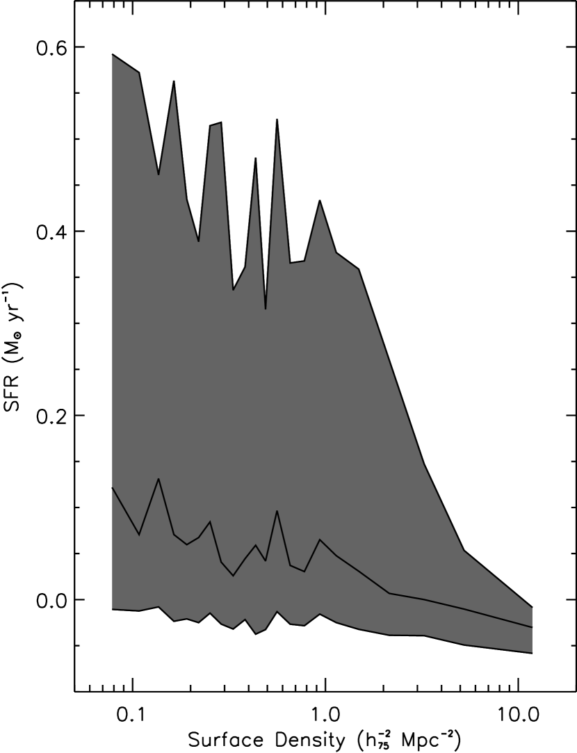
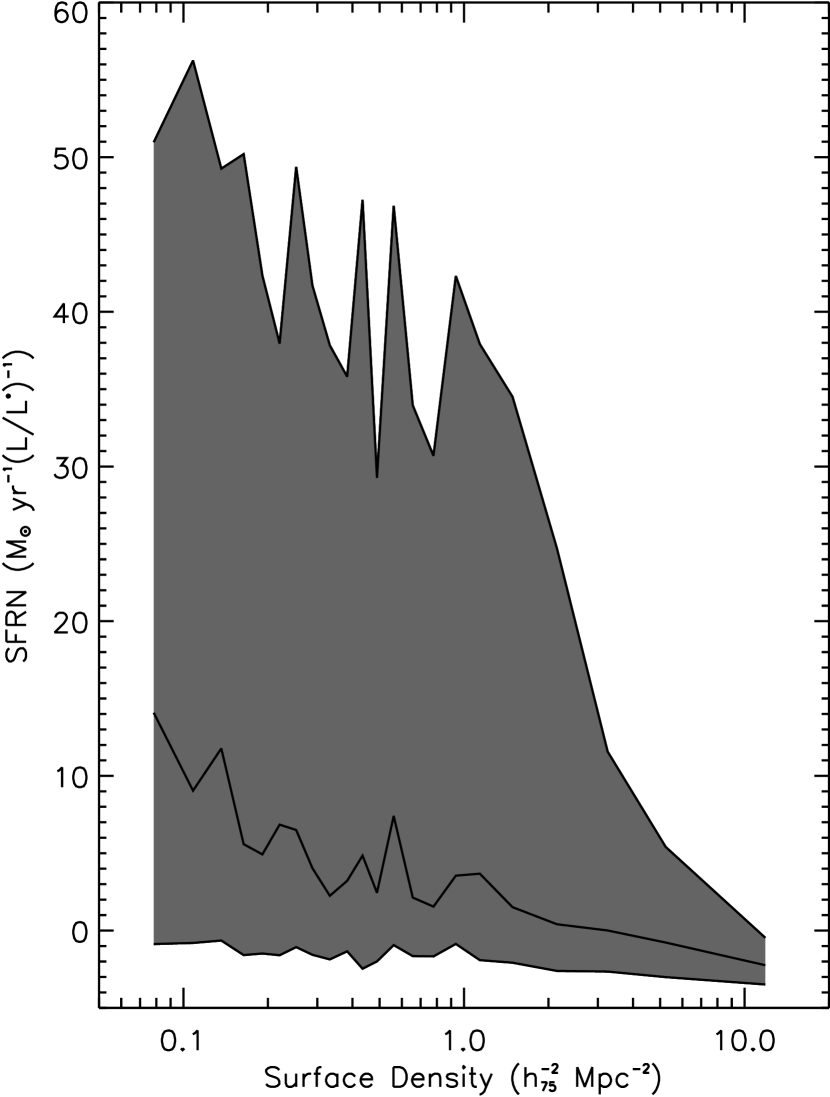
In Figure 4, we show the density–SFR relation for galaxies that is analogous to the density–morphology relation of Dressler (1980) (although the density parameters are not directly comparable). For this analysis, we have also removed obvious Active Galactic Nucleii (AGN) using the prescription outlined in Kewley et al. (2001) and using the [Nii], [Oiii], H and emission lines. If the detection of an AGN was ambiguous, based on the prescription of Kewley et al. (2001), then we do not exclude the galaxy from Figure 4. We also show the SFRN of galaxies as a function of local galaxy density, which shows two interesting phenomena: First, when compared to the corrected SFR, there is a much larger difference between the low and high density regions. This is likely an effect of the lower luminosity galaxies in the field having a higher rate of SFR per unit stellar luminosity than the more luminous galaxies. Secondly, the “break”, or characteristic density, seen in the density–SFR relation at a galaxy surface density of is much more prominent. At densities lower than this “break”, the SFR of galaxies continues to increase, i.e., in Figure 4, the median and 75th percentile of the SFRN distribution keeps increasing all the way to the lowest densities studied in this paper ().
3.2 SFR as a Function of Clustercentric Radius
We now turn our attention to virialized systems like clusters and groups of galaxies, and investigate the SFR of galaxies as a function of clustercentric radius. We test whether the features observed in the density–SFR relation, (e.g., the break or characteristic density at ) are also present in the radius–SFR relation around known virialized systems. The details of how we objectively select clusters and groups from the SDSS EDR data are in the Appendix. We also discuss the clusters and groups used in this paper in the Appendix.
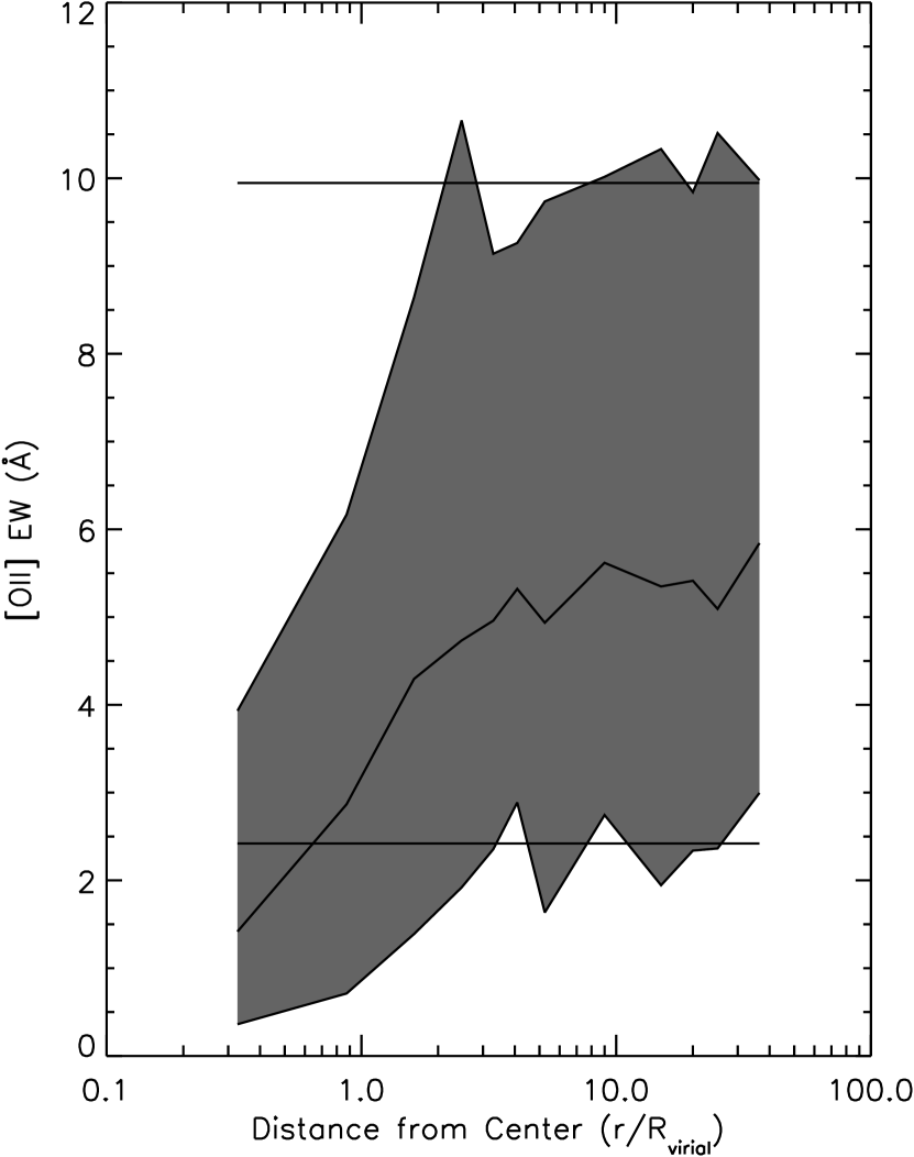
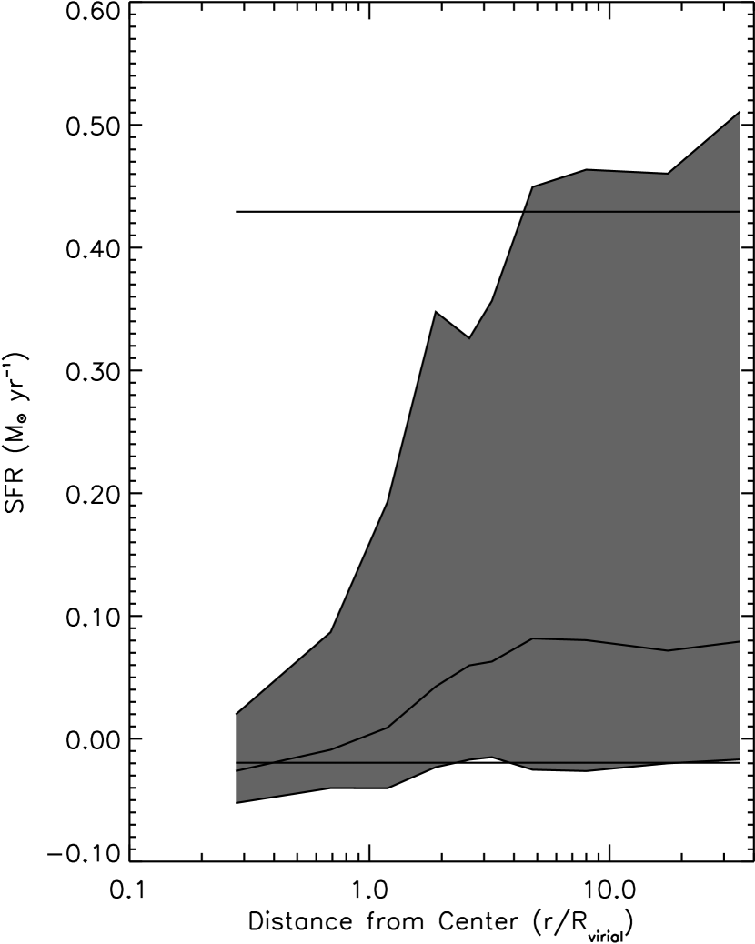
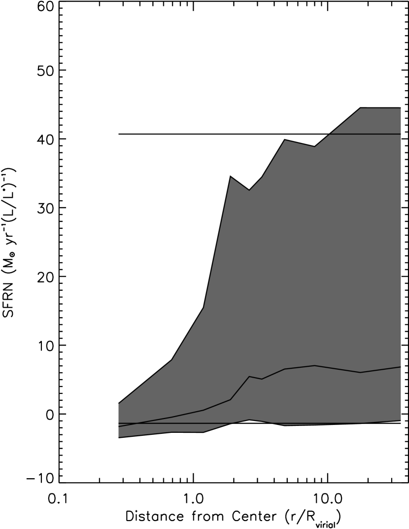
In Figure 5, we present the observed distribution of H and [Oii] EW, as quantified by the median, 25th, and 75th percentiles, as a function of (projected) clustercentric radius for groups and clusters of galaxies detected in the EDR data (see Appendix). To accommodate the wide range of masses spanned by our cluster sample, we have re–scaled all radial distances by the virial radius () of each cluster. is computed from the line–of–sight velocity dispersion, in units of km s-1, using the formula Mpc from Girardi et al. (1998). For this calculation, we used as discussed in the Appendix. For consistency with the higher redshift work, we provide measurements for both the [Oii] and H emission lines. In Figure 6, we show the same as in Figure 5, but now for the SFR and SFRN of galaxies as a function of (projected) clustercentric radius.
For comparison, we have also constructed a “non–cluster” (or field) sample of galaxies that consists of all galaxies within our volume–limited sample that are located, in redshift space, within of a cluster but are at a (projected) clustercentric distance of from any of our clusters. This methodology guards against potential redshift selection effects and/or redshift evolution of the field population, because we have defined our field population in the same redshift shells as the cluster galaxies. We note however that the difference in the mean (or median) SFR of galaxies of the field population as defined using our method and that of taking all galaxies regardless of the presence of clusters, is less than 10% (with our mean SFR measurement being systematically higher as expected). Our derived field values for the 25th and 75th percentiles are shown as lines on Figures 5 and 6.
Figures 5 and 6 show a clear decrease in the star–formation activity (in either the SFR or the EW of H and [Oii]) as a function of clustercentric radius. As seen in Figures 3 and 4, the SFR of galaxies in dense regions differ from that in the field in two ways: the whole distribution of SFRs (and EWs) is shifted to lower values, and the skewness of the distributions decreases, with the tail of the distribution containing high SFR galaxies diminishing as one enters denser environments. As discussed in Section 3.1, this tail of strongly star–forming galaxies (H EW Å) is dominated by late–type galaxies. For comparison with higher redshift studies, the mean (median) of the H and [Oii] EW distributions within one virial radius of the clusters studied herein are 3.4Å (Å) and 3.2Å (1.8Å), respectively.
The results in Figures 5 and 6 are qualitatively similar to those for distant () clusters of galaxies (Balogh et al., 1997). A new aspect of our study, however, is that we can map this decrease in SFR all the way from the cluster cores into the field population. We have used the Kolmogorov-Smirnov (KS) statistic to test the distributions of EWs and SFRs, in each radial bin of Figures 5 and 6, against the distribution of EWs and SFRs derived from our field population. This test is designed to look for global differences between two distributions and allows us to determine the clustercentric radius at which the difference between the two distributions becomes statistically significant. The distribution of H EWs becomes different from the field at the 68% () level at , while for [Oii] the distributions become different at . For SFR and SFRN, the effect of the cluster environment becomes noticeable, at the level, at clustercentric radii of and , respectively.
It is evident from Figures 5 and 6 that the tails of these distributions are more strongly environment-dependent than the medians. Therefore, we have performed a separate statistical test on the tails of the distribution and how they change with clustercentric radius. We calculated the difference between the 25th and 75th percentiles in each radial bin of Figures 5 and 6, and the corresponding 25th and 75th percentiles for the field (shown as solid, straight lines in Figures 5 and 6.) In order to assess the statistical significance of these differences, we created, for each radial bin, 1000 fake datasets via bootstrap re–sampling (with replacement) and computed, for each dataset, the same difference between cluster and field for both the 25th and 75th percentiles. This exercise provides a distribution of differences (between the cluster and field) for each radial bin for both the 25th and 75th percentiles. We then determined the probability that the observed percentile difference is consistent with zero, i.e., we just count the fraction of percentile differences above zero in these fake datasets. Using this methodology, we determined, at a greater than 68% confidence (), that the 75th (25th) percentile of the H EW distribution becomes statistically different from the field population at a clustercentric radius of (). For the SFR distribution, the 75th (25th) percentile becomes statistically different from the field population at a clustercentric radius of (). For the SFRN, the 75th (25th) percentile becomes statistically different at a clustercentric radius of ()
These tests demonstrate that the SFR distribution of the galaxy population differs from the field (at ) out to virial radii. These radii correspond to Mpc, based on the average virial radii computed for the clusters given in Table 1. These tests confirm that all levels of SFR are affected, with the most strongly star–forming galaxies being affected more severely (i.e., the 75th percentile) than the quiescent population. The implications of these results will be discussed in Section 4.
To fully understand the correspondence between the radius–SFR relation and the density–SFR relation presented in Section 3.1, we present the correlation between the local projected density and clustercentric radius measured for each galaxy within the vicinity of our 17 clusters and groups. As expected, there is a linear correlation between these two quantities, and the characteristic density of in Figure 4 corresponds to a range of clustercentric radii from to virial radii. This range of radii is consistent with our observations above in that the distribution of SFRs in cluster galaxies begin to differ from the field population at to virial radii.
4 Discussion
4.1 Possible Biases and Systematic Errors
Before we interpret our results, we must first investigate the effects of possible systematic biases on our work. These include the effect of: i) The SDSS analysis software and the SDSS survey observing strategy; ii) Aperture bias due to the 3 arcsecond fiber width; iii) Reddening due to dust in the host galaxies; and iv) The smearing correction performed by the SDSS to improve the flux calibration of the continuum. We present a detailed analysis of these possible biases in the Appendix, but we find that none of these potential biases have a large effect on our results.
4.2 The Density–Morphology Relation
As we move towards denser environments, the galaxy population becomes dominated by early-type galaxies that have a lower intrinsic SFR (Kennicutt, 1983; Jansen et al., 2000). In this section, we attempt to determine whether or not the SFR of galaxies of a given morphology are themselves affected by environment, i.e., is the density–SFR relation distinct from the density–morphology relation? Previously, Balogh et al. (1998) have attempted to answer this question using an objective morphological classification, based on a galaxy bulge-to-disk luminosity, that was then correlated with the radial dependence of SFR in distant clusters. They concluded that cluster galaxies of a given redshift, luminosity, and bulge-to-disk ratio had lower star formation rates compared with their counterparts in the field. Some evidence supporting this has also been reported by Hashimoto et al. (1998), Couch et al. (2001), Balogh et al. (2002a) and Pimbblet et al. (2001). We have attempted to address this issue in this paper in two different ways. First, using a subset of SDSS galaxies that possess both a visual morphological classification (from either Dressler 1980 or Shimasaku et al. 2001) and a SDSS H EW measurement. Secondly, using objective morphologies based on the (inverse) concentration index of SDSS galaxies as discussed in Section 3.1. We discuss these two tests below.
We have cross–correlated our sample of galaxies with samples of Dressler (1980) and Shimasaku et al. (2001). For the Dressler (1980) cluster sample, we find 114 galaxies in common with our sample and thus have a SDSS H measurement. The sample includes ellipticals, spirals and lenticulars that satisfy our selection criteria (Section 2.2). For the Shimasaku et al. (2001) sample, which provides morphological classifications for 456 SDSS galaxies, selected over a representative range of environments, we find 57 early–type galaxies and 73 late–type galaxies that satisfy our selection criteria (outlined in Section 2.2). In this case, we have added together the ellipticals and lenticulars because of the concerns noted by Shimasaku et al. (2001) regarding their tendency to preferentially classify lenticular as ellipticals, compared with the RC3 catalog. Overall, these two samples of morphologically–classified galaxies cover a similar range in luminosity and redshift as the galaxy sample outlined in Section 2.2. The largest systematic uncertainty is in the consistency between the morphological classifications.
In Figure 8, we show the distribution of H EWs for these galaxy samples as a function of their morphological type. We see a difference (confirmed using a KS test) in the H EW distribution of spirals between these two samples, i.e., the Dressler sample of spirals has, on average, a lower SFR than seen in the Shimasaku et al. (2001) sample. This difference could be due to one or more of the following possibilities. First, it could reflect a real environment effect, that cluster spirals have lower SFR than the average field spiral population. Second, it could be due to the fact that the morphological bins are too coarse to define a homogeneous galaxy population. A different relative distribution of Sa and Sc galaxies in the two samples, for example, could give rise to the same trend (see Shane & James, 2001). Third, the difference may reflect inconsistencies in the morphological classification criteria in the two samples. Thus, although these results are intriguing, a more definitive answer will require an automated classification of the SDSS galaxy morphologies, on a continuous scale.
As a first attempt of this, we have used the (inverse) concentration index discussed in Section 3.1 to investigate the degeneracy between the density–morphology and the density–SFR relations. This galaxy parameter can be used as an objective morphological classification, but is hard to interpret and to compare directly to the visual morphologies. In Figure 9, we present the distribution of SFRN as a function of projected local galaxy density (as originally presented in Figure 4), but split the sample into two broad morphological bins based on the (inverse) concentration index, i.e., late–type galaxies (with , see Section 3.1) and early–type galaxies (with ). As discussed in Section 3.1, the tail of the SFR distribution (with high H EWs) is dominated by late–type galaxies at all densities. This plot also demonstrates that the late–type galaxies in our sample lie on a density–SFR relation similar to the one observed for the whole sample. As expected, the early–type galaxies have little, or no, star–formation, but they also appear to follow a shallow density–SFR relation (for this sample however, we must be concerned about contamination from the late–type galaxies and the effects of stellar absorption).
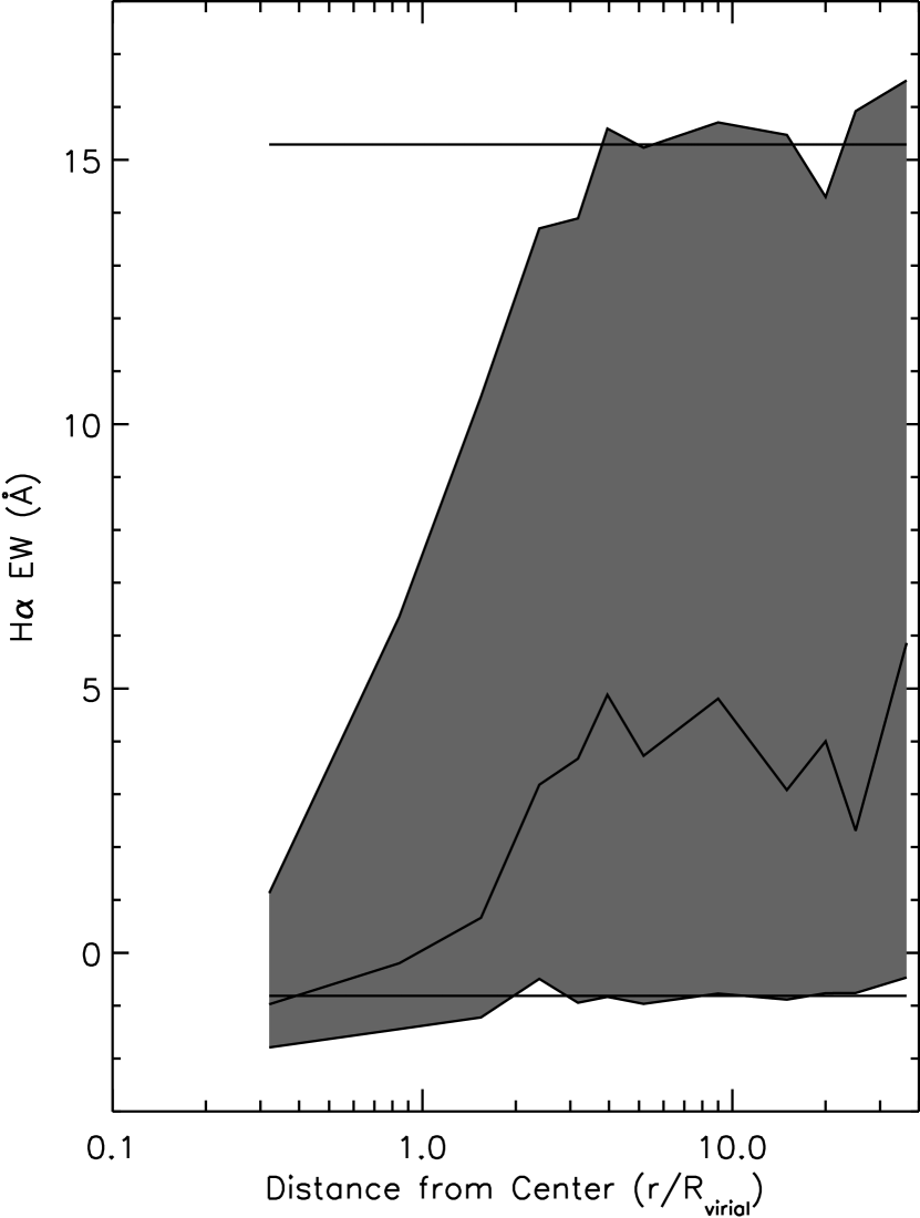
To quantify these effects in more detail, we present in Figure 10, the distribution of H EW as a function of clustercentric radius for all galaxies as well as just the late–type galaxies (with ). We have performed a KS test between the late–type galaxies () in the tails (Å) of the four H EW distributions in Figure 10 (the black filled histograms) and the late–type galaxies in the field (i.e., also with and Å). This analysis indicates that the inner three clustercentric radii (, , ) are inconsistent with the field population, at the 82.5%, 71% and 99.8% probability levels, respectively. This suggests that the distribution of H EWs for strongly star–forming (Å) late–type galaxies does change with density, which is consistent with our results in Section 3.1 and with those of Hashimoto et al. (1998).
4.3 Physical Interpretation
The most striking result of this paper is the critical density (or radius) where the SFR of galaxies changes from that of the field. This happens at a density of , which corresponds to a clustercentric distance of between and virial radii. In this section, we attempt to understand this observation within the context of hierarchical structure formation. In hierarchical models, clusters and groups form from slightly overdense regions in the initial matter distribution. At first, clusters expand with the Hubble flow until they reach a maximum size and then de–couple from the expansion and collapse to form a virialized object. Using the spherical collapse model (Gunn & Gott, 1972), one can show that the point of maximal size, also called the “turn–around” radius (), is equal to a density of approximately six times the mean density of the background at that time. The virial radius () corresponds to a radius where the density is a few hundred times the mean density of the background. Therefore, there are two natural scales for an overdensity in the Universe – the virial radius and the turn–around radius – and the latter radius marks the limit of the gravitational influence of a cluster or group. The region between the two scales is known as the infall region.
We can estimate the ratio of virial () and turn–around () radius as follows. Suppose that the region between and is completely empty. Then , where and are the masses of the cluster within the turn–around and virial radii, respectively. Using and , we find . In practice however, the region between and is not empty and a more realistic case is to assume that clusters or groups of galaxies follow, for example, the NFW mass density profile (Navarro et al., 1996). We can thus find the turn–around radius by integrating the profile until . In this case, we find that , which is in good agreement with our naive calculation above.
It is intriguing that this scale () is comparable to the scale at which the cluster SFR becomes statistically indistinguishable from the field. However, it is unclear that this radius has any physical meaning that might effect the SFR of individual galaxies, as the mechanisms proposed for changing the SFR of galaxies in the cores of rich clusters, e.g., ram-pressure stripping of the gas, galaxy harassment (Moore et al., 1999), tidal disruption (Byrd & Valtonen, 1990), are unlikely to be important at low densities and/or large virial radii. A more appropriate mechanism for changing the SFR of these galaxies may be the merger or close tidal interactions of galaxies in less dense groups within the infall regions of clusters (Zabludoff et al., 1996; Zabludoff & Mulchaey, 1998; Kodama et al., 2001).
To obtain a more detailed physical understanding of our results, we must compare our observations with numerical simulations. For example, Balogh et al. (2000) and Diaferio et al. (2001) have recently showed that simple (heuristic) models for the gas depletion of galaxies within hierarchical models of structure formation are able to accurately reproduce the decrease in the star–formation rate of galaxies seen within the cores of CNOC1 clusters of galaxies (Balogh et al., 1997, 1998). In both these works, the SFR of a galaxy is affected by both local and external processes. Locally, the SFR is governed solely by the consumption rate of cold gas in the disk, dependent only on gas density and the feedback model. The only external process that effects the SFR of a single galaxy is the stripping of its hot gas reservoir after it merges with a larger (e.g., group or cluster) halo. Following this, the SFR declines gradually, as the galaxy consumes the remaining cold, disk gas. Therefore, the main physical properties of a galaxy in the simulation that controls these processes are the amount of cool gas in the galaxy and the time since the last interaction with a larger halo. Diaferio et al. (2001) predicts that the mean SFR of galaxies in clusters should be lower than the field out to (here is a 3–dimensional radius from the simulations, while throughout the paper, we have quoted as a projected radius from the cluster cores). This reduction is due to galaxies that had been near the cluster core, but thrown out to large radii during major mergers (Balogh et al., 2000; Evrard & Gioia, 2002). Our results are qualitatively similar to the predictions of Balogh et al. (2000) and Diaferio et al. (2001) in that these hierarchical models of structure formation can affect the SFR of galaxies beyond the virial radius. However, we will require further comparison of the simulations and observations to determine if these simple models are all that is required to explain the data, or whether we need additional physical processes that effect the SFR of galaxies at larger radii in the infall regions of clusters, i.e., from 2 to 4.
4.4 Comparison with Previous Work
A similar analysis has been carried out using the LCRS (Hashimoto et al., 1998) and 2dF Galaxy Redshift Survey (2dFGRS) data (Lewis et al., 2002). For the 2dFGRS, the luminosity limits, redshift limits, and H EW distributions are comparable with our sample, and both studies are remarkably consistent in their main conclusions. First, star formation is reduced, relative to the field, out to virial radii from known clusters and groups. Secondly, there appears to be a critical density of galaxy (brighter than ) per Mpc2, below which there is a weaker correlation with star-formation rate.
Our work moves beyond the 2dF study in several ways. Most importantly, we have computed a local density for every galaxy in the EDR, regardless of its proximity to a cluster. Moreover, our cluster catalog is dominated by systems with much lower velocity dispersions than those in Lewis et al. (2002), so it further emphasizes that the density–SFR relation is universal and does not depend on the large-scale mass of the embedding structure. Furthermore, Lewis et al. (2002) are unable to compute H fluxes, and hence star formation rates, due to uncertainty in the continuum fluxing. This is not a problem for the SDSS, and we have been able to show that there exists an absolute density–SFR relation, as well as a relative one. We have also used the fluxes from another line ([Oii]) to demonstrate that our results are robust to the effects of reddening. Finally, the data analysed by Lewis et al. (2002) are preliminary in the sense that sampling is not complete over their full extracted regions. The consistency between our results shows that this is not a large problem.
Recently, Kodama et al. (2001) reported the detection of a “break” in the colors of galaxies around distant cluster Abell 851 (). They observed an abrupt change in the colors of galaxies at a local surface density of galaxies of , which corresponds to a radial distance of from the center of this cluster. Even after correcting for the differences in the luminosity limits of the two data sets ( in Kodama et al. (2001) compared to here), the “break” seen by Kodama et al. (2001) occurs at an order of magnitude greater surface density, and also a smaller clustercentric radius, than the “break” reported here. Further observations will be needed to determine if this difference is physical (i.e., due to differences in the redshift or luminosity limits of the two studies) or an artifact of the different analyses.
4.5 Future Work
As the SDSS database increases, we will be able to increase the size and depth of the sample used herein, i.e., to increase the number of galaxy clusters, as well as to relax some of the conservative selection criteria we have imposed on our present sample. Furthermore, we will use additional information on these galaxies extracted from both the SDSS photometry and spectra. For example, we can use the five passband SDSS photometry to look for color gradients within these galaxies to fully correct for the aperture biases as well as study how the environment effects the star formation within a galaxy (see Moss & Whittle, 1993, 2000; Rose et al., 2001). We must also extend our study to characterize the effects of the environment on the overall star formation history of galaxies. For instance, we should include post–starburst galaxies (E+A, k+a and a+k; see Zabludoff et al., 1996; Poggianti et al., 1999; Balogh et al., 1999; Castander et al., 2001), because these may be key to fully understanding star–formation activity within dense environments. In addition, we should probe fainter luminosities to determine the rate of change of SFR per unit stellar luminosity.
Most importantly, the research discussed in Section 4.2 clearly requires a more robust, automated morphology for each of the SDSS galaxies similar to the bulge–to–disk decompositions used by others (Balogh et al., 1998, 2002b). We can then perform a multi–variate analysis on the galaxy population that treats the SFR, local density, morphology, mass and luminosity of the galaxies in a self–consistent manner. We must also expand our definition of local density to include more information on the higher–order moments of the galaxy distribution, e.g., filaments. A full characterization of the effect of the environment on the overall star formation history of galaxies is paramount to our understanding of the physical processes that could be responsible for galaxy evolution.
5 Conclusions
We have investigated the effects of the local galaxy environment on the star–formation of galaxies using the Early Data Release of the Sloan Digital Sky Survey. For this work, we have restricted our analysis to a volume–limited sample of 8598 galaxies brighter than (k–corrected, for ) over the redshift range . For all galaxies, we have characterized the star–formation using the H and [Oii] EWs, as well as by computing their star–formation rates (SFR) and normalized star–formation rates (SFRN; SFR per unit luminosity) from the SDSS data. We have quantified the local galaxy environment using the projected distance to the 10th nearest neighbor brighter than as well as by measuring the clustercentric distance of galaxies from the cores of known clusters and groups of galaxies (see Appendix). We have extensively tested our results as discussed in detail in the Appendix.
This work expands upon previous studies of the SFR of galaxies as a function of environment in four ways: i) We extend such studies into the group and poor cluster regime; ii) We focus on the low redshift universe; iii) We have traced the SFR activity of galaxies well beyond the cores of the clusters and groups into the field population; and iv) We are able to accurately quantify the local galaxy density in a uniform manner that is not subject to statistical background correction. We conclude that:
-
•
The distributions of [Oii] and H EWs, as quantified by the median and 25th and 75th percentiles, changes as a function of local galaxy density as measured using the distance to the nearest neighbor. We witness similar relations in the SFR and SFRN of galaxies as shown in Figure 4. This effect is characterized in three ways. First, there is shift in the overall distributions of EW, SFR, and SFRN to lower values with increasing galaxy density. Secondly, the skewness of the distributions decreases with increasing local galaxy density, i.e., the tail of strongly star–forming galaxies (H EW Å), as quantified by the 75th percentile of the distribution, is noticeably decreased in high density regions. Finally, we see a “break” (or characteristic scale) in the correlation between SFR (and SFRN) and density at a local galaxy density of (for galaxies brighter than ). Figures 3 and 4 represent the density–SFR relation of galaxies that is analogous to the density–morphology relation of galaxies (Dressler 1980).
-
•
The distribution of EW, SFR, and SFRN of galaxies, as quantified by the median and 25th and 75th percentiles, changes as a function of clustercentric radius for the clusters and groups discussed in this paper (see Table 1). This effect is most noticeable for the strongly star–forming galaxies in the 75th percentiles of the distribution. Using a KS test and boot–strapping re-sampling techniques, we find that the star formation rates of galaxies begin to decrease, compared with field galaxies, starting at 3-4 virial radii (with statistical significance). Within one virial radius of our clusters, the means (medians) of the H and [Oii] EW distributions are 3.4Å (Å) and 3.2Å (1.8Å), respectively.
-
•
As shown in Figure 7, the break or characteristic density seen at a (projected) galaxy density of Mpc in the density–SFR relation corresponds to and virial radii for the systems discussed in this paper. Therefore, there is good agreement between our results from the clusters and groups (discussed in Section 3.2) and the general density–SFR relation (discussed in Section 3.1).
-
•
We have investigated the possible degeneracy between our density–SFR relation and the density–morphology relation (Dressler 1980). There is some evidence that the SFR of galaxies in dense regions varies even among galaxies of the same morphology. For example, we have used the (inverse) concentration index of SDSS galaxies to show that the tail of the strongly star–forming (H EW Å) galaxies observed in the H EW, SFR, and SFRN distributions is dominated (%) by late–type (spiral) galaxies. Using a KS test, we have shown that this tail of late–type galaxies is different in dense regions (within 2 virial radii) compared with similar galaxies in the field. We stress, however, that the significance of these results remains uncertain at present due to potential systematic biases in the morphological classifications used herein.
-
•
Our results are qualitatively consistent with the predictions of Balogh et al. (2000) and Diaferio et al. (2001) in that these hierarchical models of structure formation can affect the SFR of galaxies well beyond the virial radius. However, we require more detailed comparisons between the simulations and observations to determine if such simple (heuristic) models are all that is necessary to explain the data, or whether we need additional processes that affect the SFR of galaxies at large clustercentric radii and/or low densities.
-
•
Our results are in good agreement with the recent 2dF work of Lewis et al. (2002) as well as consistent with previous observations of a decrease in the SFR of galaxies in the cores of distant clusters (Balogh et al. 1997; 1998). Taken together, these results demonstrate that the decrease in SFR of galaxies in dense environments is a universal phenomenon over a wide range in densities (from the rarefied field to poor groups to rich clusters) and redshifts.
References
- Abell, Corwin, & Olowin (1989) Abell, G. O., Corwin, H. G., & Olowin, R. P. 1989, ApJS, 70, 1.
- Böhringer et al. (2001) Böhringer, H., Schuecker, P., Guzzo, L., Collins, C. A., Voges, W., Schindler, S., Neumann, D. M., Cruddace, R. G., De Grandi, S., Chincarini, G., Edge, A. C., MacGillivray, H. T., & Shaver, P. 2001, A&A, 369, 826
- Balogh et al. (1997) Balogh, M. L., Morris, S. L., Yee, H. K. C., Carlberg, R. G., & Ellingson, E. 1997, ApJL, 488, 75
- Balogh et al. (1999) —. 1999, ApJ, 527, 54
- Balogh et al. (1998) Balogh, M. L., Schade, D., Morris, S. L., Yee, H. K. C., Carlberg, R. G., & Ellingson, E. 1998, ApJL, 504, 75
- Balogh et al. (2000) Balogh, M. L., Navarro, J. F., & Morris, S. L. 2000, ApJ, 540, 113
- Balogh et al. (2002a) Balogh, M. L., Couch, W. J., Smail, I., Bower, R. G., & Glazebrook. 2002a, MNRAS, submitted
- Balogh et al. (2002b) Balogh, M. L., Smail, I., Bower, R. G., Ziegler, B. L., Smith, G. P., Davies, R. L., Gaztelu, A., Kneib, J.-P., & Ebeling, H. 2002b, ApJ, 566, 123
- Bartholomew et al. (2001) Bartholomew, L. J., Rose, J. A., Gaba, A. E., & Caldwell, N. 2001, AJ, 122, 2913
- Baugh et al. (1996) Baugh, C. M., Cole, S., & Frenk, C. S. 1996, MNRAS, 283, 1361
- Bekki et al. (2002) Bekki, K., Shioya, Y., Couch, W. J., 2002, ApJ, accepted (astro-ph/0206207)
- Bernstein et al. (1995) Bernstein, G. M., Nichol, R. C., Tyson, J. A., Ulmer, M. P., & Wittman, D. 1995, AJ, 110, 1507
- Blanton et al. (2001) Blanton, M. R., Dalcanton, J., Eisenstein, D., Loveday, J., Strauss, M. A., SubbaRao, M., Weinberg, D. H., & the Sloan collaboration. 2001, AJ, 121, 2358
- Byrd & Valtonen (1990) Byrd, G. & Valtonen, M. 1990, ApJ, 350, 89
- Castander et al. (2001) Castander, F. J., Nichol, R. C., Merrelli, A., Burles, S., Pope, A., Connolly, A. J., Uomoto, A., Gunn, J. E., Anderson, J. E., Annis, J., Bahcall, N. A., Boroski, W. N., Brinkmann, J., Carey, L., Crocker, J. H., Csabai, I. ., Doi, M., Frieman, J. A., Fukugita, M., Friedman, S. D., Hilton, E. J., Hindsley, R. B., Ivezić, Ž., Kent, S., Lamb, D. Q., Leger, R. F., Long, D. C., Loveday, J., Lupton, R. H., MacGillivray, H., Meiksin, A., Munn, J. A., Newcomb, M., Okamura, S., Owen, R., Pier, J. R., Rockosi, C. M., Schlegel, D. J., Schneider, D. P., Seigmund, W., Smee, S., Snir, Y., Starkman, L., Stoughton, C., Szokoly, G. P., Stubbs, C., SubbaRao, M., Szalay, A., Thakar, A. R., Tremonti, C., Waddell, P., Yanny, B., & York, D. G. 2001, AJ, 121, 2331
- Charlot et al. (2001) Charlot, S. ., Kauffmann, G., Longhetti, M., Tresse, L., White, S. D. M., Maddox, S. J., & Fall, S. M. 2001, MNRAS, in press, astroph/111289
- Charlot & Longhetti (2001) Charlot, S. . & Longhetti, M. 2001, MNRAS, 323, 887
- Cole et al. (2000) Cole, S., Lacey, C. G., Baugh, C. M., & Frenk, C. S. 2000, MNRAS, 319, 168
- Couch et al. (2001) Couch, W. J., Balogh, M. L., Bower, R. G., Smail, I., Glazebrook, K., & Taylor, M. 2001, ApJ, 549, 820
- Diaferio et al. (2001) Diaferio, A., Kauffmann, G., Balogh, M. L., White, S. D. M., Schade, D., & Ellingson, E. 2001, MNRAS, 323, 999
- Dressler (1980) Dressler, A. 1980, ApJ, 236, 351
- Dressler et al. (1997) Dressler, A., Oemler, A., Couch, W. J., Smail, I., Ellis, R. S., Barger, A., Butcher, H. R., Poggianti, B. M., & Sharples, R. M. 1997, ApJ, 490, 577
- Evrard & Gioia (2002) Evrard, A. E. & Gioia, I. 2002, ApJ, in preparation
- Fukugita et al. (1996) Fukugita, M., Ichikawa, T., Gunn, J. E., Doi, M., Shimasaku, K., & Schneider, D. P. 1996, AJ, 111, 1748
- Girardi et al. (1998) Girardi, M., Giuricin, G., Mardirossian, F., Mezzetti, M., & Boschin, W. 1998, ApJ, 505, 74
- Gladders & Yee (2000) Gladders, M. D. & Yee, H. K. C. 2000, AJ, 120, 2148
- Goto et al. (2002) Goto, T., Sekiguchi, M., Nichol, R. C., Bahcall, N. A., Kim, R. S. J., Annis, J., Ivezic, Z., Brinkmann, J., Hennessy, G. S., Szokoly, G. P., & Tucker, D. L. 2002, AJ, in press, astroph/0112482
- Gunn & Gott (1972) Gunn, J. E. & Gott, J. R. I. 1972, ApJ, 176, 1
- Gunn et al. (1998) Gunn, J. E. et al. 1998, AJ, 116, 3040
- Hashimoto et al. (1998) Hashimoto, Y., Oemler, A. J., Lin, H., & Tucker, D. L. 1998, ApJ, 499, 589
- Heavens (1993) Heavens, A. F. 1993, MNRAS, 263, 735
- Hopkins et al. (2001) Hopkins, A. M., Connolly, A. J., Haarsma, D. B., & Cram, L. E. 2001, AJ, 122, 288
- Hogg et al. (1998) Hogg, D. W., Schlegel, D. J., Finkbeiner, D. P., & Gunn, J. E. 2001, AJ, 122, 2129
- Jansen et al. (2000) Jansen, R. A., Fabricant, D., Franx, M., & Caldwell, N. 2000, ApJS, 126, 331
- Kauffmann et al. (1993) Kauffmann, G., White, S. D. M., & Guiderdoni, B. 1993, MNRAS, 264, 201
- Kennicutt (1983) Kennicutt, R. C. 1983, ApJ, 272, 54
- Kennicutt (1992) —. 1992, ApJ, 388, 310
- Kennicutt (1998a) Kennicutt, R. C., J. 1998a, ARA&A, 36, 189
- Kennicutt (1998b) Kennicutt, R. C. 1998b, ApJ, 498, 541
- Kewley et al. (2001) Kewley, L. J., Dopita, M. A., Sutherland, R. S., Heisler, C. A., & Trevena, J. 2001, ApJ, 556, 121
- Konchanek et al (2000) Kochanek, C.S., Pahre, M.A., Falco, E.E., 2000, submitted, see astro-ph/0011458
- Kodama et al. (2001) Kodama, T., Smail, I., Nakata, F., Okamura, S., & Bower, R. G. 2001, ApJL, 562, L9
- Lewis et al. (2002) Lewis, I., Balogh, M., De Propris, R., Couch, W., Bower, R., Offer, A., Bland-HAwthorn, J., Baldry, I. K., Baugh, C., Bridges, T., Cannon, R., Cole, S., Colless, M., Collins, C., Cross, N., Dalton, G., P., D. S., Efstathiou, G., Ellis, R. S., Frenk, C. S., Glazebrook, K., Hawkins, E., Jackson, C., Lahav, O., Lumsden, S., Maddox, S., Madgwick, D., Norberg, P., Peacock, J. A., Percival, W., Peterson, B. A., Sutherland, W., & Taylor, K. 2002, MNRAS, in press
- Lilly et al. (1996) Lilly, S. J., Le Fevre, O., Hammer, F., & Crampton, D. 1996, ApJL, 460, L1
- Lupton et al. (2001) Lupton, R. H., Gunn, J. E., Ivezić, Z., Knapp, G. R., Kent, S., & Yasuda, N. 2001, in Astronomical Data Analysis Software and Systems X, ASP Conference Proceedings, Vol. 238. Edited by F. R. Harnden, Jr., Francis A. Primini, and Harry E. Payne. San Francisco: Astronomical Society of the Pacific, ISSN: 1080-7926, 2001., p.269, Vol. 10, 269
- Lupton et al. (1999) Lupton, R. H., Gunn, J. E., & Szalay, A. S. 1999, AJ, 118, 1406
- Magliocchetti et al. (2000) Magliocchetti, M., Maddox, S. J., Wall, J. V., Benn, C. R., & Cotter, G. 2000, MNRAS, 318, 1047
- Mahdavi & Geller (2001) Mahdavi, A. & Geller, M. J. 2001, ApJL, 554, L129
- Miller et al. (2001) Miller, C. J., Genovese, C., Nichol, R. C., Wasserman, L., Connolly, A., Reichart, D., Hopkins, A., Schneider, J., & Moore, A. 2001, AJ, 122, 3492
- Moore et al. (1999) Moore, B., Lake, G., Quinn, T., & Stadel, J. 1999, MNRAS, 304, 465
- Moss & Whittle (1993) Moss, C. & Whittle, M. 1993, ApJL, 407, L17
- Moss & Whittle (2000) —. 2000, MNRAS, 317, 667
- Navarro et al. (1996) Navarro, J. F., Frenk, C. S., & White, S. D. M. 1996, ApJ, 462, 563
- Nichol et al. (2001) Nichol, R. C. et al. 2001, Mining the Sky, 613.
- Pier et al. (2002) Pier, J. R., Munn, J. A., Hindsley, R. B., Hennessy, G. S., Kent, S. M., Lupton, R. H., & Ivezic, Z. 2002, AJ, submitted
- Pimbblet et al. (2001) Pimbblet, K. A., Smail, I., Kodama, T., Couch, W. J., Edge, A. C., Zabludoff, A. I., & O’Hely, E. 2001, MNRAS, in press
- Poggianti et al. (1999) Poggianti, B. M., Smail, I., Dressler, A., Couch, W. J., Barger, A. J., Butcher, H., Ellis, R. S., & Oemler, A. 1999, ApJ, 518, 576
- Postman & Geller (1984) Postman, M. & Geller, M. J. 1984, ApJ, 281, 95
- Postman et al. (2001) Postman, M., Lubin, L. M., & Oke, J. B. 2001, AJ, 122, 1125
- Quilis et al. (2000) Quilis, V., Moore, B., & Bower, R. 2000, Science, 288, 1617
- Rose et al. (2001) Rose, J. A., Gaba, A. E., Caldwell, N., & Chaboyer, B. 2001, AJ, 121, 793
- Salpeter (1955) Salpeter, E. E. 1955, ApJ, 121, 161
- Schlegel et al. (1998) Schlegel, D. J., Finkbeiner, D. P., & Davis, M. 1998, ApJ, 500, 525
- Shane & James (2001) Shane, N. S. & James, P. A. 2001, astro-ph/, 0112183
- Shimasaku et al. (2001) Shimasaku, K., Fukugita, M., Doi, M., Hamabe, M., Ichikawa, T., Okamura, S., Sekiguchi, M., Yasuda, N., Brinkmann, J., Csabai, I. ., Ichikawa, S., Ivezić, Z., Kunszt, P. Z., Schneider, D. P., Szokoly, G. P., Watanabe, M., & York, D. G. 2001, AJ, 122, 1238
- Smith et al. (2002) Smith, J. A. et al. 2002, AJ, 123, 2121
- Somerville & Primack (1999) Somerville, R. S. & Primack, J. R. 1999, MNRAS, 310, 1087
- Stickel et al. (2002) Stickel, M., Klaas, K., Lemke, D., & Mattila, K. 2002, A&A, 383, 367
- Stoughton et al. (2002) Stoughton, C. et al. 2002, AJ, 123, 485.
- Strauss et al. (2002) Strauss, M. et al. 2002, AJ, submitted
- Sullivan et al. (2001) Sullivan, M., Mobasher, B., Chan, B., Cram, L., Ellis, R., Treyer, M., & Hopkins, A. 2001, ApJ, 558, 72
- Voges et al. (2000) Voges, W., Aschenbach, B., Boller, T., Brauninger, H., Briel, U., Burkert, W., Dennerl, K., Englhauser, J., Gruber, R., Haberl, F., Hartner, G., Hasinger, G., Pfeffermann, E., Pietsch, W., Predehl, P., Schmitt, J., Trumper, J., & Zimmermann, U. 2000, VizieR Online Data Catalog, 9029, 0
- Whitmore et al. (1993) Whitmore, B. C., Gilmore, D. M., & Jones, C. 1993, ApJ, 407, 489
- York et al. (2000) York, D. G., Adelman, J., Anderson, J. E., Anderson, S. F., Annis, J., Bahcall, N. A., Bakken, J. A., Barkhouser, R., & the Sloan collaboration. 2000, AJ, 120, 1579
- Zabludoff et al. (1996) Zabludoff, A. I., Zaritsky, D., Lin, H., Tucker, D., Hashimoto, Y., Shectman, S. A., Oemler, A., & Kirshner, R. P. 1996, ApJ, 466, 104
- Zabludoff & Mulchaey (1998) Zabludoff, A. I. & Mulchaey, J. S. 1998, ApJ, 496, 39
- Zaritsky, Zabludoff, & Willick (1995) Zaritsky, D., Zabludoff, A. I., & Willick, J. A. 1995, AJ, 110, 1602.
Acknowledgements
We would like to thank Rupert Croft, Tim Heckman, David Schlegel, Larry Wasserman, Christy Tremonti, Guinevere Kauffmann and Daniel Eisenstein for useful discussions about this work. We thank the 2dFGRS team for sharing their results with us prior to publication. We thank an anonymous referee for his helpful comments which made this paper better. PG and AKR acknowledge financial support from the NASA LTSA program (grant number NAG5-7926). TG acknowledges financial support from the Japan Society for the Promotion of Science (JSPS) through JSPS Research Fellowships for Young Scientists. MLB acknowledges support from a PPARC rolling grant for extragalactic astronomy at Durham. AIZ acknowledges support form the NASA LTSA program (grant number NAG5-11108). Funding for the creation and distribution of the SDSS Archive has been provided by the Alfred P. Sloan Foundation, the Participating Institutions, the National Aeronautics and Space Administration, the National Science Foundation, the U.S. Department of Energy, the Japanese Monbukagakusho, and the Max Planck Society. The SDSS Web site is http://www.sdss.org/. The SDSS is managed by the Astrophysical Research Consortium (ARC) for the Participating Institutions. The Participating Institutions are The University of Chicago, Fermilab, the Institute for Advanced Study, the Japan Participation Group, The Johns Hopkins University, Los Alamos National Laboratory, the Max-Planck-Institute for Astronomy (MPIA), the Max-Planck-Institute for Astrophysics (MPA), New Mexico State University, Princeton University, the United States Naval Observatory, and the University of Washington
.1 Selection of the Groups and Clusters of Galaxies
A critical part of our study of galaxy star–formation activity in dense environments is the selection of virialized groups and clusters of galaxies within the EDR. This was achieved using the objective C4 algorithm described in Nichol et al. (2001) and Miller et al. (2002, in prep.), which assumes that galaxy groups and clusters have a co-evolving set of galaxies with similar colors, e.g., within the E/S0 ridgeline. Like any cluster–finding algorithm, this does bias our selection of systems because we assume a model for the objects that we are searching for. However, such biases can be quantified using simulations (see Miller et al. 2002, in prep.) and is preferred to using visually–compiled catalogs, like Abell (Abell, Corwin, & Olowin, 1989), whose selection function is hard to quantify through simulations. We stress that these criteria are used only to find the clusters and not to assign membership for subsequent analysis.
We briefly outline the methodology we used herein which is based on the C4 algorithm discussed in more detail in Miller et al. (2002, in prep). For each galaxy in our sample, we count the number of neighbors within a seven-dimensional box (four colors, RA, DEC and a redshift). The size of the box in the color dimensions is determined from the errors in the galaxy magnitudes and the intrinsic scatter in galaxy colors within the cores of groups and clusters. The angular size corresponds to 1 hMpc at the redshift of the galaxy. The size of the box in the redshift direction is and thus only rejects obvious foreground and background galaxies. We then compare this galaxy count (around each galaxy) to the distribution of neighbor counts for the whole field population and calculate the probability that the target galaxy is a field galaxy. The field distribution is determined by moving the seven-dimensional box to 100 randomly chosen galaxies with similar seeing and galactic extinction measurements. Using the False Discovery Rate thresholding technique of Miller et al. (2001), we then identify galaxies that have a low probability of being in the field, i.e., such that of these galaxies could be mistaken field galaxies. We note that the C4 algorithm does not assume a given color for these galaxies; it only assumes that these galaxies have similar colors. This non-parametric approach significantly reduces the risk of biasing our cluster sample because we are not modeling the expected colors of the cluster galaxy population (Gladders & Yee, 2000; Goto et al., 2002). The details of the full C4 algorithm, including the selection function and completeness limits, are presented in Miller et al. (2002, in prep.).
We first applied the above implementation of the C4 methodology to the EDR spectroscopic data, i.e., to all galaxies with a redshift. This finds of galaxies to be located in highly clustered regions (in our seven-dimensional space), and it is therefore possible to locate candidate clusters and groups within this highly–clustered galaxy dataset using a non-parametric density estimator. For each candidate cluster, we then compute the mean centroid and redshift of each system using all of the EDR data available, i.e., we now include all galaxies in the EDR spectroscopic and photometric data sets regardless of the C4 algorithm. In addition, we also estimate the line–of–sight velocity dispersion () of each system using a robust estimator (see Miller et al. 2002 in prep.) that iteratively rejects all galaxies away from the mean redshift. We then fit a Gaussian to the velocity distribution of each candidate cluster and keep only systems for which the difference between the standard deviation about the mean and the dispersion of the fitted Gaussian is less than a factor of two. This approach removes spurious systems that account for less than 10% of whole sample and does not affect our results.
We present in Table 1 the groups and clusters of galaxies that were found in the EDR via this implementation of the C4 algorithm and that satisfy the selection criteria discussed above (in total, 30 clusters were detected in the EDR, but of these were outside the redshift limits used herein). We provide the RA and DEC of the cluster centroids (in degrees), their mean redshift, the line–of–sight velocity dispersion derived from the Gaussian fit to the spectroscopic data (), the line–of–sight velocity dispersion derived from the standard deviation of the galaxy distribution (), the number of cluster members within 2 virial radii () of the cluster center, brighter than , and within of the mean cluster redshift, and the X-ray luminosity derived from the ROSAT All-Sky Survey (RASS, Voges et al., 2000) data in units of (0.5-2.4 keV; ). The last column of the table provides the name (and redshift if available) of the nearest known cluster within 15 arcminutes from the NED database. Details of these systems are discussed in Miller et al. (2002, in prep.) along with redshift histograms and color–magnitude relations that illustrate the reality of these overdensities.
As can be seen from Table 1, our C4 systems span a wide range of velocity dispersions (from to ) and X–ray luminosities (from to ). The relation between these two physical quantities is consistent with the – relation of Zabludoff & Mulchaey (1998) and Mahdavi & Geller (2001), while the ratio of groups to clusters in our sample is consistent with expectations based on the volume of our galaxy sample, i.e., in of sky, we would only expect to find a few X–ray luminous clusters (Böhringer et al., 2001). Therefore, our sample mostly covers the group and poor cluster regime ( in X–ray luminosity). This is different from most previous studies of environment-dependent star–formation which have focused on rich clusters, and thus extends such studies to more common galactic environments.
.2 SDSS Analysis Pipelines, Survey Strategy and Design
As discussed in Stoughton et al. (2002) and Frieman et al. (in prep.), the SDSS data analysis pipelines have been extensively tested and can accurately determine the main characteristics of emission and absorption lines, especially at the signal–to–noise ratios used herein. As part of a detailed check on these measurements, we have studied the 1231 duplicate observations of SDSS galaxies discussed in Section 2.2. In Figure 11, we show the percentage difference between these duplicate observations of H EW as a function of EW. As expected, the measurement error is large for small EWs, but approaches for H EWÅ. We further propagate these errors through to our measurements of the SFR, and present in Table 3 the mean and median percentage difference of the SFR as a function of SFR. For low SFRs, the error is substantial, but above a SFR of , the mean and median error is below 20%.
.3 Stellar Absorption
The present SPECTRO1D analysis pipeline does not account for possible stellar absorption, and we have made no correction for this in our measurements of the H emission line fluxes in this paper. This does not affect our results because: i) The effect is expected to be Å, which is small relative to the strong emission-line galaxies in which we are interested; ii) We include all galaxies (regardless of the size and sign of their measured EW) when calculating the percentiles of the EW and SFR distributions. If stellar absorption is only a weak function of EW or SFR, then its effect will be to systematically shift the whole distribution to smaller values that, in turn, will be reflected in the measured median, , and percentile of the EW distribution; iii) Our results are consistent for both the [Oii] and H emission lines, which is reassuring because the [Oii] emission lines are unaffected by stellar absorption. Furthermore, [Oii] and H reside in different parts of the SDSS spectrum (and were observed on different CCDs in the SDSS spectrographs) and thus suffer different potential problems, e.g., the determination of the continuum near [Oii] can be severely affected by the Å break. Therefore, the fact these two lines give similar answers suggests that our results are not significantly affected by stellar absorption.
.4 Aperture Bias
Aperture bias is a concern because we have observed all our galaxies through a fixed angular ( arcseconds) fiber that is smaller than the angular size of our galaxies (see Konchanek, Pahre & Falco 2000 for a discussion of possible effects of aperture bias). Such a bias could result in a systematic increase in the observed H EW and SFR for higher redshift galaxies relative to lower redshift galaxies, because more of the galaxy light is passing down the fiber. To minimize this potential bias, we have followed the conclusions of Zaritsky, Zabludoff & Willick (1995) and restricted our sample of galaxies to . Above this redshift, Zaritsky et al. (1995) showed that for the LCRS, the spectral classifications of LCRS galaxies, which were observed through a arcsecond fiber, are statistically unaffected by aperture bias. In fact, the results of Zaritsky et al. (1995) suggest that only of spiral galaxies in our sample are mis–classified as non-star–forming due to the inability of the fiber to capture H emission in the outer disk of the galaxy.
To study aperture bias in our SDSS galaxy sample, we have split the sample discussed in Section 2.2 into three subsamples as a function of redshift: , , and . We chose these redshift shells because they represent equal volumes. In Table 2, we show the median and percentile of the H EW distribution for these three redshift shells as a function of galaxy type. First, we analysed all galaxies in each shell and find no evidence for a systematic increase in the median and percentile with redshift. Next, we restricted the analysis to just late–type galaxies using the (inverse) concentration index because we expect such galaxies to have the largest aperture bias. Once again, we find that the median and percentile of the H EW distribution of these galaxies does not significantly increase with redshift. As a final check for aperture bias, we further split the sample of late–type galaxies discussed above using their Petrosian color and physical size (as defined by the Petrosian radius that contains 90% of the galaxy light in the band), and search for the largest observed increase in the median and percentile of the H EW distribution with redshift. The result of this search is given in Table 2 (labelled “Worst Case”) where we find the smallest (), bluest (), late–type galaxies possess the largest systematic increase in the median and percentile of the H EW distribution with redshift. This is reasonable because for these intrinsically small late–type galaxies, a larger fraction of the light captured by the fiber is from the disk.
Thus the magnitude of any aperture bias is, at worst, 6Å in the H EW and only affects a small fraction of the late–type galaxies (see Table 2). We use a KS test to compare the distribution of local (projected) densities observed in the three redshift shells for the subsample of small, blue, late–type galaxies discussed above, and find no statistical evidence for any difference in these distributions. This result indicates that this subsample of galaxies inhabits the same environments at all redshifts and that our conclusions are not significantly affected by any aperture bias.
We note here that the recent work of Moss & Whittle (2000) and Bartholomew et al. (2001) both suggest that star–formation in cluster galaxies may be more centrally concentrated than in field galaxies. If true, this could introduce an aperture bias but in the wrong direction to explain our results, i.e., it would reduce the contrast between the cluster and field SFR distributions, because we would be underestimating the SFR in field galaxies by a larger factor than for cluster galaxies. Therefore, the density–SFR trends we observe will only be enhanced if this effect is important.
.5 Reddening
Galactic extinction has been corrected for using the Schlegel et al. (1998) maps as discussed in Stoughton et al. (2002), while no correction has been made for possible intra–cluster extinction because this is expected to be small or non–existent (Bernstein et al., 1995; Stickel et al., 2002). More worrisome, however, is internal dust extinction in each of the sample galaxies and its effect on the observed SFR (Hopkins et al., 2001; Sullivan et al., 2001; Charlot et al., 2001). To address this possible bias, we present in Figure 12 the median and 75th percentile of the SFR as a function of density, for three different SFR prescriptions. The first is the “standard” derivation, based on an empirical methodology that uses the Kennicutt (1998b) relation as given in Eqn 1., assuming one magnitude of extinction for all galaxies. The second, which is the prescription we have adopted throughout this paper, is the same but corrected for SFR–dependent reddening using the empirically derived relations of Hopkins et al. (2001). Finally, we use the direct modeling approach of Charlot & Longhetti (2001), who provide a more complete model for the dust, gas and ionizing radiation in galaxies based on a combination of emission lines. However, the Charlot & Longhetti prescription requires that the [Oii] , H , Hβ, [Oiii], [Nii] and [Sii] rest-frame EWs are larger than 5Å, which demands high signal–to–noise data and the presence of strong emission-lines. As a result, only 85 galaxies satisfy the Charlot & Longhetti (2001) prescription. For the remainder we just use the corrected SFR of Hopkins et al. (2001). Therefore, in Figure 12, the corrected SFR and Charlot & Longhetti (2001) SFR are very similar.
The fact that all three models show a trend of SFR with density suggests that the dust properties of galaxies do not vary sufficiently with radius to give rise to the observed trends. Finally, in Figure 3, we show that the [Oii] EW distribution as a function of density is similar to the result obtained using H . This is encouraging because the H and [Oii] lines have very different dust and metallicity sensitivities, come from different star–forming regions in the galaxies, and are separated by nearly 3000Å in wavelength.
.6 Flux Calibration
As discussed in Stoughton et al. (2002), a 4–minute smear exposure is taken for every SDSS spectroscopic science observation. This short exposure is designed to obtain a more accurate spectrophotometric calibration as the telescope is moved slightly during the smear exposure, effectively increasing the nominal 3 arcsecond fiber aperture to a by arcsecond2 aperture. This produces a low signal–to–noise spectrum of the galaxy, but for a larger aperture, that then allows us to better correct the spectral continuum radiation for the affects of seeing and atmospheric refraction. Emission lines are excluded from the smear spectrum, so only the continuum of the science exposure is effected by this procedure. This could introduce a systematic bias into the EW measurements because the smear correction is only changing the continuum shape relative to the unchanged emission line properties. Smear exposures are now a standard part of the SDSS observing strategy. However, for the EDR, only half of the data were taken with a smearing exposure (see Table 3 in Stoughton et al. 2002) so we have a unique opportunity to study the effect of this observing strategy on the line measurements of SDSS galaxies. Using a Kolmogorov-Smirnov test, we were unable to detect any statistically–significant difference between the two distributions (smeared and non-smeared data) for H EW, [Oii] EW and the SFR. This test suggests that the smear correction does not systematically bias these measurements.
.7 Monte Carlo Simulations
As a final test of our results, we performed 100 bootstrap simulations of our data which involved randomly re–assigning (with replacement) the SFR of each galaxy in our sample. The results of this test are consistent with no observed correlation between SFR and local galaxy density. Thus, the observed correlation between SFR and density in our data is not an artifact of the geometry or design of the sample because such systematic effects (minimum separation of fibers, boundary effects) are still present in our bootstrap simulations and would thus still appear as a correlation between SFR and density if significant.
| RA (J2000) | DEC (J2000) | z | N | Name | |||
|---|---|---|---|---|---|---|---|
| (degrees) | (degrees) | km s-1 | km s-1 | erg s-1 | |||
| 5.853 | -0.857 | 0.063 | 225 | 430 | 17 | 0.02 | |
| 7.304 | -0.199 | 0.059 | 345 | 515 | 24 | 0.16 | ZwCl 0027.0-0036 |
| 15.574 | -0.379 | 0.050 | 312 | 246 | 7 | 0.07 | |
| 20.039 | 0.032 | 0.077 | 223 | 351 | 15 | 0.04 | |
| 22.852 | 0.627 | 0.079 | 504 | 761 | 39 | 0.39 | A208 (z=0.0798) |
| 23.636 | -0.675 | 0.079 | 409 | 592 | 42 | 0.16 | |
| 24.424 | -0.440 | 0.056 | 298 | 556 | 18 | ZwCl 0134.8-0045 | |
| 30.990 | 0.270 | 0.076 | 228 | 254 | 10 | 0.04 | A299 |
| ∗151.942 | 0.496 | 0.096 | 542 | 563 | 64 | 1.23 | A933 (0.0956) |
| 191.831 | 0.143 | 0.088 | 1243 | 1450 | 236 | 1.96 | |
| 197.967 | -0.751 | 0.084 | 878 | 1003 | 85 | 3.75 | |
| 199.787 | -0.873 | 0.083 | 677 | 771 | 67 | ZwCl 1316.4-0044 | |
| 201.575 | 0.232 | 0.082 | 468 | 528 | 36 | 1.07 | RX J1326.3+0013 |
| (z=0.0820) | |||||||
| 206.317 | 0.098 | 0.088 | 345 | 330 | 32 | ZwCl 1342.4+0016 | |
| 217.565 | 0.337 | 0.055 | 297 | 354 | 14 | ||
| 227.302 | -0.250 | 0.090 | 682 | 701 | 84 | 0.34 | A2026 (z=0.0876) |
| 227.734 | -0.103 | 0.091 | 567 | 573 | 57 | A2030 (z=0.0919) |
We have included in our analysis clusters marked with a ∗ even though their mean redshift is beyond the nominal redshift limit of the sample defined in the text. This is because some of their cluster galaxies are in the sample limits.
| Median, (Numb.) | Median, (Numb.) | Median, (Numb.) | |
|---|---|---|---|
| All Galaxies | 8.1, 12.3 (1632) | 7.9, 12.8 (2849) | 8.4, 13.1 (1977) |
| Late–type | 15.3, 20.4 (632) | 16.1, 23.3 (1045) | 16.0, 23.1 (809) |
| Worst Case | 27.1, 35.8 (130) | 28.5, 36.1 (205) | 31.5, 41.8 (133) |
| SFR () | Median | Mean |
|---|---|---|
| 25% | 141% | |
| 0.05–0.15 | 36% | 64% |
| 0.15–0.90 | 16% | 29% |
| 18% | 19% |