The oscillation and stability of differentially rotating spherical shells: The normal-mode problem
Abstract
An understanding of the dynamics of differentially rotating systems is key to many areas of astrophysics. We investigate the oscillations of a simple system exhibiting differential rotation, and discuss issues concerning the role of corotation points and the emergence of dynamical instabilities. This problem is of particular relevance to the emission of gravitational waves from oscillating neutron stars, which are expected to possess significant differential rotation immediately after birth or binary merger.
keywords:
hydrodynamics - instabilities - gravitational waves - Sun: oscillations - stars: neutron - stars: rotation1 Background and motivation
This paper describes a dynamical problem that is relevant to many areas of astrophysics. We consider the oscillations of a simple system exhibiting differential rotation, and discuss issues concerning the role of corotation points and the emergence of dynamical instabilities. This is known to to be a technically challenging problem (analogous to that of Couette flow in standard fluid dynamics) that remains to be understood in detail. In addition to being mathematically interesting, the problem is of potentially great astrophysical relevance since the oscillations of compact objects such as neutron stars or strange stars are a promising source of detectable gravitational waves. Of particular interest are oscillations that can grow via either a dynamical instability or a secular instability to the emission of gravitational waves, such as the Chandrasekhar-Friedman Schutz (CFS) instability (Friedman & Schutz, 1978a, b). The most promising instability scenarios concern hot newly born neutron stars, which one would expect to possess some differential rotation. This expectation is borne out by the latest studies of rotational core collapse, which indicate that the remnant will indeed emerge from the collapse rotating differentially (Zwerger & Müller, 1997; Dimmelmeier, Font & Müller, 2002). Subsequent accretion of supernova remnant material (Watts & Andersson, 2002), or material from a companion (Fujimoto, 1993), may also drive differential rotation. Differential rotation may also be maintained by the oscillations themselves. Recent work on r-modes in neutron stars suggests that the modes can drive a uniformly rotating star into differential rotation via non-linear effects (Rezzolla et al, 2000; Levin & Ushomirsky, 2001; Lindblom, Tohline & Vallisneri, 2001). A differentially rotating massive neutron star may also be generated following a binary neutron star merger. The maximum mass of a differentially rotating merger remnant can exceed significantly the maximum mass of a uniformly rotating remnant, remaining stable over many dynamical timescales (Shibata & Uryu, 2000; Baumgarte, Shapiro & Shibata, 2000).
It is clear that differential rotation is an important factor in modelling these systems. Nevertheless, the vast majority of secular instability studies to date have focused on uniformly rotating neutron stars (exceptions include studies by Imamura et al (1995), Yoshida et al (2002), and Karino & Eriguchi (2002)). The situation is somewhat different for the dynamical bar mode instability (see for example Shibata, Baumgarte & Shapiro (2000) and New & Shapiro (2001)). There have been a number of large scale numerical simulations aimed at understanding the bar mode instability. These studies provide significant insights into the dynamical stability of differentially rotating systems. Yet it is clear that a better theoretical understanding of this problem is desirable. This need is well illustrated by the recent discovery of dynamical instabilities that become active at very low values of (the ratio of rotational kinetic energy to gravitational potential energy) (Centrella et al, 2001; Shibata, Karino & Eriguchi, 2002).
There are two issues associated with differential rotation that make this problem particularly interesting. Firstly, differential rotation may introduce new dynamical instabilities (Balbinski, 1985; Luyten, 1990a). Secondly, the dynamical equations are complicated by the presence of corotation points. These are points where the pattern speed of a mode matches the local angular velocity, and at these points the governing equations are formally singular. This gives rise to a continuous spectrum and could in principle permit other corotating solutions. These two important issues have however attracted little attention in the literature. In particular, it is not at all clear what the dynamical role of the continuous spectrum may be.
Karino, Yoshida & Eriguchi (2001) studied r-mode oscillations in rapidly and differentially rotating Newtonian polytropes for two particular rotation laws. They found that the r-mode frequencies shifted towards the corotation region as the amount of differential rotation increased and at high differential rotation the codes failed, apparently due to the presence of corotation points. Solutions with corotation points were not, however, investigated. Two subsequent studies of a differentially rotating shell for the same two rotation laws also focused on modes without corotation points (Rezzolla & Yoshida, 2001; Abramowicz, Rezzolla & Yoshida, 2002). The authors claimed that for these rotation laws the lowest frequency r-modes did not develop corotation points, even at high differential rotation.
For papers that deal more fully with dynamical instabilities and corotation points we must go back a number of years (or consider the related problem of differentially rotating disks for which there is a vast literature). In the 1980’s Balbinski carried out a number of studies on -independent modes of differentially rotating cylinders (for cylindrical coordinates ) that addressed both issues (Balbinski, 1984a, b, 1985). The first paper reported an analytic solution for the continuous spectrum for one particular rotation law. Balbinski then solved the initial value problem for simple initial data, and found that the physical perturbation associated with the continuous spectrum died away on a dynamical timescale. The second paper examined the secular stability of the continuous spectrum to the emission of gravitational waves. The final paper investigated the behaviour of modes that had no corotation points at low differential rotation. As the degree of differential rotation increased, some of the modes were seen to enter corotation and in due course merge to give rise to a dynamical instability. In the early 1990’s, Luyten generalised the work in Balbinski (1985) to other rotation laws (Luyten, 1990a). In two subsequent papers he solved for the same -independent modes in self-gravitating homogeneous masses rather than on cylinders (Luyten, 1990b, 1991). Although Luyten’s method could not track modes with corotation points, modes appeared to enter and leave the corotation region as the degree of differential rotation increased. Luyten too reported finding an instability at high differential rotation.
There is clearly a need to analyse modes with a -dependence such as the toroidal r-modes. As a first step towards this goal, we present a detailed analysis of the modes of a differentially rotating spherical shell. We hope to improve our understanding of the technical challenge posed by the presence of corotation points, and develop techniques that may later be generalised to the full problem of differentially rotating stars. By investigating dynamical instabilities we may also be able to rule out certain rotation laws, or set a threshold for the maximum degree of differential rotation that could be sustained. We select four rotation laws from the literature in order to compare our results to previous work, and one new law. We note however that in all but one case these laws were selected for mathematical convenience rather than physical reasons. One would clearly prefer to use a rotation law for a young neutron star that is grounded in physics, emerging for example from simulations of core collapse (Zwerger & Müller, 1997; Dimmelmeier, Font & Müller, 2002). We hope to do this in future work.
2 Formulating the problem
We consider an incompressible fluid confined to move in a thin spherical shell. We take the shell radius to be . Its thickness is taken to be so small that we do not have to account for dynamics in the radial direction. On these assumptions, and taking the perturbation to depend on exp(), the -component of the Euler equation simplifies to
| (1) |
and the -component to
| (2) |
where the equilibrium vorticity is
| (3) |
The continuity equation for an incompressible fluid is
| (4) |
This tells us that only toroidal modes are permitted in this problem. Defining the stream function (in the standard way) as
| (5) |
we can combine equations (1) and (2) to give the vorticity equation
| (6) |
where
| (7) |
is the Laplacian on the unit sphere. Changing variables to the vorticity equation becomes,
| (8) |
In terms of the equilibrium vorticity is
| (9) |
Equation (8) is singular at the poles (). Performing a Frobenius expansion around these points,
| (10) |
we find that the regular solution has . Factoring out this behaviour and defining a new variable by
| (11) |
we find that obeys the equation
| (12) |
3 Uniform rotation: The r-modes
Before we proceed to discuss differential rotation it is useful to recall the standard result for uniform rotation. After all, we are interested in understanding how the mode spectrum changes as differential rotation is introduced. The oscillations of a uniformly rotating incompressible shell have been studied by a number of authors (Haurwitz, 1940; Stewartson & Rickard, 1969; Levin & Ushomirsky, 2001), and are sometimes referred to as Rossby-Haurwitz waves. Rossby-Haurwitz waves are however the limit on the shell of the r-modes of stellar perturbation theory, and we will use the latter term. For uniform rotation we have
| (13) |
Assuming a mode solution with time dependence exp() equation (6) becomes
| (14) |
Assuming that we have
| (15) |
Expanding in spherical harmonics
| (16) |
then by Legendre’s equation we must have
| (17) |
Thus we must have
| (18) |
from which we deduce that the mode solutions are such that (i) only a single is non-vanishing and (ii) the corresponding frequency is
| (19) |
These are the familiar r-modes.
There is, however, another possible solution, the geostrophic solution. Consider what happens if we set . It is clear from equation (14) that the only possible solution in this case is , which corresponds to a zero velocity perturbation. Consider however what this means for the displacement . In the case of uniform rotation,
| (20) |
and
| (21) |
It is clear that, if , a vanishing velocity perturbation is compatible with a non-zero displacement. This solution, trivial in the case of uniform rotation, must be considered when the rotation is differential as it is this solution that gives rise to the continuous spectrum. Note the similarity with the standard r-modes, which are a trivial solution of the perturbation equations for a non-rotating star.
4 The normal mode problem
Let us now consider the case of a differentially rotating shell. Assuming a mode solution with time dependence exp() equation (2) becomes
| (22) |
where the primes indicate derivatives with respect to . At the poles, we require that the solution be regular. In addition, symmetry allows us to require that be either even or odd under reflection through the equator. This implies that we can set boundary conditions on the equator that either or be zero there. These boundary conditions allow us to solve the equation on the range rather than on the full range .
If for all points on the shell we have a regular eigenvalue problem. If, however, at a point , then is a corotation point and equation (4) is formally singular. Corotation points are points where the pattern speed of a perturbation is equal to the local angular velocity. Note that the term corotation point is a little misleading as really represents a line of latitude on the shell. Equation (4) has three classes of solution:
-
•
Discrete real-frequency modes outside corotation, i.e. for which for .
-
•
Discrete complex frequency modes for which . Dynamically unstable (growing) modes correspond to .
-
•
Corotating solutions for which at a corotation point , where .
The first two kinds of solutions are easy to determine numerically for any given rotation law. In contrast, the solutions with corotation points present a real challenge. Nonetheless, these solutions are of great interest, not least because of their association with the continuous spectrum. For this reason much of the following discussion will concern solutions of the third kind. In the following sections we shall refer to solutions with corotation points as being “in corotation”. Modes without corotation points that subsequently develop them as the amount of differential rotation is increased will be referred to as “crossing the corotation boundary”. It should be noted, however, that solutions in corotation are in fact only corotating at one particular latitude.
5 A necessary stability criterion
Before discussing detailed solutions for particular rotation laws it is useful to check whether unstable mode solutions are likely to exist. Such solutions would typically correspond to dynamical instabilities, and hence they are of great physical significance.
For inviscid parallel shear flow it is possible to derive a necessary condition for stability that depends on the form of the rotation law, the Rayleigh inflexion point criterion (see for example Drazin & Reid (1982)). Here we derive a similar condition for modes of a differentially rotating shell. We start with equation (8), assuming a mode solution with complex ,
| (23) |
Multiply by the complex conjugate and integrate to get
6 Corotating solutions
We begin our study of corotating solutions by considering the case when there is a corotation point in the domain (the symmetry of the problem means that there will be a second corotation point in the lower hemisphere, at ). We will consider the special cases of (corotation point at the poles or the equator) later. Employing the method of Frobenius to investigate the solutions in the vicinity of the corotation point, we let
| (26) |
For all of the rotation laws examined in this paper contains only a single factor of , also is an analytic function of . Assume also (for now) that does not have a zero at . Substituting into equation (4) to obtain the indicial equation, we find that , so we will have one regular and one singular solution. The general solution is
| (27) |
where
| (28) |
and
| (29) |
Note that although is finite and continuous at its derivatives are singular.
6.1 Possible regular solutions
Let us begin by asking whether the problem admits any solutions that are regular at corotation (i.e. contain only). First of all note that if is regular in corotation then so is . We now apply the method that was used to derive a necessary condition for instability in section 5.
We begin with equation (23), multiply by and as before integrate. This time, however, the frequency is taken to be real and we are going to treat the two domains and separately. On the first domain
| (30) |
The first term vanishes due to boundary conditions and we are left with
| (31) |
It is clear that we must have
| (32) |
(Note that is well behaved at if .) Treating the second domain in the same way we can derive a second condition, which is that we must have
| (33) |
Now clearly changes sign at the corotation point. So unless also changes sign somewhere on the shell it will be impossible to satisfy both conditions. A rotation law will therefore only admit purely regular solutions if somewhere on the shell.
There is one other class of regular solution that might be encountered. The governing equation (4) will remain non-singular if, for a particular frequency, the zero of coincides with that of . This will in fact always be the case for some frequency in the continuous spectrum range if has a zero on the shell. Unlike the regular Frobenius solution , however, solutions in this class need not have a zero in the eigenfunction at the corotation point.
6.2 General (singular) solutions
The coefficients of both the regular and singular solutions (equations (28) and (29)) are found by substituting the solutions into equation (4). We find to be related to ,
| (34) |
Hence and (equation 29) are the two arbitrary constants in the general power series solution.
The Frobenius expansion gives us an approximation to the general solution close to the corotation point. This solution is useful in a numerical search for solutions. However, the logarithm term causes a problem. In particular, it gives rise to a branch point at and we would in principle need to integrate around this point in the complex plane. An alternative is to seek an equivalent well-behaved solution for and match the two solutions at the corotation point.
Following Balbinski (1985) we make a change of variable
| (35) |
The corotation point is now at . Equation (4) becomes
| (36) |
As before, we look for a power series solution in the vicinity of the corotation point, letting
| (37) |
Once again the indicial equation yields , and the general solution is , where
| (38) |
and
| (39) |
The free parameters in the general solution are and . In the region where , . So by writing the equation in terms of we have found a singular solution whose logarithmic terms are real in the region where .
When solving for corotating solutions we follow Balbinski (1985) and use the two different solutions in the regions where the logarithms have positive argument, and match at the corotation point. Denoting by the solution in the region where , and by the solution in the region where (and ), we have
| (40) | |||||
| (41) | |||||
In the limit as the solutions approach the corotation point, all of the terms tend to zero apart from the constant terms. For to be continuous we must have
| (42) |
Now consider the first derivatives.
| (43) | |||||
| (44) | |||||
In the limit as the derivatives approach the corotation point all of the terms tend to zero apart from the constant terms and the plain logarithmic terms. We get
| (45) | |||||
| (46) | |||||
Our insistence on the continuity of the function (equation (42)) means that
| (47) |
Recall that and are related by equation (34), and so the coefficients of the singular term are equal at the corotation point. But in addition to this logarithmic term there is also a finite step in the first derivative. By permitting a step in the first derivative there will be a solution that meets the boundary conditions for any frequency within the range of the continuous spectrum. In fact, for each frequency there will be two solutions, one of each symmetry, with a particular step in the first derivative, that meet the boundary conditions (note that for a given frequency the step size for the solutions of opposite symmetry need not be the same).
The step in the first derivative varies across the range of continuous spectrum frequencies and it can, for certain frequencies, be zero. If the step in the first derivative vanishes then
| (48) |
Using equation (47) we can rewrite equation (48) as
| (49) |
Removing the step in the first derivative means that there will be no delta function in the second derivative, merely a simple pole. Throughout the rest of this paper we will refer to these solutions as zero-step solutions. Balbinski (1985) suggested that such solutions were modes in the corotation region. Using the criterion of a vanishing step in the first derivative he was able to track the propagation of two such solutions into corotation as the amount of differential rotation was increased. These solutions subsequently merged to give birth to a dynamically unstable mode. Whilst it is not clear to us that these solutions are modes in the traditional sense, they are clearly of interest if they can give rise to dynamical instabilities. They are also notable because at the corotation point the Wronskian of the two solutions being matched ( and ) is zero.
We have seen in this section that corotating solutions will in general be singular at the corotation point. At first sight this may seem unphysical. In solving the normal mode problem, however, it is implicitly understood that our ultimate goal is the evolution of initial data. The physical time-varying solution is obtained by convolving the solutions to the normal mode problem with the initial data and integrating over the frequency range (an inverse Laplace transform). The resulting integral solution will not be singular, and the continuous spectrum will indeed have physical relevance (Van Kampen, 1955). In fact consideration of the initial value problem leads us to suspect that the zero-step solutions might exhibit behaviour that is physically distinct from the rest of the continuous spectrum. We are currently investigating this issue (Watts et al, in preparation).
7 Solutions on the boundary of the corotation region
As discussed in Section 3, the r-modes are the only non-trivial solutions in the case of uniform rotation. An interesting question is whether these modes enter the corotation region as the degree of differential rotation is increased. In order to do this they must somehow develop corotation points. For the simple rotation laws we consider in this paper there are two possibilities. Either the corotation point appears first at the poles, or at the equator. In order for the mode to enter the corotation region, there must exist a solution with a corotation point at the corresponding endpoint. We will consider each possibility in turn.
7.1 Corotation point at the pole
First consider (monotonic) rotation laws for which the angular velocity is lowest at the pole. If modes are to enter corotation there must be mode solutions with corotation points at the pole. We can try to rule out such solutions by considering the corresponding behaviour at the pole. This problem is easiest if we work with , i.e consider equation (23).
If the corotation point is at the pole we can search for a power series expansion of the form
| (50) |
If then the indicial equation is
| (51) |
We now need to determine what values of are permitted by the boundary conditions. It is clear from consideration of the physical variables that we require and to be zero at the pole. From the continuity equation we can see that the second condition corresponds to requiring . Now and
| (52) |
We therefore have two conditions to meet at the pole: and less singular than . These conditions immediately rule out the possibility of being imaginary. For real the conditions exclude the possibility of being negative, moreover we must have . Whether or not this condition can be met will depend on the rotation law and the degree of differential rotation.
7.2 Corotation point at the equator
Consider now rotation laws for which the rotation rate is lowest at the equator. If modes are to cross the corotation boundary there must be mode solutions with corotation points at the equator. Consider equation (4). If the corotation point is at the equator the symmetry of the rotation law means that will contain a factor . As before we assume that and look for power series expansions of the form
| (53) |
The indicial equation yields
| (54) |
If is real we have two possible power series, one for each value of (which we call and ). and . The series has a singular derivative, which would correspond to a singular . If were imaginary we would have , so once again the derivative would be singular.
Suppose that we permit singular solutions but restrict the degree of singularity by requiring that the physical variables and be square integrable. This is a reasonable restriction as it enables us to define an energy measure. For this restriction to hold , and hence , must be less singular than . The only permissible power series solution is therefore that with index .
If the maximum value of is less than 1 then is singular for even this solution. This would preclude the existence of even mode solutions with equatorial corotation points (for even modes we expect ). In other words, it appears even r-modes cannot cross into corotation for certain rotation laws. The development of equatorial corotation points in odd modes for these laws remains however a possibility.
8 Application to specific rotation laws
The majority of the differential rotation laws examined in the literature were introduced because of their mathematical simplicity rather than being motivated by the anticipated physics. This is obviously fine as long as one is mainly interested in the properties of typical solutions, but it is clear that one ought to be somewhat cautious before drawing astrophysical conclusions from the relatively small set of rotation laws that have been considered to date. Ideally one would like to use a rotation law for a young neutron star that is grounded in physics, emerging for example from simulations of core collapse (Zwerger & Müller, 1997; Dimmelmeier, Font & Müller, 2002). At this stage, however, we are trying to deal with the technical challenges posed by the differential rotation problem. It therefore makes sense to consider simple rotation laws expressed in terms of a few parameters. Since we also wish to compare our results to previous work we have selected four rotation laws discussed in other papers. We have also considered a fifth law that exhibits two phenomena not seen for the other laws.
The first two rotation laws, the j-constant and v-constant laws, have been used extensively in the literature (see for example Hachisu (1986)). In particular, they were used in an examination of stable non-corotating modes of a differentially rotating shell (Rezzolla & Yoshida, 2001). The j-constant and v-constant laws are examples of rotation laws where the angular velocity is greatest at the pole.
The third rotation law was discussed in a paper on solar oscillations (Wolff, 1998). This is one of the few laws encountered in the literature that is grounded in observations. Wolff used this law to examine oscillations of a differentially rotating shell. This model caught our attention because Wolff’s results suggested a large number of corotating solutions that, as differential rotation increased, combined with the more familiar r-modes and disappeared, potentially giving rise to a dynamical instability. However, Wolff did not discuss either corotation points or dynamical instabilities. This law is also of interest as it is an example of a rotation law where the angular velocity is greatest at the equator.
Our fourth rotation law is a simplified version of the Wolff law and is a particular instance of a law discussed by both Balbinski (1985) and Luyten (1990a). This law is interesting because (as we will see) it exhibits both dynamical instabilities and regular solutions in corotation.
The fifth rotation law has angular velocity greatest at the pole, but unlike the j-constant and v-constant laws, exhibits dynamical instabilities and modes with equatorial corotation points.
All five laws obey the Solberg criterion for dynamical stability to axisymmetric perturbations (Tassoul, 1978). This criterion, which generalises the Rayleigh condition for convective stability in an inviscid, incompressible fluid, states that we must have
| (55) |
where , the cylindrical radius, is given by (we have set the radius of the shell equal to one).
During violent events such as core collapse or neutron star neutron star merger it is conceivable that a star might achieve an intermediate rotation state that does not obey the Solberg criterion. The analysis conducted in the next section for the shell will only be valid for a Solberg unstable law if the timescale for growth of the Solberg instability is low compared to the timescales associated with the non-axisymmetric oscillations.
8.1 Method
In our analysis of each rotation law we took the following steps (in our view these would also be the natural steps in the analysis of other cases):
-
1.
Check whether the law obeys the Solberg criterion
-
2.
Check whether the law has an inflexion point in the vorticity (). This will determine whether the law can, in principle, have dynamical instabilities or regular modes in corotation.
-
3.
Solve for real-frequency modes outside corotation. This is the easiest calculation to do, and it will indicate whether modes are approaching the corotation region.
-
4.
Solve for modes at the edge(s) of the continuous spectrum. This will provide information concerning whether modes cross into the corotation region. Furthermore, such solutions may (as we discuss later) indicate the onset of dynamical instability.
-
5.
Search for regular corotating modes
-
6.
Search for corotating modes with zero step in the first derivative at the corotation point. These are solutions of the kind considered by Balbinski (1985).
-
7.
Search for dynamically unstable modes developing at points where
-
•
Stable real-frequency modes breach the instability criterion
-
•
Stable real-frequency modes merge
-
•
Zero-step corotating solutions merge
-
•
The notion that dynamical instabilities develop when modes merge is supported by empirical evidence from other instability calculations. The dynamical bar mode instability that limits the angular velocity of rotating stars sets in at points where two non-radial modes merge. The radial instability that sets the maximum mass of a neutron star also sets in through the merger of two modes. Theoretical support for this idea is given by Schutz (1980), who notes that whenever instability sets in along a sequence the Hermitian eigenfrequency equation will have a double root. In addition, we have already discussed how Balbinski (1985) found dynamical instabilities developing at the point where two zero-step corotating solutions merged.
The numerical integrations necessary to find the modes were carried out using a variable order variable step Adams method. A solution at one value of differential rotation was then used as an initial estimate for the solution at a slightly increased or decreased value. In this way we were able to track modes through the desired range of differential rotation.
Modes without corotation points (real and complex frequencies) were located by picking a trial frequency, integrating from pole to equator and then iterating using the Newton-Raphson method until the equatorial boundary condition appropriate to the mode symmetry was met. A similar routine was used to search for solutions on the corotation boundary, although in this case because the location of the corotation point was fixed there was a fixed relationship between frequency and amount of differential rotation.
Corotating solutions were found by splitting the domain of integration into two domains: and . As the first domain has singularities at both ends we integrated away from both singularities and evaluated the Wronskian at a matching point in the middle of the domain. On the second domain we integrated away from the singularity at and evaluated the function and its derivative at the equator. The desired solutions were those for which both the Wronskian on the first domain and either the function or its derivative at the equator (depending on the symmetry of the solution) vanished simultaneously. For both regular and general solutions in corotation the power series expansions of Section 6 were used to approximate the solution at (where we used in the numerical calculations). When searching for regular solutions in corotation for which , we fix the arbitrary constant in the power series expansion and vary the frequency. For the general singular solutions the situation is a little more complicated. In the power series expansion for there are two free parameters, and . By fixing these and imposing the matching conditions at we completely determine the two free parameters in the power series solution at . In actuality the two desired functions become zero only for particular values of both the frequency and the ratio (we use rather than as our variable because there are solutions where ). We therefore fix and vary both the frequency and this ratio, using a modified version of the Powell hybrid method to locate zeroes of the two functions. Fortunately the frequencies and ratios of solutions turn out to be smooth functions of the parameters that determine the amount of differential rotation.
8.2 Case 1: the j-constant rotation law
The j-constant law for a shell takes the form
| (56) |
The parameter controls the amount of differential rotation111In the limit the j-constant law tends to zero rotation. We do not discuss this limit further in this paper and hence assume ., uniform rotation () being achieved in the limit as . The rotation rate for this law is lowest at the equator. We get
| (57) |
Since is always positive for real there will be no dynamically unstable modes or regular corotating modes for this rotation law.
Figure 1 shows the frequencies of a selection of modes and corotating zero-step solutions for and , respectively. Note that for any value of there is a singular solution at every frequency within the corotation band. In the Figures for this and the other rotation laws, however, we only show the zero-step solutions.
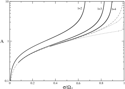
The frequencies derived for modes outside corotation confirm the results of Rezzolla & Yoshida (2001). As the amount of differential rotation increases, the frequencies of the r-modes decrease and approach corotation. The code crashes as at the equator, crashing at larger values of for modes that at uniform rotation have larger . Modes that have very large in uniform rotation are not shown, but follow the general trend illustrated in the figures. Whether modes continue to exist very close to the corotation boundary as the degree of differential rotation is increased still further is difficult to say. We have however tracked modes very close to the corotation boundary and our results suggest that modes outside corotation cease to exist below a certain value of . Disappearance of modes as a system parameter changes is not unexpected. Several examples of eigenvalues vanishing when parameters change are given in Kato (1995).
The question of whether modes can enter the corotation region by developing equatorial corotation points was discussed in section 7.2. For this law the maximum value of is 1. This means that, analytically, we were able to rule out any even solutions with equatorial corotation points for any value of , and any odd solutions for . This was confirmed by our numerical results. For we were not able to rule out analytically the possibility of odd r-modes crossing the boundary. Our numerical results suggest however that there are no odd r-mode solutions existing below . For this rotation law, therefore, we find no evidence that r-modes cross into corotation.
8.3 Case 2: The v-constant rotation law
Another law that has been examined in the literature is the v-constant rotation law. There are however two different laws with this name in the literature. The first, used by Hachisu (1986) and Karino & Eriguchi (2002), takes the form
| (58) |
The second, used by Eriguchi & Müller (1985), Karino, Yoshida & Eriguchi (2001), and Rezzolla & Yoshida (2001), takes the form
| (59) |
In both cases uniform rotation () is reached in the limit . For the first law it is not possible to have , so we can rule out the possibility of dynamically unstable modes or stable modes within corotation. For the second, can be zero for or , so we cannot a priori rule out the possibility of unstable modes. No instabilities were found, however, by our numerical analysis. In fact the modes and continuous spectrum for the two v-constant laws behave qualitatively identically to the modes and continuous spectrum of the j-constant law. For this reason we have not included figures of the results.
8.4 Case 3: Wolff’s solar rotation law
Wolff’s solar rotation law (Wolff, 1998) takes the form
| (60) |
The parameter measures the amount of differential rotation, uniform rotation corresponding to . Wolff considers the range but we will consider an upper limit of as there are interesting phenomena in this range. The rotation rate for this law is lowest at the pole. We get
| (61) |
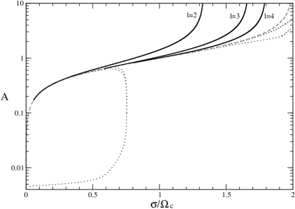
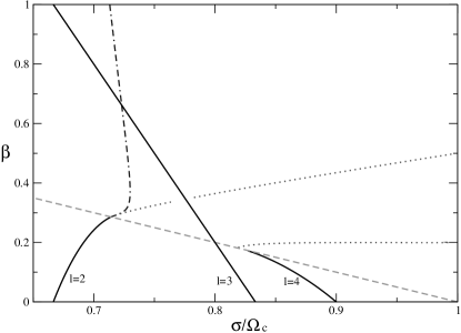
In this case has a zero on the domain for . Both dynamical instabilities and regular solutions in corotation are therefore possible.
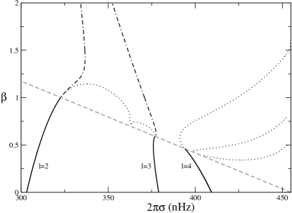
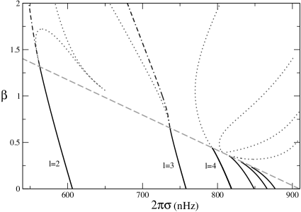
Figure 2 shows the frequencies of a selection of modes and zero-step corotating solutions for and . As the amount of differential rotation increases, the frequency of the each r-mode shifts and in due course all modes encounter the corotation boundary. Modes of low appear to approach the boundary directly, modes of higher seem to approach tangentially. Searching for mode solutions on the corotation boundary, as described in section 7.1, we find valid solutions at the points where the and modes encounter the boundary, suggesting that these modes can develop corotation points222Figure 2 appears to suggest that the mode crosses the boundary. There is however no physically valid solution on the boundary. Resolving this region in more detail it is possible to see the mode and the corresponding zero-step corotating solution approaching the boundary tangentially but not crossing.. As increases so does the number of valid solutions on the corotation boundary. For and there are valid solutions at the point where the four lowest modes encounter the corotation boundary. Modes of larger , which appear to approach tangentially, do not seem to cross the boundary.
A numerical search for modes that are regular in corotation but for which the corotation point does not coincide with the zero of proved fruitless. For the range of examined there were no valid solutions on the domain (see the discussion in Section 8.1).
What about the possibility of regular solutions, with corotation points at the point where ? Such solutions could only exist at one frequency for a given , this frequency being a smooth function of . If we represent the solution as a sum over spherical harmonics, , it is possible to derive a recursion relation for the coefficients . A numerical search for these modes yields nothing, however, and a numerical examination of the coefficients shows why. The coefficients are divergent, with as . There are therefore no regular modes in corotation for this law.
Continuous spectrum solutions with zero-step in the first derivative are present for this rotation law. Such solutions are generated at the point where real-frequency modes appear to enter corotation (i.e. where there are valid solutions on the corotation boundary). There are also many such solutions present at low differential rotation which, in contrast, seem to approach both edges of the corotation region tangentially.
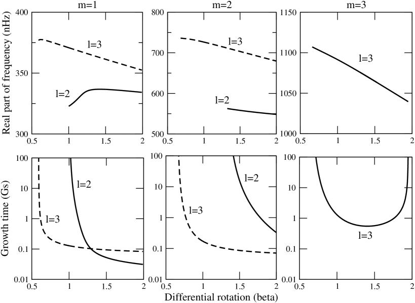
Dynamical instabilities are found to develop at the point where modes encounter the corotation boundary at values of for which has a zero on the shell (in accordance with the instability criterion derived in Section 5). Modes that encounter the corotation boundary below the threshold value of do not exhibit instabilities. There are five unstable modes, corresponding to and . We find no instabilities for modes of higher or . Frequencies and growth times for these unstable modes are shown in figure 3. The behaviour of the mode is particularly interesting as it indicates that the mode becomes stable again for high differential rotation. The mode exhibits similar behaviour at higher .
We can see from equations (25) and (61) why we should not expect to find any unstable modes at high . As increases, the negative part of will come to dominate the integrand in equation (25). Beyond a certain threshold value it will no longer be possible to satisfy the integral equation. The precise value of the threshold will depend on but all modes will reach this point for some .
The results reported in this paper agree with those reported by Wolff for real-frequency modes outside corotation. However, they differ dramatically for solutions with corotation points. In addition, we find dynamical instabilities not mentioned by Wolff. The discrepancy between the results likely originates with Wolff’s perturbation method and with his choice of basis eigenfunctions. He uses not only the standard r-mode eigenfunctions discussed in section 3 but a set of toroidal geostrophic eigenfunctions of single . But the geostrophic solutions form a degenerate set in uniform rotation and cannot be classed as eigenfunctions. As such they cannot be used as a basis for perturbation.
We can compare the results from our investigation with measurements of the degree of differential rotation at various depths in the Sun (Howe et al, 2000). The degree of differential rotation is highest in the surface layers and the convective envelope, where values of nHz and nHz are reported. This would correspond to having . At this level in our model we see dynamically unstable modes, the fastest having a growth time of just a few years.
Our model is very simplistic. It does not, for example, include viscosity, which would be expected to shift the points of marginal stability to a higher degree of differential rotation. However, in the outer layers of the Sun the degree of differential rotation is almost independent of the radius, suggesting that a shell model may not be a bad approximation. In this case a dynamical instability of the type found in this model could be involved in limiting the degree of differential rotation observed in the Sun. See also Dzhalilov, Staude & Oraevsky (2002) for a discussion of various Solar properties that might be explained by the action of unstable r-modes with growth times of years. Whether dynamical instabilities of the type found in this paper could play a similar role is an open question.
8.5 Case 4: A simple quadratic rotation law
The fourth rotation law we have considered takes the form
| (62) |
Here the parameter measures the degree of differential rotation and we have examined the range . Uniform rotation () is recovered if . As with Wolff’s law the rotation rate for this law is greatest at the equator. We get
| (63) |
From this we see that has a zero on the domain if . Both dynamical instabilities and regular solutions in corotation are therefore possible. Figure 4 shows the frequencies of a selection of modes and zero-step corotating solutions for and .
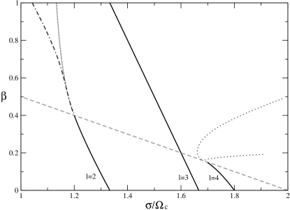
Just as for Wolff’s law, modes of low approach the corotation boundary directly as differential rotation is increased. Modes of higher tend to approach tangentially. And in accordance with this there are valid solutions on the corotation boundary for the and modes.
The mode is a little different however, as it passes straight into corotation as a regular mode. To see why this happens consider the following argument. For this rotation law we can write
| (64) |
and
| (65) |
As discussed in section 6.1, the zeroes of these two functions may coincide, making the governing equation regular and giving rise to regular solutions in corotation. This will occur if
| (66) |
In this case the governing equation (23) becomes
| (67) |
This equation is simply Legendre’s equation for . Thus there is a pure mode that corotates but is completely regular. Just as for Wolff’s law, however, there are no regular corotating solutions of the type given in equation (28).
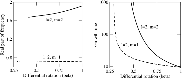
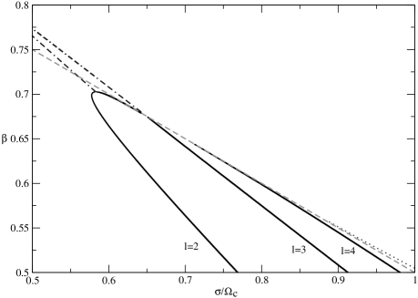
Only the and modes become dynamically unstable at the point where they encounter the corotation boundary. These are the only modes that hit the boundary after passing the threshold value of for which first has a zero on the shell. Frequencies and growth times for both modes are shown in figure 5.
8.6 Case 5: A simple trigonometric rotation law
The final rotation law we have considered is
| (68) |
The parameter measures the degree of differential rotation and we have examined the range . Uniform rotation () is recovered if . The rotation rate for this law is greatest at the pole, as it is for the j-constant and v-constant laws. What is different about this law, however, is that for , which could permit dynamical instabilities. Figure 6 shows mode frequencies for for a reduced range of the differential rotation parameter . The figure shows interesting phenomena that we do not see for any of the other rotation laws. Modes crossing the corotation boundary for this law would have to develop equatorial corotation points, as discussed in section 7.2. For this law, the maximum value of is 2. Modes of odd symmetry can in principle cross the boundary if , modes of even symmetry if .
Let us start by considering the mode. As the amount of differential rotation is increased, the frequency approaches the corotation boundary. The mode crosses the corotation boundary above the instability threshold value of , and above this point continues to exist as a dynamically unstable mode. An odd zero-step solution also develops at this point, but this is not shown in Figure 6, as the frequency is very close to the real part of the frequency of the dynamically unstable mode.
The situation for the even modes is slightly different. Although the modes could in principle cross the corotation boundary, we find that the and modes merge outside corotation, becoming dynamically unstable. Such a route to instability is not seen for the other rotation laws examined. With reference to Figure 6, note that we were unable to track the mode for because the frequency was too close to the corotation boundary. We are however confident that it is this mode that is merging with the mode, for three reasons. Firstly, the merging mode has even symmetry (as we would expect). Secondly, all even modes with approach the corotation boundary at lower values of . The mode is the only other even mode apart from that appears to persist to high . Thirdly, the merging mode is not emerging from corotation, as the only valid solution on the corotation boundary for occurs at the point where the mode crosses. The most reasonable conclusion is that the mode continues to exist just outside corotation for before moving away from the boundary to merge with the mode at higher .
9 Summary
The oscillations of neutron stars are thought to be a promising source of gravitational waves. In order to develop accurate models of gravitational wave emission we need to develop a full understanding of the dynamics of these stars. One factor that has been neglected in many previous studies is differential rotation. Neutron stars are thought to be born with differential rotation, and there are several plausible mechanisms that could sustain differential rotation beyond birth. Differential rotation introduces the possibility of dynamical shear instabilities (Papaloizou & Pringle, 1984, 1985). In addition, the perturbation equations of differentially rotating inviscid systems are complicated by the presence of singularities at points where the pattern speed of a mode equals the local angular velocity of the background flow. These singularities mean that differentially rotating inviscid systems possess a continuous spectrum in addition to discrete modes. To begin to understand this problem we have in this paper analysed the normal mode problem for a toy model, a differentially rotating shell. Although the model is simplistic, it exhibits many of the key features of the more complex three-dimensional problem.
In the uniform rotation limit the shell problem admits the standard r-modes as solutions. As the degree of differential rotation increases the frequencies of these modes gradually approach the lower edge of the expanding corotation band (). Modes that cross the corotation boundary are found to be rare. Indeed, we can rule out completely the crossing of even modes for certain rotation laws. For other rotation laws and symmetries we find crossings only for modes that have low in the uniform rotation limit. All other modes approach the boundary tangentially and appear to cease to exist when the degree of differential rotation exceeds a threshold value. Modes that have higher in the uniform rotation limit cease to exist at lower degrees of differential rotation.
For frequencies in the corotation band the shell problem admits a continuous spectrum of corotating solutions with discontinuous first derivatives. Although such solutions may appear at first sight unphysical, they will have physical significance when we consider the initial value problem. In general, corotating solutions have both a logarithmic singularity and a finite step in the first derivative at the corotation point. For certain special frequencies, however, the step in the first derivative vanishes. In differentially rotating cylinders these zero-step solutions can merge to give rise to dynamical instabilities (Balbinski, 1985), but we observe no such behaviour in our problem for the rotation laws examined. We cannot rule out the possibility, however, for other rotation laws.
The character of the modes that cross into corotation varies. At all points where modes cross the corotation boundary we observe the development of zero-step corotating solutions (except in one unique case, discussed below). At some points we also observe the development of dynamically unstable modes. A necessary (but not sufficient) condition for dynamical instability is that be zero somewhere on the shell. For the rotation laws examined this condition is met only when the degree of differential rotation exceeds a threshold value. All modes crossing the corotation boundary above this threshold become dynamically unstable. We also observe, for one rotation law, the development of a dynamical instability via the merger of two stable modes outside corotation. Only in one exceptional case for the simplest rotation law did we observe a mode crossing the corotation boundary and continuing to exist as a regular stable mode. Such regular corotating modes are unlikely to exist for more realistic rotation laws.
Before moving on to the three-dimensional problem, we intend to investigate two related problems for the simple shell model. The first factor of interest is the effect of viscosity, an essential component of any realistic model. If we consider the Navier-Stokes equations instead of the Euler equations the vorticity equation for the stream function becomes
| (69) |
where is the coefficient of shear viscosity. Equation (9) is not singular, as the coefficient of the leading derivative is never zero. So in the viscous problem there is no continuous spectrum, simply sets of discrete modes. In the zero viscosity limit, however, the solutions to the viscous problem should reduce to the modes and continuous spectrum of the inviscid problem. At first sight it is difficult to see how discrete well-behaved modes could reduce to the singular continuous spectrum solutions that we derived for the inviscid problem in Section 6.2. Boyd (1981) resolves this difficulty by noting that any physical continuous spectrum perturbation is made up of an integral over frequency of the singular inviscid solutions. When solving the viscous problem, the modes are discrete for even the tiniest viscosity and no integration over frequency is required. Solution of the viscous problem should therefore shed light on the physical manifestation of the continuous spectrum.
We are also pursuing the initial value problem. It is clear from our analysis of the normal mode problem that the time dependence of the continuous spectrum will only be understood by solving the initial value problem. In fact the singular continuous spectrum solutions found in this paper only acquire physical meaning when we consider the evolution of initial data. We are particularly interested to see whether the zero-step solutions appear physically distinct in time evolutions. That the zero-step solutions might exhibit different time-dependence is suggested by the fact that these solutions have zero Wronskian, which will contribute an additional pole to the integrand of the Laplace Transform inversion integral (Watts et al, in preparation). We also hope that an analysis of the initial value problem will enable us to develop necessary and sufficient conditions for instability.
10 Acknowledgements
We would like to thank Luciano Rezzolla, Shin’ichirou Yoshida and Emanuele Berti for helpful comments. We also acknowledge support from the EU Programme ’Improving the Human Research Potential and the Socio-Economic Knowledge Base’ (Research Training Network Contract HPRN-CT-2000-00137). AW is supported by a PPARC postgraduate studentship and NA acknowledges support from the Leverhulme Trust in the form of a prize fellowship and PPARC grant PPA/G/1998/00606.
References
- Abramowicz, Rezzolla & Yoshida (2002) Abramowicz M.A., Rezzolla L., Yoshida S., 2002, Class.Quant.Grav., 19, 191
- Balbinski (1984a) Balbinski E., 1984, MNRAS, 209, 145
- Balbinski (1984b) Balbinski E., 1984, MNRAS, 209, 721
- Balbinski (1985) Balbinski E., 1985, MNRAS, 216, 897
- Balmforth & Morrison (1999) Balmforth N.J., Morrison P.J., Studies in Applied Math., 102, 309
- Baumgarte, Shapiro & Shibata (2000) Baumgarte T.W., Shapiro S.L., Shibata M., 2000, ApJ, 528, L29
- Boyd (1981) Boyd J.P., 1981, J.Math.Phys., 22, 1575
- Centrella et al (2001) Centrella J.M., New K.C.B., Lowe L.L., Brown D.J., 2001, ApJ, 550, L193
- Dzhalilov, Staude & Oraevsky (2002) Dzhalilov N.S., Staude J., Oraevsky V.N., 2002, A&A, 384, 282
- Dimmelmeier, Font & Müller (2002) Dimmelmeier H., Font J.A., Müller E., 2002, A&A, 388, 917
- Drazin & Reid (1982) Drazin P.G. Reid, W.H., 1982, Hydrodynamic stability, Cambridge Univ. Press, Cambridge
- Eriguchi & Müller (1985) Eriguchi Y., Müller E., 1985, A&A, 146, 260
- Friedman & Schutz (1978a) Friedman J.L., Schutz B.F., 1978, ApJ, 221, 937
- Friedman & Schutz (1978b) Friedman J.L., Schutz B.F., 1978, ApJ, 222, 281
- Fujimoto (1993) Fujimoto M.Y., 1993, ApJ, 419, 768
- Hachisu (1986) Hachisu I., 1986, ApJSS, 61, 479
- Haurwitz (1940) Haurwitz B., 1940, J. Mar. Res., 3, 254
- Howe et al (2000) Howe R., Christensen-Dalsgaard J., Hill F., Komm R.W., Larsen R.M., Schou J., Thompson M.J., Toomre J., 2000, Sci, 287, 2456
- Imamura et al (1995) Imamura J.N., Toman J., Durisen R.H., Pickett B.K., Yang S., 1995, ApJ, 444, 363
- Karino & Eriguchi (2002) Karino S., Eriguchi Y., 2002, ApJ, 578, 413
- Karino, Yoshida & Eriguchi (2001) Karino S., Yoshida S., Eriguchi Y., 2001, Phys. Rev. D., 64, 024003
- Kato (1995) Kato T., 1995, Perturbation theory for linear operators, Springer-Verlag, Berlin
- Levin & Ushomirsky (2001) Levin Y., Ushomirsky G., 2001, MNRAS, 322, 515
- Lindblom, Tohline & Vallisneri (2001) Lindblom L., Tohline J.E., Vallisneri M., 2001, Phys. Rev. Lett., 86, 1152
- Luyten (1990a) Luyten P.J., 1990, MNRAS, 242, 447
- Luyten (1990b) Luyten P.J., 1990, MNRAS, 245, 614
- Luyten (1991) Luyten P.J., 1991, MNRAS, 248, 256
- New & Shapiro (2001) New K.C.B., Shapiro S.L., 2001, ApJ, 548, 439
- Papaloizou & Pringle (1984) Papaloizou J.C.B., Pringle J.E., 1984, MNRAS, 208, 721
- Papaloizou & Pringle (1985) Papaloizou J.C.B., Pringle J.E., 1985, MNRAS, 213, 799
- Rezzolla et al (2000) Rezzolla L., Lamb F.L., Shapiro S.L., 2000, ApJ, 531, L139
- Rezzolla & Yoshida (2001) Rezzolla L., Yoshida S., 2001, Class. Quant. Grav., 18, L87
- Shapiro & Teukolsky (1983) Shapiro S.L., Teukolsky S.A., 1983, Black Holes White Dwarfs and Neutron Stars, Wiley
- Schutz (1980) Schutz B.F., 1980, MNRAS, 190, 7
- Shibata & Uryu (2000) Shibata M., Uryu K., 2000, Phys. Rev. D, 61, 064001
- Shibata, Baumgarte & Shapiro (2000) Shibata M., Baumgarte T.W., Shapiro S.L., 2000, ApJ, 542, 453
- Shibata, Karino & Eriguchi (2002) Shibata M., Karino S., Eriguchi Y., 2002, MNRAS, 334, L27
- Stewartson & Rickard (1969) Stewartson K., Rickard J.A., 1969, J. Fluid Mech., 1969, 35, 759
- Tassoul (1978) Tassoul J.L., 1978, Theory of rotating stars, Princeton Univ. Press, Princeton, NJ
- Van Kampen (1955) Van Kampen N.G., 1955, Physica, 21, 949
- Watts & Andersson (2002) Watts A.L., Andersson N., 2002, MNRAS, 333, 943
- Wolff (1998) Wolff C.L., 1998, ApJ, 502, 961
- Yoshida et al (2002) Yoshida S., Rezzolla L., Karino S., Eriguchi Y., 2002, ApJ, 568, L41
- Zwerger & Müller (1997) Zwerger T., Müller E., 1997, A&A, 320, 209