Weak Lensing Discovery and Tomography of a Cluster at $z=0.68$

Abstract

We report the weak lensing discovery, spectroscopic confirmation, and weak lensing tomography of a massive cluster of galaxies at $z=0.68$, demonstrating that shear selection of clusters works at redshifts high enough to be cosmologically interesting. The mass estimate from weak lensing, $11.1\pm 2.8\times 10^{14}\ (r/Mpc)\ M_{\odot}$ within projected radius $r$, agrees with that derived from the spectroscopy ($\sigma_{v}=980$ km s^-1), and with the position of an arc which is likely to be a strongly lensed background galaxy. The redshift estimate from weak lensing tomography is consistent with the spectroscopy, demonstrating the feasibility of baryon-unbiased mass surveys. This tomographic technique will be able to roughly identify the redshifts of any dark clusters which may appear in shear-selected samples, up to $z\sim 1$.

1 Introduction

Galaxy clusters are important tools for studying the formation of structure over cosmic time and for probing cosmological parameters (Haiman, Mohr & Holder 2001). Such studies depend crucially on the selection of unbiased samples of clusters covering a broad mass and redshift range. (“Cluster” here indicates any mass concentration, regardless of galaxy or gas content, as mass is the most important parameter for cosmological tests.) The most well-established selection techniques are based on emission of visible-wavelength light from member galaxies (Gladders & Yee 2000 and references therein) or of X-rays from hot intracluster gas (Borgani & Guzzo 2001 and references therein). A newer technique uses the Sunyaev-Zel’dovich effect, in which the cosmic microwave background is modified in its passage through the intracluster medium (Carlstrom, Holder & Reese 2002 and references therein). Each of these methods depends on the presence of baryons and on other physical conditions within the cluster and therefore may introduce some bias.

In contrast, weak lensing (see Bartelmann & Schneider 2001 for a review) has the potential to select clusters independent of their baryon content, dynamical state, and star formation history (Schneider 1996). However, surveying for clusters via shear selection is still in its infancy. The only shear-selected mass with a spectroscopic redshift is at $z=0.27$ (Wittman et al. 2001, hereafter W2001), whereas cosmological effects on cluster abundances are expected to become significant only well above this redshift. More recently, Dahle et al. (2003) and Schirmer et al. (2003) each identified several shear-selected masses with redshifts determined from two-color photometry as $z\sim 0.5$. In other cases, (Erben et al. 2000; Umetsu & Futamase 2000; Clowe, Trentham & Tonry 2001; Miralles et al. 2002), the object causing the shear has not been assigned a redshift. Weinberg & Kamionkowski (2003) calculate that up to 20% of clusters in shear-selected surveys are expected to be optically dark. However, without a redshift, the masses of these “dark clusters” cannot be computed. Hence mass-to-light ratios (or even limits) cannot be computed either, and it is unclear just how dark these clusters are. Nonspectroscopic means of determining their redshifts (and therefore masses and derived parameters) must be developed.

Here we report the discovery of a shear-selected cluster at $z=0.68$, which demonstrates that this technique can cover a significant redshift range. As in W2001, we also derive a lens redshift from weak lensing tomography, by fitting the relation between shear and source photometric redshift. This redshift agrees with the spectroscopic value, but is derived entirely independently. This is the first demonstration that even high-redshift “dark” clusters could be assigned redshifts, thus making them cosmologically useful. The observations were obtained as part of the Deep Lens Survey (DLS) and cover only a few percent of its area. When complete, the survey will yield a sample of $\sim 200$ shear-selected clusters.

2 Imaging and Photometric Redshifts from the Deep Lens Survey

The DLS (Wittman et al. 2002; see also http://dls.bell-labs.com) is an ongoing deep $BVR{z^{\prime}}$ imaging survey of six 2${}^{\circ}\times 2^{\circ}$ fields using the Mosaic imagers on the KPNO and CTIO 4-m telescopes. With total exposure times in $BVR{z^{\prime}}$ of 12, 12, 18, and 12 ksec respectively, it will reach a depth of 29, 29, 29, and 28 mag arcsec^-2. The $R$ filter is used when the seeing is 0.9${}^{\prime\prime}\,$ or better, to optimize its utility for lensing studies. All shape measurements are done in $R$, where the enforced good seeing will provide a shear-selected survey which is more uniform and more sensitive than would be possible with typical atmospheric conditions. The other filters provide color information for photometric redshift estimates, and are observed in when the seeing is worse than 0.9${}^{\prime\prime}\,$. Photometric calibration is provided by observations of standard star fields, using the calibrated catalog of Landolt (1992) for $BVR$ and the most recent calibrated ${z^{\prime}}$ catalog from D. Tucker (private communication).

The Mosaic cameras provide 8k $\times$ 8k pixels subtending 0.257${}^{\prime\prime}\,$ each, for a 35${}^{\prime}\,$ square field. Each 35${}^{\prime}\,$ “subfield” of the survey is imaged with 20 dithered exposures in each filter, with dithers up to 200${}^{\prime\prime}\,$ to provide good flatfielding. Adjacent subfields will be stitched together into full 2^∘ fields after all the contiguous data have been acquired, but for now coaddition and analysis takes place on a subfield-by-subfield basis. For this paper we are considering one particular subfield which has been completed, centered at 10:54:43 -05:00:00 (J2000). Several other subfields have been completed, and shear-selected clusters tentatively identified, but this cluster is the first to receive spectroscopic confirmation. This is due to the presence of the likely strongly lensed arc, which gave us the confidence to arrange for spectroscopy even before the weak lensing analysis was completed. Therefore, this cluster may not be typical of the final DLS shear-selected sample. However, the characteristics of the data, such as number of sources per square arcminute and photometric redshift accuracy, are typical.

We observed this field with the CTIO 4-m Blanco telescope in 2000, 2001, and 2002 as part of the DLS imaging campaign. Full details of the data processing are given in Wittman et al. (2002), but we summarize here. We processed the data through flatfielding with standard tasks from the IRAF package mscred, then registered and combined them with custom software.

Before combining the $R$ images (the only bandpass intended for lensing analysis), we first correct each exposure for point-spread function (PSF) anisotropy using the procedure of Fischer & Tyson (1997). This is necessary for each exposure because some observing conditions, such as focus and guiding errors, change from exposure to exposure. Even within an exposure, the procedure is applied separately for each CCD, in case there are piston differences between the CCDs. Briefly, the procedure is to find stars based on their locus in the magnitude-size diagram; derive a fit to the spatial variation of the PSF moments, clipping outliers which tend to be interloping galaxies; and convolve the image with a kernel which, at each point, is aligned orthogonal to the interpolated PSF at that point. Each CCD typically has 50–100 unsaturated, unambiguous stars, which provide for a second-order polynomial fit to the spatial variation. We also apply this procedure to the combined $R$ image, to reduce the effects of any small registration errors. In this case, we find $\sim 1000$ stars and use a fourth-order polynomial fit. The full-width at half-maximum (FWHM) of the $R$ image, after all combines and convolutions, is 0.96 arcsec. For comparison, the FWHM of the unconvolved $B$, $V$, and ${z^{\prime}}$ images are 1.03, 0.96, and 1.39 arcsec respectively.

To produce photometric redshifts, we make matched-isophote catalogs with detection in $R$ band using SExtractor (Bertin & Arnouts 1996), and use the photometry as input to a modified version of the HyperZ photometric redshift package (Bolzonella, Miralles & Pelló 2000). The modification is an important one for the DLS. Because of the limited filter set, there are some color degeneracies. That is, the observed colors of a galaxy may be as well matched to one template at low-redshift as to another template at high redshift. Therefore we add a luminosity function prior, as described in W2001, which generally resolves the ambiguity (see Benitez 2000 for detailed examples). The DLS filter set differs from that of W2001, so we used different luminosity function parameters, $M_{R}^{*}=-22.0$ and $\alpha=-1.24$. We adopt a cosmology in which $H_{0}=70$, $\Omega_{m}=0.3$, and $\Omega_{\Lambda}=0.7$ throughout this work.

We verified the accuracy of the photometric redshifts in this subfield by comparison with spectroscopic redshifts of 22 galaxies in the range $0.36<z_{\rm spec}<0.98$ obtained at Keck (see Section 4), plus 49 galaxies in the range $0.04<z_{\rm spec}<0.36$ from the 2dFGRS public data (Colless et al.  2001). Thus the full spectroscopic sample for this 35${}^{\prime}\,$ subfield contains 71 galaxies in the range $0.04<z_{\rm spec}<0.98$. Like many other authors, we measure the difference between photometric and spectroscopic redshifts in terms of the quantity $\delta z=(z_{\rm spec}-z_{\rm phot})/(1+z_{\rm spec})$, which is just the percentage error in the quantity $1+z_{\rm spec}$. This encodes the fact that a redshift error of a given size is more important at low redshift than at high redshift.

Figure 1 shows a scatterplot of $\delta z$ versus $z_{\rm spec}$. The rms value of $\delta z$ is 0.065, and the range is $-0.16<\delta z<0.16$. This per-galaxy accuracy is sufficient for lensing work, because it is significantly less than the inherent shape noise in each galaxy. This is reflected in the design of the DLS, which emphasizes area coverage and depth rather than an extended filter set. Similar results are obtained with a much larger spectroscopic sample in a separate DLS field (Margoniner et al., in preparation).

In this subfield, the mean value of $\delta z$ averaged over all redshifts is consistent with zero ($-0.0014\pm 0.0077$), indicating negligible bias. However, the mean value obscures a tendency to overpredict very low redshifts and underpredict redshifts near that of the cluster. For example, the mean $z_{\rm phot}$ of cluster members is 0.60, as compared to the spectroscopic value of 0.68 which will be derived in Section 4. We do not attempt to correct for this trend here, as part of our purpose is to demonstrate how well weak lensing tomography will work over very large areas without spectroscopic feedback. Due to the breadth of the lensing kernel, an error of this size is still less than the statistical error in locating a lens along the line of sight.

Photometric redshifts derived from this filter set are expected to degrade for $z>1.6$, because the 4000 Å break is shifted through the ${z^{\prime}}$ filter. We have no spectroscopic data to confirm such high redshifts in this field, so we limit our analysis to sources with $z_{\rm phot}<1.6$.

3 Weak lensing detection

We measured weighted moments of objects in $R$ using the ellipto software described in Bernstein & Jarvis (2002), discarding any sources which triggered error flags. We also used their seeing correction procedure, discarding sources which were not at least 25% larger than the PSF. We further winnowed the sources by requiring a maximum observed ellipticity of 0.5 (rejecting about $15\%$ of sources), because with $\sim$ 1${}^{\prime\prime}\,$ resolution, highly elliptical objects are quite likely to be blends of two distinct sources, based on measurements of the Hubble Deep Field and synthetic fields convolved with this seeing. The number of sources passing all these quality checks is 45435, or 37 arcmin^-2.

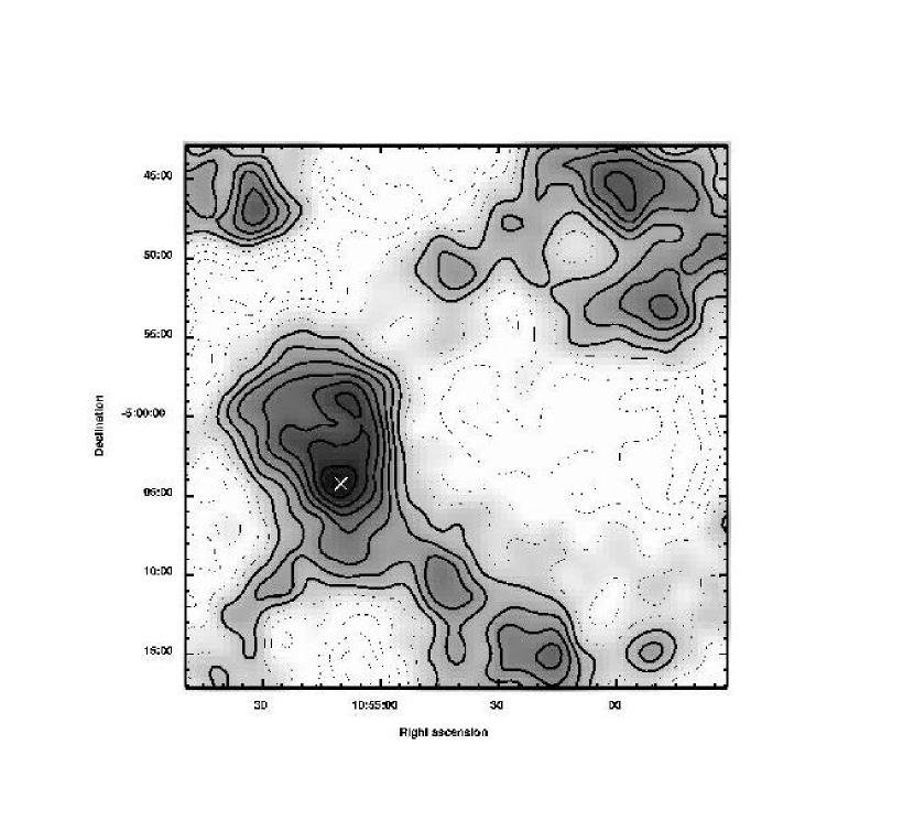
Figure 2: Projected mass map of the 35${}^{\prime}\,$ field, smoothed with a 30${}^{\prime\prime}\,$ rms Gaussian. Black indicates the most dense regions (the units are arbitrary). Contours are equally spaced from the lowest to the highest value; negative and zero contours are drawn more thinly than positive contours. Note that only departures from the mean density are measured, so that negative contours represent underdensities. The main mass concentration is coincident with a cluster in which the brightest galaxy (location marked with an X) is only 23${}^{\prime\prime}\,$ from the peak projected mass density.

We discovered the cluster before we had photometric redshift information, by making a convergence map from $R$-selected sources, using the method of Fischer & Tyson (1997). Figure 2 shows a convergence map made from selecting the 17163 sources with $23<R<25$ from the final catalog, with 30${}^{\prime\prime}\,$ pixels and smoothed with a 30${}^{\prime\prime}\,$ rms Gaussian. A dominant mass concentration appears in the figure, peaking at 10:55:11.6, -05:04:16 (all coordinates in this paper are J2000). Maps made from redshift-selected catalogs appear similar to this one. We show the $R$-selected map to demonstrate that the weak lensing detection of this cluster does not depend on photometric redshifts in any way. We defer a discussion of the significance of the detection to Section 5, where we will take full advantage of the redshift information.

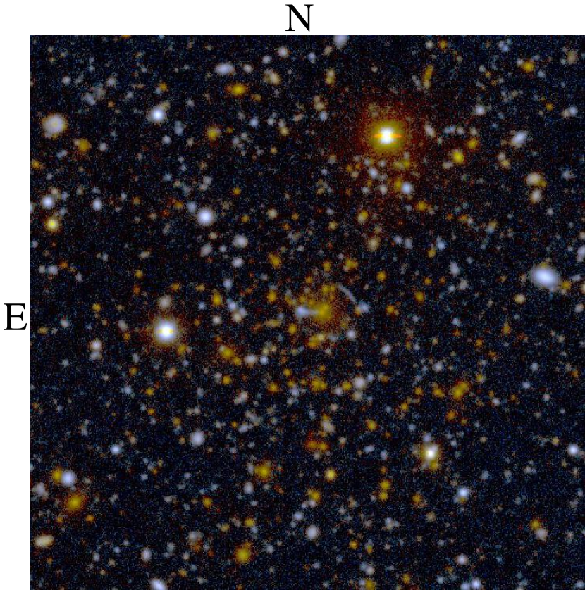
Figure 3: A 3${}^{\prime}\,$ square section of the $R$ image (of a BVR color composite in the electronic edition), centered on the BCG. The BCG is $R=20.6$, and the faintest galaxies visible in this reproduction are $R\sim 26$. North is up, and east to the left. The possible strong lensing arc is 10${}^{\prime\prime}\,$ to the northwest of the brightest cluster galaxy.

The multicolor imaging shows a concentration of red galaxies near the location of the mass peak, with the brightest cluster galaxy (BCG) at 10:55:10.1 -05:04:13. Figure 3 shows a 3${}^{\prime}\,$ square section of the $R$ image (of a $BVR$ color composite in the electronic edition), centered on the BCG. The BCG is 23${}^{\prime\prime}\,$ from the mass peak, well within the 1$\sigma$ mass peak positional uncertainty of 58${}^{\prime\prime}\,$ derived from bootstrap resampling and from mass maps made from a variety of similar, but statistically independent subcatalogs representing different photometric redshift ranges. Therefore we tentatively identify the cluster with the mass concentration. Neither the cluster nor any apparent members are listed in the NASA/IPAC Extragalactic Database or in the ROSAT All-Sky Survey Source Catalog.

Ten arcseconds to the northwest of the brightest cluster galaxy appears an arc, which based on morphology alone is likely to be a strongly lensed background galaxy. Its redshift is unknown, but it is bluer than the cluster members, consistent with the lensing hypothesis.

4 Spectroscopic Confirmation

We took spectra of 24 likely member galaxies (with a projected position near the cluster and in the magnitude range $20.7<R<22.6$) with the Low-Resolution Imaging Spectrograph (LRIS, Oke et al.  1995) at W. M. Keck Observatory in November, 2000. Positions, $R$ magnitudes, redshifts, and spectral type and quality (following the system of Cohen et al.  1999) are listed in Table 1. Seventeen had redshifts in the range 0.664–0.694, representing a cluster with a mean redshift of 0.68. The remaining seven are foreground and background galaxies in the redshift range 0.36–0.98. Among the cluster members, the line-of-sight velocity dispersion is $980\pm 240$ km s^-1 using the biweight estimator of Beers et al.  (1990). The effect of membership uncertainty is modest: elimination of the most deviant galaxy results in a biweight estimate of 840 km s^-1. We stress that the spectroscopy is used only as confirmation, not as input to the photometric redshift and lensing procedures.

The density of points in Figure 1 seems to reveal a second cluster, at $z=0.08$. However, the galaxies at that spectroscopic redshift are spread over the entire field and do not appear to form a coherent cluster or group. Furthermore, we find no evidence for such a cluster in the lensing analysis below. In any case, the sensitivity of the lensing analysis to such a low-redshift cluster would be low. Whether this feature is an artifact of the 2dFGRS target selection procedure, an extremely diffuse group, or the outskirts of a cluster outside the field, we conclude that it does not affect the lensing analysis.

5 Weak Lensing Tomography

As in W2001, we summarize the tangential shear $\gamma_{t}$ due to the lensing cluster with a single number for each source redshift bin. We do this by separating the catalog into a series of source redshift slices, then for each slice we compute the tangential shear for a series of annuli centered on the BCG, fit a singular isothermal sphere (SIS) profile to that data, and take the value of this fit (and its uncertainty) at 1 Mpc projected radius.

Figure 4 shows $\gamma_{t}$ as a function of source photometric redshift. The results are consistent with a lens at $z=0.68$ (dashed line); the best-fit lens redshift is 0.55 (dotted line). The full lens redshift probability distribution is shown in Figure 5. The mean and rms of this distribution are 0.64 and 0.29 respectively. We also performed several null tests. In the first, we rotated each source by 45^∘ and repeated the analysis. In the second null test, we repeated the analysis about random centers. In all these cases, the lens redshift probability distribution is flat, with the best-fit lens at any redshift having zero mass. In contrast, under the zero-mass hypothesis the $\chi^{2}$ of the data in Figure 4 is 22.4 for 7 degrees of freedom, implying a probability of 0.2%. This is the best estimate of the statistical significance of the discovery, taking advantage of both redshift and shear information: We have 99.8% confidence that these data would not have arisen without a real lens.

Similar results, within the errors given, are obtained when using NFW (Navarro, Frenk & White 1997) profiles, changing the annular binning scheme (by default, three logarithmically-spaced bins from 50${}^{\prime\prime}\,$ to 30${}^{\prime}\,$), varying the center by $\pm$1 arcminute, or changing the redshift binning scheme provided the sampling is adequate. We use fixed-width redshift bins 0.2 wide, which gives a variable number of sources per bin (from 653 to 4490 sources, increasing with redshift), but maintains good redshift sampling.

Note that we have neglected redshift bins above 1.6 due to the limitations of the filter set. We must also guard against sources at $z>1.6$ contaminating the lower-redshift bins. This cannot be done in all generality, but with a lens at known redshift $z_{\rm lens}$, it can be done for $z<z_{\rm lens}$. There, a high rate of contamination by high-redshift sources would increase the shear above its natural value of zero. From the low shear values observed for $z<0.6$ in Figure 4, it would seem that such contamination is not a major factor in the current dataset. Given the large error bars, it is difficult to put a precise limit on the contamination in the current dataset (though we note that the very large error bars in the lowest redshift bin reflect the paucity of sources, itself an indication that high-redshift contamination is limited). For the DLS data as a whole, we will be able to derive limits using a sample of clusters at a variety of redshifts.

6 Mass estimates

A first, rough mass estimate comes from strong lensing. The arc appears at a projected distance of 71 kpc. If this is the Einstein radius, the mass enclosed is $(1.8\times 10^{13}\ M_{\odot}){D_{s}\over D_{ls}}$, where $D_{s}$ and $D_{ls}$ (in Gpc) are the angular diameter distances from observer to source and from lens to source, respectively. ${D_{s}\over D_{ls}}$ could vary from unity (for infinite source redshift) to perhaps five (for a source redshift of 0.9, which is a practical lower limit because the source is unlikely to be in the small volume just behind the cluster).

To compare weak lensing and dynamical measurements on an equal footing, we must adopt a model mass profile. Following W2001 we adopt a singular isothermal sphere (SIS) for its simplicity, as an NFW profile requires an additional parameter but does not significantly improve the fit to the shear profile (see below). The velocity dispersion then implies a projected mass of $7.0\pm 3.4\times 10^{14}\ (r/Mpc)\ M_{\odot}$ within radius $r$, or $5.0\pm 2.4\times 10^{13}\ M_{\odot}$ within 71 kpc, consistent with the strong lensing estimate (all errors quoted are 1$\sigma$).

We estimate the mass using the weak lensing data in two different ways, each time assuming $z_{\rm lens}=0.68$. First, we simply fit the $\gamma_{t}(z_{\rm phot})$ data in Figure 4 for the lens mass, fixing $z_{\rm lens}$ at $0.68$. The result is $11.1\pm 2.8\times 10^{14}\ (r/Mpc)\ M_{\odot}$ within radius $r$, or $7.9\pm 2.0\times 10^{13}\ M_{\odot}$ within 71 kpc, consistent with both strong lensing and dynamical estimates. Equivalently, the velocity dispersion inferred from the lensing data is $1233\pm 155$ km s^-1. Note that using the tomographic lens redshift of 0.55 in the same formalism yields a $\sim 1\sigma$ change in the mass estimate, to $8.7\pm 2.1\times 10^{14}\ (r/Mpc)\ M_{\odot}$.

Alternatively, we attempt to constrain the radial profile more strongly by making a single radial profile using all sources at $0.8<z_{\rm phot}<1.6$, which is more like a traditional weak lensing analysis with a simple foreground/background cut. This radial profile is shown in Figure 6. A straightforward SIS fit to these data (solid line in the figure) yields $8.6\pm 2.3\times 10^{14}\ (r/Mpc)\ M_{\odot}$ within radius $r$, consistent with all the other estimates. The inferred velocity dispersion is $1085\pm 128$ km s^-1. An NFW fit is also shown (dashed line). The SIS fit is slightly better in terms of $\chi^{2}$ per degree of freedom (0.58 with 5 degrees of freedom versus 0.65 with 4 degrees of freedom for the NFW). Given that both are acceptable fits, use of the simpler one-parameter SIS model throughout this paper is justified.

Finally, we estimate the mass-to-light (M/L) ratio using the first weak lensing mass quoted above. We measured the light in $z^{\prime}$ band, which roughly corresponds to emitted $V$ band. This time we made catalogs in single-image mode on the $z^{\prime}$ image so as not to miss very red sources. We extracted subcatalogs centered on the cluster and on seven control regions, and computed the total magnitude of sources within those regions meeting two criteria: being resolved (eliminating stars), and with a $z^{\prime}$ magnitude between 19.75 (the magnitude of the BCG) and 23.75, beyond which incompleteness starts to set in. The total measured magnitude of the cluster (within a radius of 500 kpc) minus the mean background is $z^{\prime}=15.86\pm 0.18$ mag (the uncertainty comes from variation among the control regions). After applying a small correction for the faint end of the luminosity function which was missed and converting from observed $z^{\prime}$ band to rest-frame $V$ using the approach of Fischer & Tyson (1997), we find a rest-frame $M/L_{V}=574\pm 146$. This value is quoted at a projected radius of 500 kpc, but it does not vary significantly in the projected radius range 250—1000 kpc.

7 Conclusions

We have extended shear selection of clusters to a higher redshift range, which will be cosmologically useful. For example, since dark energy has its largest effect on comoving volume at redshift $\sim$0.5, measurements of the volume-redshift relation via mass cluster counting must bracket this and extend up to $z\sim 1$ (Tyson et al.  2003). Furthermore, using the observed $\gamma_{t}(z_{\rm phot})$ relations, we have identified the redshift of the lens in addition to that of the cluster, and found that they are consistent. Thus any dark clusters which might be found in the DLS can be assigned rough redshifts and masses, a necessary first step in investigating them, as well as including them in cluster-counting cosmological tests.

The mass of the cluster is fairly high, but by no means exceptional. Some examples of more massive clusters at this or higher redshift are MS1054-03 at $z=0.83$, with a velocity dispersion of $\sigma_{v}=1170$ km s^-1 (Tran et al.  1999) and $\sigma_{v}=1311$ km s^-1 inferred from weak lensing (Hoekstra et al.  2000), and CL1604+4304 at $z=0.90$, with $\sigma_{v}\sim 1200$ km s^-1 (Postman, Lubin & Oke 2001). This suggests that even at high redshift, the DLS is sensitive to clusters over a significant range of the mass function. However, any conclusions as to the nature of the overall DLS sample would be entirely premature. This cluster may not be representative, as the large arc was a significant factor in choosing to investigate this cluster first.

The M/L of this cluster is very high, but examples of darker clusters can be found. For example, Fischer (1999) found $M/L_{R}=640\pm 150$ for MS12247+2007, consistent with the earlier measurement of Fahlman et al.  (1994) on the same cluster. Whether shear-selected clusters tend to be systematically underluminous (or more accurately, whether optically-selected clusters tend to be overluminous) is a fascinating question which awaits the compilation of a statistically significant sample. We note that the M/L of the “dark clump” detected by Erben et al.  could be as low as $\sim 400$, depending on its redshift which is still unknown (Gray et al. 2001). Thus the label “dark” may well be misleading if it implies a new class of objects. There may well be a continuous distribution encompassing all these examples as well as optically-selected clusters.

A difficulty with optical M/L ratios is that they depend greatly on star formation history, which tends to obscure the underlying question of how mass is assembled. These astrophysical processes are more directly related to the X-ray properties of clusters, so an even more fascinating question which awaits the compilation of a statistically significant sample is whether shear-selected clusters tend to be X-ray underluminous. This and other shear-selected clusters from the DLS are currently being followed up with Chandra and XMM X-ray imaging.

A cluster of this mass is not unexpected in the volume probed by these data (Rahman & Shandarin 2001), so the number of clusters in the complete DLS could be estimated by scaling up the area sampled here, yielding $\sim$60. However, that is a lower limit because we chose only the single most dominant mass concentration in this area. Preliminary analysis of full-depth areas suggests that about 200 clusters will be found in the DLS. The tightness of constraints on cosmological parameters afforded by a sample of this size, with and without priors from other measurements such as the cosmic microwave background, are being computed (Hennawi & Spergel, in preparation).

Table 1: Spectroscopic Redshifts

RA (J2000)	DEC	mR	Type	Quality	z
Cluster members
10:55:15.4	-05:05:14	20.57	AI	1	0.680
10:55:09.1	-05:06:22	21.15	A	1	0.680
10:55:11.8	-05:05:31	20.89	A	1	0.678
10:55:12.1	-05:04:35	22.23	A	1	0.688
10:55:11.1	-05:04:37	22.24	A	2	0.694
10:55:12.3	-05:04:09	21.35	AI	1	0.679
10:55:10.7	-05:04:18	21.91	A	2	0.681
10:55:10.1	-05:04:13	20.60	A	1	0.677
10:55:10.4	-05:04:12	21.00	A	2	0.674
10:55:08.8	-05:04:01	22.33	A	2	0.669
10:55:08.4	-05:03:31	21.81	A	1	0.688
10:55:06.8	-05:03:18	21.74	A	1	0.680
10:55:02.6	-05:02:03	21.21	I	1	0.675
10:54:57.8	-05:01:50	21.81	I	1	0.664
10:54:55.0	-05:01:07	20.80	I	1	0.670
Non-members
10:55:07.2	-05:03:23	20.20	A	1	0.364
10:55:04.8	-05:02:31	20.72	I	1	0.384
10:55:19.1	-05:04:49	21.24	I	1	0.523
10:55:12.8	-05:04:54	20.93	EI	1	0.720
10:55:05.6	-05:02:53	21.53	A	1	0.728
10:54:55.8	-05:00:41	21.71	A	1	0.731
10:54:59.7	-05:00:52	21.73	E	4	0.984

Figure 1: The quantity $\delta z=(z_{\rm spec}-z_{\rm phot})/(1+z_{\rm spec})$ versus spectroscopic redshift, for the 71 galaxies with spectra. The rms value of $\delta z$ is 0.065, and the range is $-0.16<\delta z<0.16$. This per-galaxy accuracy is sufficient for lensing work, because it is significantly less than the inherent shape noise in each galaxy. The mean $\delta z$ averaged over all redshifts is vanishingly small (-0.0014).

Figure 4: Tangential shear $\gamma_{t}$, centered on the BCG, as a function of source photometric redshift. The dotted curve shows the best-fit lens fixed at the spectroscopic redshift of 0.68, and the dashed curve shows the best fit when the lens redshift is allowed to vary ($z=0.55$).

Figure 5: Lens redshift probability distribution. The peak is at $z=0.55$, the mean is $z=0.64$, and the rms is 0.29. The spectroscopic redshift of the cluster is marked with a vertical line at $z=0.68$. The agreement of the lens redshift with the spectroscopic value indicates that any dark mass concentrations which might be found in the DLS can be assigned rough redshifts (and therefore masses and derived quantities such as M/L) from the lensing information alone.

Figure 6: Radial shear profile of the cluster, using all sources with $0.8<z_{\rm phot}<1.6$, along with best-fit SIS (solid line) and NFW (dashed line) models. The SIS fit is slightly better in terms of $\chi^{2}$ per degree of freedom (0.58 with 5 degrees of freedom versus 0.65 with 4 degrees of freedom for the NFW). Because the SIS model fits the data better with one fewer parameter, it is used throughout this paper. The SIS model shown contains $8.6\pm 2.3\times 10^{14}\ (r/Mpc)\ M_{\odot}$ within radius $r$.

References

- (1) Bartelmann, M. & Schneider, P. 2001, Phys. Rep. 340, 291
- B (90) Beers, T. C., Flynn, K. & Gebhardt, K. 1990, AJ 100, 32
- Benítez (2000) Benítez, N. 2000, ApJ, 536, 571
- (4) Bernstein, G. M. & Jarvis, M. 2002, AJ 123, 583
- (5) Bertin, E. and Arnouts, S. 1996, A&A Supp. 117, 393
- (6) Bolzonella, M., Miralles, J.-M., & Pelló, R. 2000, A&A 363, 476
- Borgani & Guzzo (2001) Borgani, S. & Guzzo, L. 2001, Nature, 409, 39
- (8) Carlstrom, J.E., Holder, G.P. & Reese, E.D., 2002, ARA&A, 40, 643
- Clowe, Trentham, & Tonry (2001) Clowe, D., Trentham, N., & Tonry, J. 2001, A&A, 369, 16
- (10) Cohen, J. G., Hogg, D. W., Pahre, M. A., Blandford, R., Shopbell, P. L. & Richberg, K. 1999, ApJS 120, 171
- (11) Colless, M. et al. 2001, MNRAS 328, 1039
- Dahle et al. (2003) Dahle, H., Pedersen, K., Lilje, P. B., Maddox, S. J., & Kaiser, N. 2003, ApJ, 591, 662
- (13) Erben, T., van Waerbeke, L., Mellier, Y., Schneider, P., Cuillandre, J.-C., Castander, F.J. & Dantel-Fort, M. 2000, A&A 355, 23
- Fahlman, Kaiser, Squires, & Woods (1994) Fahlman, G., Kaiser, N., Squires, G., & Woods, D. 1994, ApJ, 437, 56
- Fischer (1999) Fischer, P. 1999, AJ, 117, 2024
- (16) Fischer, P. & Tyson, J. A. 1997, AJ 114, 14
- (17) Gladders, M. & Yee, H. 2000, AJ 120, 2148
- Gray et al. (2001) Gray, M. E., Ellis, R. S., Lewis, J. R., McMahon, R. G., & Firth, A. E. 2001, MNRAS, 325, 111
- (19) Haiman, Z., Mohr, J. & Holder, G. 2001, ApJ 553, 545
- (20) Hoekstra, H., Franx, M. & Kuijken, K. 2000, ApJ, 532, 88
- (21) Landolt, A. U., 1992, AJ104, 340
- (22) J.-M. Miralles et al. 2002, A&A, 388, 68
- Navarro, Frenk, & White (1997) Navarro, J. F., Frenk, C. S., & White, S. D. M. 1997, ApJ, 490, 493
- (24) Oke, J. B., Cohen, J. G., Carr, M., Cromer, J., Dingizian, A., Harris, F. H., Labrecque, S., Lucinio, R., Schaal, W., Epps, H., & Miller, J. 1995, PASP 107, 307
- (25) Postman, M., Lubin, L. & Oke, B. 2001, AJ 122, 1125
- Rahman & Shandarin (2001) Rahman, N. & Shandarin, S. F. 2001, ApJ, 550, L121
- (27) Schirmer, M., Erben, T., Schneider, P., Pietrzynski, G., Gieren, W., Micol, A. & Pierfederici, F., 2003, A&A, submitted, astro-ph/0305172
- (28) Schneider, P. 1996, MNRAS 283, 837
- Tran et al. (1999) Tran, K. H., Kelson, D. D., van Dokkum, P., Franx, M., Illingworth, G. D., & Magee, D. 1999, ApJ, 522, 39
- (30) Tyson, J.A., Wittman, D., Hennawi, J. & Spergel, D., Nuclear Physics B, 2003, in press; astro-ph/0209632
- Umetsu & Futamase (2000) Umetsu, K. & Futamase, T. 2000, ApJ 539, L5
- (32) Weinberg, N. & Kamionkowski, M. 2003, MNRAS, 341, 251
- (33) Wittman, D., Tyson, J. A., Kirkman, D., Dell’Antonio, I. & Bernstein, G., 2000, Nature 405, 143.
- (34) Wittman, D., Tyson, J. A., Margoniner, V. E., Cohen, J. G. & Dell’Antonio, I., 2001, ApJ 557, L89 (W2001)
- (35) Wittman, D., et al. 2002, Proc. SPIE, 4836, 73; astro-ph/0210118