Extracting cosmic microwave background polarization from satellite astrophysical maps

Abstract

We present the application of the Fast Independent Component Analysis (FastICA) technique for blind component separation to polarized astrophysical emission. We study how the Cosmic Microwave Background (CMB) polarized signal, consisting of $E$ and $B$ modes, can be extracted from maps affected by substantial contamination from diffuse Galactic foreground emission and instrumental noise. We implement Monte Carlo chains varying the CMB and noise realizations in order to asses the average capabilities of the algorithm and their variance. We perform the analysis of all sky maps simulated according to the Planck satellite capabilities, modelling the sky signal as a superposition of the CMB and of the existing simulated polarization templates of Galactic synchrotron. Our results indicate that the angular power spectrum of CMB $E$-mode can be recovered on all scales up to $\ell\simeq 1000$, corresponding to the fourth acoustic oscillation, while the $B$-mode power spectrum can be detected, up to its turnover at $\ell\simeq 100$, if the ratio of tensor to scalar contributions to the temperature quadrupole exceeds $30\%$. The power spectrum of the cross correlation between total intensity and polarization, $TE$, can be recovered up to $\ell\simeq 1200$, corresponding to the seventh $TE$ acoustic oscillation.

1 Introduction

We are right now in the epoch in which the cosmological observations are revealing the finest structures in the Cosmic Microwave Background (CMB) anisotropies. After the first discovery of CMB total intensity fluctuations as measured by the COsmic Background Explorer (COBE) satellite (see Smoot 1999 and references therein), several balloon-borne and ground-based operating experiments were successful in detecting CMB anisotropies on degree and sub-degree angular scales (De Bernardis et al 2002, Halverson et al. 2002, Lee et al. 2001, Padin et al. 2001, see also Hu & Dodelson 2002 and references therein). The Wilkinson Microwave Anisotropy Probe (WMAP, see Bennett et al. 2003a) satellite released the first year, all sky CMB observations mapping anisotropies down to an angular scale of about $16^{\prime}$ in total intensity and its correlation with polarization, on five frequency channels extending from 22 to 90 GHz. In the future, balloon-borne and ground based observations will attempt to measure the CMB polarization on sky patches (see Kovac et al. 2002 for a first detection); the Planck satellite, scheduled for launch in 2007 (Mandolesi et al. 1998, Puget et al. 1998), will provide total intensity and polarization full sky maps of CMB anisotropy with resolution $\,\lower 2.0pt\hbox{${>\atop\hbox{\raise 4.0pt\hbox{$\sim$}}}$}\,5^{\prime}$ and a sensitivity of a few $\mu$K, on nine frequencies in the range 30-857 GHz. A future satellite mission for polarization is currently under study.

Correspondingly, the data analysis science faces entirely new and challenging issues in order to handle the amount of incoming data, with the aim of extracting all the relevant physical information about the cosmological signal and the other astrophysical emissions, coming from extra-galactic sources as well as from our own Galaxy. The sum of these foreground emissions, in total intensity, is minimum at about 70 GHz, according to the first year WMAP data (Bennett et al. 2003b). In the following we refer to low and high frequencies meaning the ranges below and above that of minimum foreground emission.

At low frequencies the main Galactic foregrounds are synchrotron (see Haslam et al. 1982 for an all sky template at 408 MHz) and free-free (traced by H$\alpha$ emission, see Haffner, Reynolds, & Tufte 1999, Finkbeiner 2003 and references therein) emissions, as confirmed by the WMAP observations (Bennett et al. 2003b). At high frequencies, Galactic emission is expected to be dominated by thermal dust (Schlegel, Finkbeiner, Davies 1998, Finkbeiner, Schlegel, Davies 1999). Moreover, several populations of extra-galactic sources, with different spectral behavior, show up at all the frequencies, including radio sources and dusty galaxies (see Toffolatti et al. 1998), and the Sunyaev-Zeldovich effect from clusters of galaxies (Moscardini et al. 2002). Since the various emission mechanisms have generally different frequency dependencies, it is conceivable to combine multi-frequency maps in order to separate them.

A lot of work has been recently dedicated to provide algorithms devoted to the component separation task, exploiting different ideas and tools from signal processing science. Such algorithms generally deal separately with point-like objects like extra-galactic sources (Tenorio et al. 1999, Vielva et al. 2001), and diffuse emissions from our own Galaxy. In this work we focus on techniques developed to handle diffuse emissions; such techniques can be broadly classified in two main categories.

The “non-blind” approach consists in assuming priors on the signals to recover, on their spatial pattern and frequency scalings, in order to regularize the inverse filtering going from the noisy, multi-frequency data to the separated components. Wiener filtering (WF, Tegmark, Efstathiou 1996, Bouchet, Prunet, Sethi 1999) and Maximum Entropy Method (MEM, Hobson et al. 1998) have been tested with good results, even if applied to the whole sky (Stolyarov et al. 2002). Part of the priors can be obtained from complementary observations, and the remaining ones have to be guessed. The WMAP group (Bennett et al. 2003b) exploited the available templates mentioned above as priors for a successful MEM-based component separation.

The “blind” approach consists instead in performing separation by only assuming the statistical independence of the signals to recover, without priors either for their frequency scalings, or for their spatial statistics. This is possible by means of a novel technique in signal processing science, the Independent Component Analysis (ICA, see Amari & Chichocki 1998 and references therein). The first astrophysical application of this technique (Baccigalupi et al. 2000) exploited an adaptive (i.e. capable of self-adjusting on time streams with varying signals) ICA algorithm, working successfully on limited sky patches for ideal noiseless data. Maino et al. (2002) implemented a fast, non-adaptive version of such algorithm (FastICA, see Hyvärinen 1999) which was successful in reaching separation of CMB and foregrounds for several combinations of simulated all sky maps in conditions corresponding to the nominal performances of Planck, for total intensity measurements. Recently, Maino et al. (2003) were able to reproduce the main scientific results out of the COBE data exploiting the FastICA technique. The blind techniques for component separation represent the most unbiased approach, since they only assume the statistical independence between cosmological and foreground emissions. Thus they not only provide an independent check on the results of non-blind separation procedures, but are likely to be the only viable way to go when the foreground contamination is poorly known.

In this work we apply the FastICA technique to astrophysical polarized emission. CMB polarization is expected to arise from Thomson scattering of photons and electrons at decoupling. Due to the tensor nature of polarization, physical information is coded in a entirely different way with respect to total intensity. Cosmological perturbations may be divided into scalars, like density perturbations, vectors, for example vorticity, and tensors, i.e. gravitational waves (see Kodama & Sasaki 1984). Total intensity CMB anisotropies simply sum up contributions from all kinds of cosmological perturbations. For polarization, two non-local combinations of the Stokes parameters $Q$ and $U$ can be built, commonly known as $E$ and $B$ modes (see Zaldarriaga, & Seljak 1997, and Kamionkowski, Kosowsky & Stebbins 1997 featuring a different notation, namely gradient $G$ for $E$ and curl $C$ for $B$). It can be shown that the $E$ component sums up the contributions from all the three kinds of cosmological perturbations mentioned above, while the $B$ modes are excited via vectors and tensors only. Also, scalar modes of total intensity, which we label with $T$ in the following, are expected to be strongly correlated with $E$ modes: indeed, the latter are merely excited by the quadrupole of density perturbations, coded in the total intensity of CMB photons, as seen from the rest frame of charged particles at last scattering (see Hu et al. 1999 and references therein). Therefore, for CMB, the correlation $TE$ between $T$ and $E$ modes is expected to be the strongest signal from polarization. The latter expectation has been confirmed by WMAP (Kogut et al. 2003) with a spectacular detection on degree and super-degree angular scales; moreover, a first detection of CMB $E$ modes has been obtained (Kovac et al. 2002).

This phenomenology is clearly much richer with respect to total intensity, and motivated a great interest toward CMB polarization, not only as a new data set in addition to total intensity, but as the best potential carrier of cosmological information via electromagnetic waves. Unfortunately, as we describe in the next Section, foregrounds are even less known in polarization than in total intensity, see De Zotti (2002) and references therein for reviews. For this reason, it is likely that a blind technique will be required to clean CMB polarization from contaminating foregrounds. The first goal of this work is to present a first implementation of the ICA techniques on polarized astrophysical maps. Second, we want to estimate the precision with which CMB polarized emission will be measured in the near future. We exploit the FastICA technique on low frequencies where some foreground model have been carried out (Giardino et al. 2002, Baccigalupi et al. 2001).

The paper is organized as follows. In Section 2 we describe how the simulation of the synchrotron emission were obtained. In Section 3 we describe our approach to component separation for polarized radiation. In Section 4 we study the FastICA performance on our simulated sky maps. In Section 5 we apply our technique to the Planck simulated data, studying its capabilities for polarization measurements in presence of foreground emission. Finally, Section 6 contains the concluding remarks.

2 Simulated polarization maps at microwave frequencies

We adopt a background cosmology close to the model which best fits the WMAP data (Spergel et al. 2003). We assume a flat Friedman Robertson Walker (FRW) metric with an Hubble constant $H_{0}=100h$ km/sec/Mpc with $h=0.7$. The Cosmological Constant represents $70\%$ of the critical density today, $\Omega_{\Lambda}=0.7$, while the energy density in baryons is given by $\Omega_{b}h^{2}=0.022$; the remaining fraction is in Cold Dark Matter (CDM); we allow for a re-ionization with optical depth $\tau=0.05$ (Becker et al. 2001). Note that this is a factor 2-3 lower than found in the first year WMAP data (see Bennett et al. 2003a and references therein), since we built our reference CMB template before the release of WMAP data. Cosmological perturbations are Gaussian, with spectral index for the scalar component leading to a not perfectly scale invariant spectrum, $n_{S}=0.96$, and including tensor perturbations giving rise to a $B$ mode in the CMB power spectrum. We assume a ratio $R=30\%$ between tensor and scalar amplitudes, and the tensor spectral index is taken to be $n_{T}=-R/6.8$ according to the simplest inflationary models of the very early Universe (see Liddle & Lyth 2000 and references therein). The cosmological parameters leading to our CMB template can be summarized as follows:

$$h=0.7\ .\ \Omega_{\Lambda}=0.7\ ,\ \Omega_{b}h^{2}=0.022\ ,\ \Omega_{CDM}=1-\Omega_{\Lambda}-\Omega_{b}\ ,\ \tau=0.05\ ,\ n_{S}=0.96\ ,\ R=0.3\ ,\ n_{T}=-R/6.8\ .$$ (1)

We simulate whole sky maps of $Q$ and $U$ out of the theoretical $C_{\ell}^{E}$ and $C_{\ell}^{B}$ coefficients as generated by CMBfast (Seljak & Zaldarriaga 1996), in the HEALPix environment (Górski et al. 1999). The maps are in antenna temperature, which is obtained at any frequency $\nu$ multiplying the thermodynamical fluctuations by a factor $x^{2}\exp{x}/(\exp{x}-1)^{2}$, where $x=h\nu/kT_{CMB}$, $h,k$ are the Planck and the Boltzmann constant, respectively, while $T_{CMB}=2.726$ K is the CMB thermodynamical temperature.

The polarized emission from diffuse Galactic foregrounds in the frequency range which will be covered by the Planck satellite is very poorly known. On the high frequency side the Galactic contribution to the polarized signal should be dominated by dust emission (Lazarian & Prunet 2002). The first detection of the diffuse polarized dust emission has been carried out recently (Benoit et al. 2003), and indicates a $3-5\%$ polarization on large angular scales and at low Galactic latitudes. On the low frequency side, the dominant diffuse polarized emission is Galactic synchrotron. Observations in the radio band cover about half of the sky at degree resolution (Brouw & Spoelstra 1976), and limited regions at low and medium Galactic latitudes with $10^{\prime}$ resolution (Duncan et al. 1997, Uyaniker et al. 1999, Duncan et al. 1999). Analyses of the angular power spectrum of polarized synchrotron emission have been carried out by several authors (Tucci et al. 2000, Baccigalupi et al. 2001, Giardino et al. 2002, Tucci et al. 2002, Bernardi et al. 2003).

Polarized foreground contamination is particularly challenging for CMB $B$-mode measurements. In fact, the CMB $B$ mode arises from tensor perturbations (see Liddle & Lyth 2000 for reviews), which are subdominant with respect to the scalar component (Spergel et al. 2003). In addition, tensor perturbations vanish on sub-degree angular scales, corresponding to sub-horizon scales at decoupling. On such scales, some $B$-mode power could be introduced by weak lensing (see Hu 2002 and references therein). Anyway, the cosmological $B$-mode power is always expected to be much lower than the $E$-mode, while foregrounds are expected to have approximately the same power in the two modes (Zaldarriaga 2001).

Baccigalupi et al. (2001) estimated the power spectrum of synchrotron as derived by two main data-sets. As we already mentioned, on super-degree angular scales, corresponding to multipoles $\ell<200$, the foreground contamination is determined from the Brouw & Spoelstra (1976) data, covering roughly half of the sky with degree resolution. The $C_{\ell}$ behavior on smaller angular scales has been obtained analyzing more recent data reaching a resolution of about $10^{\prime}$ (Duncan et al. 1997, 1999, Uyaniker et al. 1999). These data, reaching Galactic latitudes up to $b\simeq 20^{\circ}$, yield a flatter slope, $C_{\ell}\simeq\ell^{-(1.5\div 1.8)}$ (see also Tucci et al. 2000, Giardino et al. 2002) . Fosalba et al. (2002) interestingly provided evidence of a similar slope for the angular power spectrum of the polarization degree induced by the Galactic magnetic field as measured from starlight data. The synchrotron spectrum at higher frequencies was then inferred by scaling the one obtained in the radio band with a typical synchrotron spectral index of $-2.9$ (in antenna temperature).

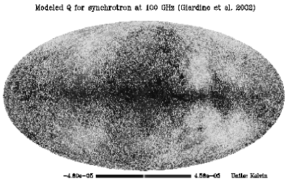
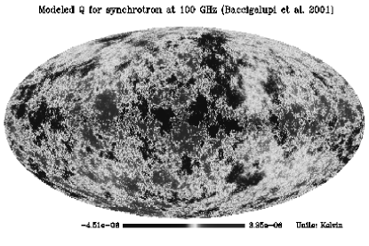
Figure 1: Q Stokes parameter for the emission of Galactic synchrotron according to Giardino et al. (2002, left panel) and Baccigalupi et al. (2001, right panel). The maps are in antenna temperature, at 100 GHz.

Giardino et al. (2002) built a full sky map of synchrotron polarized emission based on the total intensity map by Haslam et al. (1982), assuming a synchrotron polarized component at the theoretical maximum level of $75\%$, and a Gaussian distribution of polarization angles with a power spectrum estimated out of the high resolution radio band data (Duncan et al. 1997, 1999; Duncan et al. 1999). The polarization map obtained, reaching a resolution of about $10^{\prime}$, was then scaled to higher frequencies by considering either a constant or a space-varying spectral index as inferred by multi-frequency radio observations.

In this work we concentrate on low frequencies, modelling the diffuse polarized emission as a superposition of CMB and synchrotron. We used the synchrotron spatial template by Giardino et al. (2002), hereafter $S_{G}$ model, as well as another synchrotron template, hereafter indicated as $S_{B}$, obtained by scaling the spherical harmonics coefficients of the $S_{G}$ model to match the spectrum found by Baccigalupi et al. (2001). The $Q$ Stokes parameter for the two spatial templates, in antenna temperature at 100 GHz, are shown in Fig. 1, plotted in a non-linear scale to highlight the behavior at high Galactic latitudes. Note how the contribution on smaller angular scales is larger in the $S_{G}$ model. This is evident in Fig. 2 where we compare the power spectra of the $S_{G}$ and $S_{B}$ models with the CMB one, for the cosmological parameters of Eq. (1). Both models imply a severe contamination of the CMB $E$ mode on large angular scales, say $\ell\,\lower 2.0pt\hbox{${<\atop\hbox{\raise 4.0pt\hbox{$\sim$}}}$}\,200$, which remains serious even if the Galactic plane is cut out: cutting the region $|b|\leq 20^{\circ}$ decreases the $S_{G}$ and $S_{B}$ signals by about a factor of 10 and 3, respectively; the difference comes from the fact that the $S_{B}$ power is concentrated more on large angular scales, which propagate well beyond the Galactic plane (see Fig. 2).

In the $S_{G}$ case the contamination is severe also for the first CMB acoustic oscillation in polarization, as a result of the enhanced power on small angular scales with respect to the $S_{B}$ models (see also Fig. 1). On smaller scales both models predict the dominance of CMB $E$ modes. On the other hand, CMB $B$ modes are dominated by foreground emission, even if the region around the Galactic plane is cut out as we commented above.

To obtain the synchrotron emission at different frequencies, we consider either a constant antenna temperature spectral index of $-2.9$, slightly shallower than indicated by the WMAP first year measurements (Bennett et al. 2003b), as well as a varying spectral index. In Fig. 3 we show the map of synchrotron spectral indices, in antenna temperature, which we adopt following Giardino et al. (2002). Note that this aspect is relevant especially for component separation, since all methods developed so far require a “rigid” frequency scaling of all the components, which means that all components should have separable dependencies on sky direction and frequency. Actually this requirement is hardly satisfied by real signals, and by synchrotron in particular. However, as we see in the next Section, FastICA results turn out to be quite stable as this assumption is relaxed, at least for the level of variation in Fig. 3. This make this technique very promising for application to real data. A more quantitative study of how the FastICA performance gets degraded when realistic signals as well instrumental systematics are taken into account will be carried out in a future work.

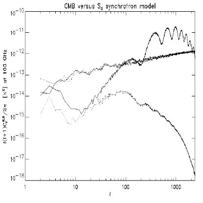
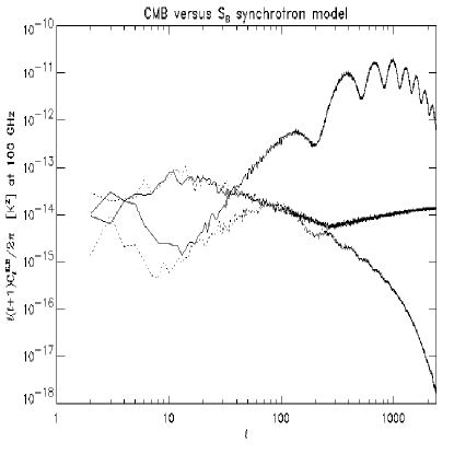
Figure 2: $E$ (solid) and $B$ (dotted) angular power spectra of CMB and synchrotron polarization emission, in antenna temperature, at 100 GHz, according to the $S_{G}$ (left panel), and $S_{B}$ (right panel) polarized synchrotron template.

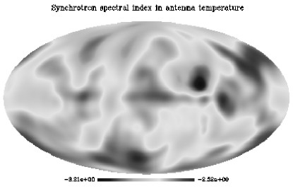
Figure 3: Map of synchrotron spectral indices (Giardino et al. 2002).

3 Component separation for polarized radiation

Component separation has been implemented so far for the total intensity signal (see Maino et al. 2002, Stolyarov et al. 2002, and references therein). In this Section we expose how we extend the ICA technique to treat polarization measurements.

3.1 $E$ and $B$ modes

As we stressed in the previous Section, the relevant information for the CMB polarized signal can be conveniently read in a non-local combination of $Q$ and $U$ Stokes parameters, represented by the $E$ and $B$ modes (see Zaldarriaga & Seljak 1997 and Kamionkowski, Kosowsky, & Stebbins 1997). There are conceptually two ways of performing component separation in polarization observations. $Q$ and $U$ can be treated separately, i.e. performing separation for each of them independently. However, in the hypothesis that $Q$ and $U$ have the same statistical properties, separation can be conveniently performed on a data-set combining $Q$ and $U$ maps. This is surely the appropriate strategy if one is sure that the choice of polarization axes of the instrumental set-up does not bias the signal distribution. In general, however, it may happen that accidentally the instrumental polarization axes are related to the preferred directions of the underlying signal, making $Q$ and $U$ statistically different, so that merging them in a single data-set would not be appropriate. While for the Gaussian CMB statistics we do not expect such occurrence, it may happen for foregrounds, expecially if separation is performed on sky patches. For example, the Galactic polarized signal possesses indeed large scale structures with preferred directions, such as the Galactic Plume, discovered by Duncan et al. (1998) in the radio band, extending up to 15 degrees across the sky and reaching high Galactic latitudes. Therefore, in general, the most conservative approach to component separation in polarization is to perform it for $Q$ and $U$ separately. Note that in our Galactic model no coherence in the polarization detection is present. This allow us to verify, in the next Section, that the results obtained by merging $Q$ and $U$ in a single data-set are quite equivalent or more accurate than those obtained by treating them separately. In the following we report the relevant FastICA formalism for the latter case. Otherwise, when $Q$ and $U$ form a single template, the same formulas developed in Maino et al. (2002) do apply.

Let these multi-frequency maps be represented by ${\bf x}^{Q}$ and ${\bf x}^{U}$ respectively, where ${\bf x}$ is made of two indexes, labelling frequencies on rows and pixel on columns. If the unknown components to be recovered from the input data scale rigidly in frequency, which means that each of them can be represented by a product of two functions depending on frequency and space separately, we can define a spatial pattern for them, which we indicate with ${\bf s}^{Q}$ and ${\bf s}^{U}$. Then we can express the inputs ${\bf x}^{Q,U}$ as

$${\bf x}^{Q,U}={\bf A}^{Q,U}{\bf B}\,{\bf s}^{Q,U}+{\bf n}^{Q,U}\ ,$$ (2)

where the matrix ${\bf A}^{Q,U}$ scales the spatial patterns of the unknown components to the input frequencies, thus having a number of rows equal to the number of input frequencies. The instrumental noise ${\bf n}$ has same dimensions as ${\bf x}$. The matrix B represents the beam smoothing operation: we recall that at the present level of architecture, an ICA based component separation requires to deal to maps having equal beams at all frequencies. Separation is achieved in the real space, by estimating two separation matrices, ${\bf W}^{Q}$ and ${\bf W}^{U}$, having a number of rows corresponding to the number of independent components and a number of columns equal to the frequency channels, which produce a copy of the independent components present in the input data:

$${\bf y}^{Q}={\bf W}^{Q}{\bf x}^{Q}\ \ ,\ \ {\bf y}^{U}={\bf W}^{U}{\bf x}^{U}\ .$$ (3)

All the details on the way the separation matrix for FastICA is estimated are given in Maino et al. (2002). ${\bf y}^{Q}$ and ${\bf y}^{U}$ can be combined together to get the $E$ and $B$ modes for the independent components present in the input data (see Zaldarriaga, Seljak 1997 and Kamionkowski, Kosowsky, Stebbins 1997). Note that failures in separation for even one of $Q$ and $U$ affect in general both $E$ and $B$, since each of them receive contributions from both $Q$ and $U$. It is possible, even in the noisy case, to check the quality of the resulting separation by looking at the product ${\bf W}{\bf A}$, which should be the identity in the best case. This means that the frequency scalings of the recovered components can be estimated: following Maino et al. (2002), by denoting as $x_{\nu\,j}^{Q,U}$ the $j$-th component in the data x at frequency $\nu$, it can be easily seen that the frequency scalings are simply the ratios of the column elements of the matrices W^-1:

$${x_{\nu\,j}^{Q,U}\over x_{\nu^{\prime}\,j}^{Q,U}}={({\rm\bf W}^{Q,U})^{-1}_{\nu\,j}\over({\rm\bf W}^{Q,U})^{-1}_{\nu^{\prime}\,j}}\ .$$ (4)

However, it is important to note that even if separation goes virtually perfect, which means that ${\bf W}{\bf A}$ is exactly the identity, Eqs. (2,3) imply that noise is transmitted to the FastICA outputs, even if it can be estimated and, to some extent, taken into account during the separation process.

3.2 Instrumental noise

Our method to deal with instrumental noise in a FastICA-based separation approach is described in Maino et al. (2002), for total intensity maps. Before starting the separation process, the noise correlation matrix, which for a Gaussian, uniformly distributed noise is null except for the noise variances at each frequency on the diagonal, is subtracted from the total signal correlation matrix; the “denoised” signal correlation matrix enters then as an input in the algorithm performing separation. The same is done also here, for $Q$ and $U$ separately. Moreover, in Maino et al. (2002) we described how to estimate the noise of the FastICA outputs. In a similar way, let us indicate the input noise patterns as ${\bf n}^{Q,U}$. Then from Eqs. (2,3) it can be easily seen that the noise on FastICA outputs is given by

$${\bf n}_{y}^{Q,U}={\bf W}^{Q,U}{\bf n}^{Q,U}\ ,$$ (5)

which means that, if the noises on different channels are uncorrelated, and indicating as $\sigma_{\nu_{j}}$ the input noise $rms$ at frequency $\nu_{j}$, the noise $rms$ on the $i$-th FastICA output is

$$\sigma_{y_{i}}^{Q,U}=\sqrt{\sum_{j}|W_{ij}^{Q,U}|^{2}|\sigma_{\nu_{j}}^{Q,U}|^{2}}\ .$$ (6)

Note that the above equation describes the amount of noise which is transmitted to the outputs after the separation matrix has been found, and not how much the separation matrix is affected by the noise. As treated in detail in Maino et al. (2002), if the noise correlation matrix is known, it is possible to subtract it from the signal correlation matrix, greatly reducing the influence of the noise on the estimation of ${\bf W}^{Q,U}$; however, sample variance and in general any systematics will make the separation matrix noisy in a way which is not accounted by Eq.(6).
On whole sky signals, the contamination to the angular power spectrum coming from a uniformly distributed, Gaussian noise characterized by $\sigma$ is $C_{\ell}=4\pi\sigma^{2}/N$, where $N$ is the pixel number on the sphere. The noise contamination to $C_{\ell}$s on $Q$ and $U$ can therefore be estimated easily on FastICA outputs once $\sigma_{\nu_{j}}^{Q,U}$ in Eq. (6) are known. Gaussianity and uniformity make also very easy to calculate the noise level on $E$ and $B$ modes, since they contribute at the same level. Thus we can estimate the noise contamination in the $E$ and $B$ channels as

$$C_{\ell\,y_{i}}^{E}=C_{\ell\,y_{i}}^{B}={C_{\ell\,y_{i}}^{Q}+C_{\ell\,y_{i}}^{U}\over 4}={\pi(|\sigma_{y_{i}}^{Q}|^{2}+|\sigma_{y_{i}}^{U}|^{2})\over N}\ ,$$ (7)

where the factor 4 is due to the normalization according to the HEALPix scheme (version 1.10 and less), featuring conventions of Kamionkowski, Kosowsky, & Stebbins (1997), whereas the other common version (Zaldarriaga & Seljak 1997) would yield a factor 2. The quantities defined in Eq. (7) represent the average noise power, which can be simply subtracted from the output power spectra by virtue of the uncorrelation between noise and signal; the noise contamination is then represented by the power of noise fluctuations around the mean [Eq. (7)]:

$$\Delta C_{\ell\,y_{i}}^{E}=\Delta C_{\ell\,y_{i}}^{B}=\sqrt{2\over 2\ell+1}\left[{\pi(|\sigma_{y_{i}}^{Q}|^{2}+|\sigma_{y_{i}}^{U}|^{2})\over N}\right]\ .$$ (8)

Note that the noise estimation is greatly simplified by our assumptions: a non-Gaussian and/or non-uniform noise, as well as a non-zero $Q/U$ noise correlation etc. could lead for instance to non-flat noise spectra for $C_{\ell}$s, as well as non-equal noises in $E$ and $B$ modes. However, if a good model of these effects is available, a Monte Carlo pipeline is still conceivable by calculating many realizations of noise to find the average contamination to $E$ and $B$ modes to be subtracted from outputs instead of the simple forms of Eqs. (7,8).

4 Performance study

In this Section we apply our approach to simulated skies to assess: $(i)$ the ultimate capability of FastICA to clean the CMB maps from synchrotron in ideal noise-less conditions, $(ii)$ how the results are degraded by noise.

4.1 Noiseless separation

We work with angular resolution of $3^{\prime}.5$, corresponding to $n_{side}=1024$ in an HEALPix environment (Górski et al. 1999); this is enough to test the performance of the CMB polarization reconstruction, in particular for the undamped sub-degree acoustic oscillations, extending up to $\ell\simeq 2000$ in Fig. 2. In all the cases we show, the computing time to achieve separation was of the order of a few minutes on a Pentium IV 1.8 GHz processor with 512 Mb RAM memory. We perform separation by considering the CMB model defined by Eq. (1) and both the $S_{G}$ (Giardino et al. 2002) and the $S_{B}$ (Baccigalupi et al. 2001) model for synchrotron emission. We have considered $Q$ and $U$ maps both separately and combined.

As we already mentioned, the FastICA performance turns out to be stable against relaxation of rigid frequency scalings, at least for the spectral index variations shown in Fig. 3. In order to illustrate quantitatively this point, we compare the quality of the CMB reconstruction assuming either constant and varying synchrotron spectral indices, $\beta$. In Fig. 4 we plot the original (dotted) and reconstructed (solid) $C_{\ell}^{E,B}$s for CMB, in the case of the $S_{B}$ foreground model with constant (left-hand panels) or spatially varying $\beta$. The upper (lower) panels refer to the two frequency combinations 70, 100 (30, 44) GHz channels. Figure 5 shows the results of the same analisys, but using the $S_{G}$ model.

As it can be seen, the CMB signal is well reconstructed on all relevant scales, down to the pixel size. The same is true for the synchrotron emission, not shown. Percent precision in frequency scaling recovery for CMB and synchrotron is achieved (see Table 1). As we stressed in the previous Section, the precision on frequency scaling recovery corresponds to the precision on the estimation of the elements in the inverse of the matrices ${\bf W}^{Q}$ and ${\bf W}^{U}$. Remarkably, FastICA is able to recover the CMB $B$ modes on all the relevant angular scales, even if they are largely subdominant with respect to the foreground emission, as it can be seen in Fig. 2. This is due to two main reasons: the difference of the underlying statistics describing the distribution of CMB and foreground emission, and the high angular resolution of templates ($3^{\prime}.5$). Such resolution allows the algorithm to converge close to the right solution by exploiting the wealth of statistical information contained in the maps. Note also that in the noiseless case with constant synchrotron spectral index, the CMB power spectrum is reconstructed at the same good level both for the 100, 70 GHz and for 30, 44 GHz channel combinations, although in this frequency range the synchrotron emission changes amplitude by a factor of about 10. Indeed, by comparing top and bottom left panels of Figs. 4 and 5, one can note that there is only a minimum difference between the $B$ spectra at 44 GHz and at 100 GHz, arising at high $\ell$, while the $E$ spectra exhibit no appreciable difference at all.

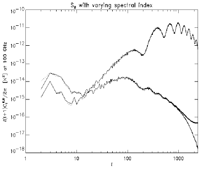
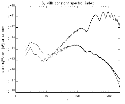
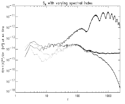
Figure 4: Original (dotted) and reconstructed (solid) power spectra for $E$ and $B$ CMB modes in the case of the $S_{B}$ model, in the absence of noise. Left panels: constant spectral index. Right panels: space varying spectral index. Upper panels are from inputs at 70 and 100 GHz channels, while bottom panels corresponds to inputs at 30 and 44 GHz. The outputs are conventionally plotted at the highest input frequency.

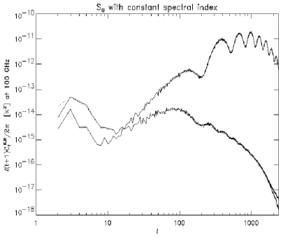
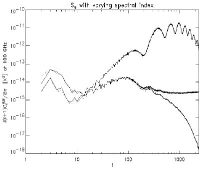
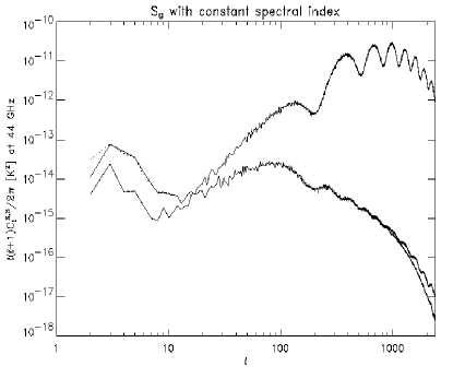
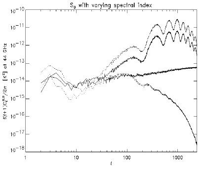
Figure 5: Original (dotted) and reconstructed (solid) power spectra for $E$ and $B$ CMB modes in the case of $S_{G}$ model, in the absence of noise. Left panels: constant spectral index. Right panels: space varying spectral index. Upper panels are from inputs at 70 and 100 GHz channels, while bottom panels corresponds to inputs at 30 and 44 GHz. The outputs are conventionally plotted at the highest input frequency

In the case of spatially varying spectral index (right-hand panels of Figs. 4 and 5) a rigorous component separation is virtually impossible, since the basic assumptions of rigid frequency scaling is badly violated. However FastICA is able to approach convergence by estimating a sort of “mean” foreground emission, scaling roughly with the mean value of the spectral index distribution. Some residual synchrotron contamination of the CMB reconstructed maps cannot be avoided, however. This residual is proportional to the difference between the “true” synchrotron emission and that corresponding to the “mean” spectral index and is thus less relevant at the higher frequencies, where synchrotron emission is weaker. As shown by the upper right-hand panels of Figs. 4 and 5, when the 70–100 GHz combination is used, the power spectrum of the CMB $E$-mode is still well reconstructed on all scales, and even that of the CMB $B$-mode is recovered at least up to $\ell\simeq 100$. On smaller scales synchrotron contamination of the $B$-mode is strong in the $S_{G}$, but not in the $S_{B}$ (at least up to $\ell\simeq 1000$) case. As expected, the separation quality degrades substantially if the 30–44 GHz combination is used (right-hand, bottom panels of Figs. 4 and 5; see also Table 1 where the quoted error on frequency scaling for varying spectral index is the percentage difference between the average values $<(\nu_{1}/\nu_{2})^{\beta}>$ computed on input and reconstructed synchrotron maps).

Table 1: Percentage errors on frequency scalings reconstruction in the noiseless case.

Synchrotron $S_{G}$ model	const. $\beta$		variable $\beta$
Frequencies used (GHz)	30, 44	70, 100	30, 44	70, 100
Q synch.	1.48 $\times 10^{-2}$	0.11	21.73	7.55
U synch.	5.71 $\times 10^{-3}$	4.56 $\times 10^{-2}$	21.73	7.55
Q CMB	0.31	2.69 $\times 10^{-2}$	207.36	1.18
U CMB	0.69	5.83 $\times 10^{-2}$	222.12	1.21
Synchrotron $S_{B}$ model	const. $\beta$		variable $\beta$
Frequencies used (GHz)	30, 44	70, 100	30, 44	70, 100
Q synch.	0.18	1.46	19.19	1.04
U synch.	0.137	1.10	19.73	1.04
Q CMB	1.01	8.79 $\times 10^{-2}$	6.15	9.62 $\times 10^{-2}$
U CMB	0.1448	1.24 $\times 10^{-2}$	9.028	0.107

To compare the FastICA performances when $Q$ and $U$ maps are dealt with separately or together (case $QU$), we have carried out a Monte Carlo chain on the CMB realizations, referring to the 70 and 100 GHz channels, and computed the $rms$ error on the CMB frequency scaling reconstruction, $\sigma_{Q}$, $\sigma_{U}$, and $\sigma_{QU}$. The results are shown in Table 2. Again the reconstruction is better when the weaker synchrotron model $S_{B}$ is considered. The slight difference between $\sigma_{Q}$ and $\sigma_{U}$ is probably due to the particular realization of the synchrotron model we have used (not changed through this Monte Carlo chain). The fact that the difference is present for both the $S_{B}$ and $S_{G}$ models is not surprising because the two models have different power as a function of angular scales but have the same distribution of polarization angles. The reason why we didn’t vary the foregrounds templates in our chain is the present poor knowledge of the underlying signal statistics.

The separation precision when $Q$ and $U$ are considered together is equivalent or better than if they are treated separately, as expected since the statistical information in the maps which are processed by FastICA is greater. On the other hand, the fact that $\sigma_{QU}$ is so close to $\sigma_{Q}$ and $\sigma_{U}$ clearly indicates that for a pixel size of about $3^{\prime}.5$ the statistical information in the maps is such that the results are not greatly improved if the pixel number is doubled. In the following we just consider the most general case in which $Q$ and $U$ maps are considered separately.

4.2 The effect of noise

To study the effect of the noise on FastICA component separation we use a map resolution of about $7^{\prime}$, corresponding to $n_{side}=512$ in an HEALPix scheme (Górski et al. 1999). At this resolution the all sky separation runs take a few seconds. Moreover we consider only the combination of 70 and 100 GHz channels, and a space varying synchrotron spectral index. We give the results for one particular noise realization and then we show that the quoted results are representative of the typical FastICA performance within the present assumptions. Moreover, we investigate how the foreground emission affects the recovered CMB map. The noise is assumed to be Gaussian and uniformly distributed, with $rms$ parameterized with the signal to noise ratio, $S/N$, where $S$ stays for CMB. As we already stressed, noise is either subtracted during the separation process, and on the reconstructed $C_{\ell}$, according to the estimate in Eq, (7). The results are affected by the residual noise fluctuations, with power given by Eq. (8).

Table 2: Percentage $rms$ for CMB frequency scaling reconstruction resulting from a Monte Carlo chain of FastICA applied to $50$ different CMB realizations at 70 and 100 GHz; $\sigma_{Q}$ and $\sigma_{U}$ are obtained by treating $Q$ and $U$ separately, while $\sigma_{QU}$ is the result when they are considered as a single array; the $1\sigma$ error on the parameter estimation, assuming Gaussianity, is also indicated.

	$\sigma_{Q}$	$\sigma_{U}$	$\sigma_{QU}$
Synchrotron $S_{G}$ model	$1.23\pm 0.17$	$1.17\pm 0.17$	$1.21\pm 0.17$
Synchrotron $S_{B}$ model	$0.104\pm 0.015$	$0.113\pm 0.016$	0$.102\pm 0.014$

As expected, the noise primarily affects the reconstruction of CMB $B$ mode. In Fig. 6 we plot the reconstructed and original CMB $E$- and $B$-mode power spectra, for $S_{G}$ (left) and $S_{B}$ (right) foreground emission, in the case $S/N=2$. With this level of noise, separation is still successful: the $E$-mode power spectrum comes out very well, while that of $B$-mode is well reconstructed up to the characteristic peak at $\ell\simeq 100$. Table 3 shows that the error on the frequency scaling recovery, for CMB, remains, in the noisy case, at the percent level both for $Q$ and $U$.

Figure 6: Original (dotted) and reconstructed (solid) 100 GHz power spectra for $E$ (top) and $B$ (bottom) CMB modes for the $S_{G}$ (left) and $S_{B}$ (right) cases, assuming $S/N$=2 and considering the 70 and 100 GHz channels; the synchrotron spectral index is space varying.

If the $S/N$ ratio is decreased, $B$ modes get quickly lost, while still the algorithm is successful in recovering the $E$ power spectrum for $S/N\,\lower 2.0pt\hbox{${>\atop\hbox{\raise 4.0pt\hbox{$\sim$}}}$}\,0.2$ (see Fig. 7). The algorithm starts failing at low multipoles, say $\ell\,\lower 2.0pt\hbox{${<\atop\hbox{\raise 4.0pt\hbox{$\sim$}}}$}\,100$, where synchrotron dominates over the CMB both in the $S_{G}$ and $S_{B}$ cases. The results in Fig. 7 for the $S_{G}$ case are averages over 8 multipoles, to avoid excessive oscillations of the recovered spectrum. For the $S/N$ ratios in this figure, the $B$-modes are lost on all scales. Since the $S_{G}$ model has a higher amplitude, FastICA is able to catch up the statistics more efficiently than for $S_{B}$, thus being able to work with a lower $S/N$ . Table 3 shows the degradation of the separation matrix for the $S/N$ ratios of Fig. 7, compared to the case with $S/N=2$.

Table 3: Percentage errors on CMB frequency scalings reconstruction in the noisy case by considering the 70 and 100 GHz channels.

Synchrotron $S_{G}$ model	$S/N=2$	$S/N=0.2$
Q CMB	1.04	13
U CMB	0.66	0.89
Synchrotron $S_{B}$ model	$S/N=2$	$S/N=0.5$
Q CMB	0.31	4.26
U CMB	0.34	0.35

We stress that the noise levels quoted here are not the maximum which the algorithm can support. The quality of the separation depends on the noise level as well as on the number of channels considered; adding more channels, while keeping constant the number of components to recover, generally improves the statistical sample with which FastICA deals and so the quality of the reconstruction as well as the amount of noise supported. In the next Section we show an example where a satisfactory separation can be obtained with higher noise by considering a combination of three frequency channels.

We now investigate to what extent the results quoted here are representative of the typical FastICA performance and study how the foreground emission biases the CMB maps recovered by FastICA. To this end we have performed a Monte Carlo chain of separation runs, building for each of them a map of residuals by subtracting the input CMB template from the recovered one and studying the ensemble of those residual maps.

The residuals in the noiseless case are just a copy of the foreground emission. Their amplitude is greatly reduced with respect to the true foreground amplitude, in proportion to the accuracy of the recovered separation matrix. Since the latter accuracy is at the level of percent of better, as it can be seen in Table 1, the residual foreground emission in the CMB recovered map is roughly the true one divided by 100. In terms of the angular power spectrum, see e.g. Fig. 2, the residual foreground contamination to the CMB recovered power spectrum is roughly a factor $10^{4}$ less than the true one.

In the of noisy separation a key feature is that at the present level of architecture, the FastICA outputs are just a linear combination of the input channels. Thus, even if the separation goes perfect, the noise is present in the output just as the same linear combination of the input noise templates. Note however that this does not mean that the noise is transmitted linearly to the outputs. The way the separation matrix is found depends non-linearly on the input data including the noise. In other words, the noise affects directly the estimation of the separation matrix, as we explained in Section 3.2. Eq. (6) describes only the amount of noise which affects the outputs after the separation matrix is found. As we shall see in a moment, at least in the case $S/N=2$ the main effect of the noise is the one given by Eq. (6), dominant over the error induced by the noise on the separation matrix estimation. Moreover, the noise in the outputs reflects the input noise statistics, which is Gaussian and uniformly dsitributed in the sky. As we shall see now, this is verified if the foreground contamination is the stronger $S_{G}$ one.

The results presented in Table 4 show the ensemble average of the mean of the residuals $<\bar{r}>$ together with its Gaussian expectation $<\bar{r}^{2}>_{G}^{1/2}$, and the mean $rms$ error on the CMB frequency scaling recovery, $\sigma$. The most important feature is that a non-zero mean value, at almost $10\sigma$ with respect to its Gaussian expectation, is detected. This is the only foreground contamination we find in the residuals. Note that the separation matrix precision recovery is at the percent level. That means that the present amount of noise does not affect significantly the accuracy of the separation process. Of course, if the noise is increased, the separation matrix estimation starts to be affected and eventually the foreground residual in the CMB reconstructed map will be relevant.

We made a further check by verifying that the residuals obey a Gaussian statistics with $rms$ given by Eq. 6 on all Galactic latitudes. We constructed a map having in each pixel the variance built out of the 50 residual maps in our Monte Carlo chain. In Fig. 8 we show the $rms$ of such map, plus/minus the standard deviation, calculated on rings with constant latitude with width equal to 1 degree. Together with the curves built out of our Monte Carlo chain, we report the theoretical values according to a Gaussian statistics, i.e. the average given by Eq. (6) equal to $(3.90\times 10^{-6}K)^{2}$, and the standard deviation over $N=50$ samples, given by $\sqrt{2(N-1)/N^{2}}\cdot(3.90\times 10^{-6}K)^{2}$. The agreement demonstrates that the Gaussian expectation is satisfied at all latitudes, expecially at the lowest, where the foreground contamination is expected to be maximum. Note that the fluctuations around the Gaussian theoretical levels are larger near the poles because of the enhanced sample variance.

We conclude that, within the present assumptions, for a successful separation the residual foreground contamination in the recovered CMB map is subdominant with respect to the noise. On the other hand, further tests are needed to check this result against a more realistic noise model, featuring the most important systematic effects like a non-uniform sky distribution, the presence of non-Gaussian features etc.

Figure 7: Input (dotted) and reconstructed (solid) 100 GHz power spectra for $E$ (top) and $B$ (bottom) CMB modes for the $S_{G}$ (left, assuming $S/N=0.2$, averaged over 8 multipole intervals) and $S_{B}$ (right, assuming $S/N=0.5$) cases, using the 70 and 100 GHz channels. The synchrotron spectral index is space varying.

5 An application to Planck

In this Section, we study how FastICA behaves in conditions corresponding to the instrumental capabilities of Planck. While this work was being completed, the polarization capabilities at 100 GHz were lost because of a funding problem of the Low Frequency Instrument (LFI), but that capability could be restored if the 100 GHz channel of the High Frequency Instrument (HFI) is upgraded, as it is presently under discussion. The Planck polarization sensitivity in all its channels has a crucial importance, and it is our intention to support this issue. Thus we work assuming Planck polarization sensitivity at 100 GHz, highlighting the fact that of our results have been obtained under this assumption. At 30, 44, 70 and 100 GHz, the Planck beams have full width half maximum (FWHM) of 33, 23, 14 and 10 arcmin, respectively. We study the FastICA effectiveness in recovering $E$, $B$ and $TE$ modes, separately. We adopted, for polarization, the nominal noise level for total intensity measurements increased by a factor $\sqrt{2}$ (note also that due to the 1.10 and lower HEALPix version convention to normalize $Q$ and $U$ following the prescription by Kamionkowski, Kosowsky and Stebbins 1997, a further $\sqrt{2}$ has to be taken into account when generating $Q$ and $U$ maps out of a given power in $E$ and $B$). We neglect all instrumental systematics in this work. The Planck instrumental features assumed here, with noise $rms$ in antenna temperature calculated for a pixel size of about 3.52 arcmin corresponding to $nside=1024$ in the HEALPix scheme, are summarized in Table 5. By looking at the numbers, it can be immediately realized that the level of noise is sensibly higher than the one considered in the previous Section, so that the same method would not work in this case and an improved analysis, involving more channels as described below, is necessary.

Table 4: Statistics of CMB residuals in Kelvin and percentage errors on frequency scaling reconstruction for the case $S_{G}$, $S/N=2$, 70 and 100 GHz channels, on 50 different noise and CMB realizations. The $1\sigma$ error on the parameter estimation, assuming Gaussianity, is also indicated.

Stokes parameter	$<\bar{r}>$	$<\bar{r}^{2}>_{G}^{1/2}$	$\sigma$
$Q$	$(3.94\pm 0.56)\cdot 10^{-8}$	$(2.20\pm 0.31)\cdot 10^{-9}$	$1.14\pm 0.16$
$U$	$(4.03\pm 0.57)\cdot 10^{-8}$	$(2.20\pm 0.31)\cdot 10^{-9}$	$0.74\pm 0.10$

Figure 8: Latitude analysis of the variance map calculated out of the residual maps in our Monte Carlo chain, in the case $S_{G}$, $S/N=2$, 70 and 100 GHz channels. The solid line is the average at the corresponding latitude, while the dashed curve represent the average plus/minus the standard deviation. The dotted lines are derived assuming Gaussian statistics.

Table 5: Planck-polarization performance assumed in this work.

Frequency (GHz, LFI)		30	44	70	100
FWHM (arcmin.)		33	23	14	10
noise $rms$ for $3.52^{\prime}$ pixels ($\mu$K)		80	81	69	52

5.1 $E$ mode

Due to the high noise level, we found convenient to include in the analysis the lower frequency channels together with those at 70 and 100 GHz. Since the FastICA algorithm is unable to deal with channels having different FWHM, as in Maino et al. (2002), we had to degrade the maps, containing both signal and noise, to the worst resolution in the channels considered. However, a satisfactory recovery of the CMB $E$ modes, extending on all scales up to the instrument best resolution, is still possible by making use of the different angular scale properties of both synchrotron and CMB. Indeed, as it can be seen in Fig. 2, the Galaxy is likely to be a substantial contaminant on low multipoles, say $\ell\,\lower 2.0pt\hbox{${<\atop\hbox{\raise 4.0pt\hbox{$\sim$}}}$}\,200$.

For the present application, we found convenient to use a combination of three Planck channels, 44, 70, 100 GHz for the $S_{G}$ and 30, 70, 100 GHz for the $S_{B}$ models, respectively. The reason of the difference is that the $S_{B}$ contamination is weaker, and the 30 GHz channel is necessary for FastICA to catch synchrotron with enough accuracy. Including a fourth channel does not imply relevant improvements. The maps, including signals properly smoothed and noise according to the Table 5, were simulated at $3.52^{\prime}$ resolution, corresponding to $n_{side}=1024$. Higher frequency maps were then smoothed to the FWHM of the lowest frequency channel and then re-gridded to $n_{side}=128$, corresponding to a pixel size of about $28^{\prime}$ and to a maximum multipole $\ell\simeq 400$. In all the cases shown, the spectral index for synchrotron has been considered variable. Fig. 9 shows the resulting CMB $E$ mode power spectrum after separation, for the $S_{G}$ (left) and $S_{B}$ (right) synchrotron models. An average every 4 (left) and 3 (right) coefficients was applied to eliminate fluctuations going negative on the lowest signal part at $\ell\simeq 10$. The agreement between the original spectrum and the reconstructed one is good on all the scales probed at the present resolution, up to $\ell\simeq 400$. The re-ionization bump is clearly visible as well as the first polarization acoustic oscillation at $\ell\simeq 100$. Moreover, there is no evident difference in the quality of the reconstruction between the two synchrotron models adopted.

Figure 9: Original (dotted) and reconstructed (solid) CMB $C_{\ell}^{E}$ obtained by applying the FastICA algorithm to the combination of 44, 70, and 100 GHz channels for the $S_{G}$ synchrotron case (left) and of 30, 70, and 100 GHz channels for the $S_{B}$ model (right).

Let us turn now to the degree and sub-degree angular scales, $\ell\,\lower 2.0pt\hbox{${>\atop\hbox{\raise 4.0pt\hbox{$\sim$}}}$}\,200$. As we already stressed, the Galaxy is expected to yield approximately equal power on $E$ and $B$ modes (see Fig. 2). On the other hand, CMB $E$ and $B$ modes are dramatically different on sub-degree angular scales. Summarizing, on $\ell\,\lower 2.0pt\hbox{${>\atop\hbox{\raise 4.0pt\hbox{$\sim$}}}$}\,200$, we expect to have

$$C_{\ell}^{E\,Gal}\simeq C_{\ell}^{B\,Gal}\ \ ,\ \ C_{\ell}^{E\,CMB}\gg C_{\ell}^{B\,CMB}\ .$$ (9)

Therefore, on $\ell\,\lower 2.0pt\hbox{${>\atop\hbox{\raise 4.0pt\hbox{$\sim$}}}$}\,200$ where the CMB contamination from synchrotron is expected to be irrelevant, the power spectrum of the CMB $E$ modes can be estimated by simply subtracting, together with the noise, the $B$ power as

$$C_{\ell}^{E\,CMB}\simeq C_{\ell}^{E\,CMB+Gal}-C_{\ell}^{B\,CMB+Gal}-C_{\ell}^{E\,noise}\ ,$$ (10)

where the total map CMB$+$Gal is used without any separation procedure. In other words, there is no need to perform separation to get the CMB $E$ modes at high multipoles, because they are simply obtained by subtracting the $B$ modes of the sky maps, since the latter are dominated by synchrotron which has almost equal power on $E$ and $B$ modes. Fig. 10 shows the results of this technique applied to the Planck-HFI 100 GHz channel, assumed to have polarization capabilities, for both the $S_{G}$ and $S_{B}$ synchrotron models. Residual fluctuations are higher in the $S_{G}$ case since the synchrotron contamination is stronger. In both cases, CMB $E$ modes are successfully recovered in the whole interval $100\,\lower 2.0pt\hbox{${<\atop\hbox{\raise 4.0pt\hbox{$\sim$}}}$}\,\ell\,\lower 2.0pt\hbox{${<\atop\hbox{\raise 4.0pt\hbox{$\sim$}}}$}\,1000$. It has also to be noted that the same subtraction technique would not help on the lower multipoles considered before, since in that case the foreground contamination is so strong that the tiny fluctuations making Galactic $E$ and $B$ modes different are likely to hide the CMB signal anyway.

Figure 10: Input (dotted) and reconstructed (solid) CMB $C_{\ell}^{E}$ obtained by subtracting the expected level of noise as well as the synchrotron contaminations $S_{G}$ (left) and $S_{B}$ (right) assumed to be matched by the $B$-mode map. The adopted instrumental capabilities are those of the Planck-HFI channel at 100 GHz, assumed to be polarization-sensitive.

Our results here can be summarized as follows: in the case of Planck capabilities, the FastICA technique makes it possible to remove substantially the foreground contamination in the regions in which that is expected to be relevant. Planck is likely to measure the CMB $E$ modes over all multipoles up to $\ell\simeq 1000$.

5.2 $B$ mode

In Fig. 11 the $B$-mode power spectrum after FastICA separation described in the previous section is shown for the $S_{G}$ (left) and $S_{B}$ (right) synchrotron models. An average over 13 multipoles has been applied to both cases in order to avoid fluctuations going negative. The reconstructed signal approaches the original one at very low multipoles, say $\ell\,\lower 2.0pt\hbox{${<\atop\hbox{\raise 4.0pt\hbox{$\sim$}}}$}\,5$. At higher multipoles, where the $B$ signal is generated by gravitational waves, the overall amplitude appears to be recovered, even if with major contaminations especially in the region where the signal is low, i.e. right between the re-ionization bump and the raise toward the peak at $\ell\simeq 100$. Needless to say, such contaminations are due to a residual foreground emission.

In the insets of Fig. 11 we show (data points) the recovered B-mode power spectrum in the range between $30\leq\ell\leq 120$, averaged over 20 multipoles, with error bars given by Eq. (8). Even if the contamination is substantial, especially for $\ell\geq 100$ and for the $S_{G}$ case, the results show a sign of the characteristic rise of the spectrum due to cosmological gravitational waves.

Concluding, our results indicate that the FastICA technique is able to remove substantially the foreground contamination of the $B$ mode, up to the peak at $\ell\,\lower 2.0pt\hbox{${<\atop\hbox{\raise 4.0pt\hbox{$\sim$}}}$}\,100$ if the tensor to scalar perturbation ratio is at least $30\%$.

Figure 11: Original (dotted) and reconstructed (solid) CMB $C_{\ell}^{B}$ obtained by applying the FastICA algorithm to the combination of Planck 44, 70, and 100 GHz channels for the $S_{G}$ synchrotron case (left) and to the combination of 30, 70, and 100 GHz channels for the $S_{B}$ model (right). The data points in the insets show the recovered $B$-mode power spectrum in the range $30\leq\ell\leq 120$ averaged over 20 multipoles; the error bars are given by Eq. (8).

5.3 $TE$ mode

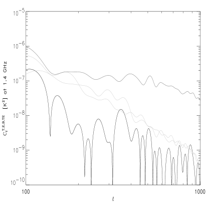
Figure 12: Power spectra of synchrotron $T$ (solid line),$E$ and $B$ (light lines), and $TE$ (heavy solid line) modes in the fan region at medium Galactic latitudes, at 1.4 GHz (Uyaniker et al. 1999).

While the cosmological $TE$ power spectrum is substantially stronger than that of any other polarized CMB mode, the opposite should happen in the case of foregrounds. On degree and sub-degree angular scales, a measure of the synchrotron $TE$ power spectrum can be achieved in the radio band. In the Parkes data at 1.4 GHz, Uyaniker et al. (1999) were able to isolate a region exhibiting pretty low rotation measures, named “fan region”, which is therefore expected to be only weakly affected by Faraday depolarization. This and other regions from the existing surveys in the radio band were used to predict the synchrotron power for the $S_{B}$ scenario (Baccigalupi et al. 2001).

In Fig. 12 we show the $T$, $E$, $B$, and $TE$ power spectra for the fan region. Total intensity anisotropies are represented by the upper curve (solid). $E$ and $B$ modes (light lines) have very similar behavior. The $TE$ mode (heavy solid line) is the weakest and, as it can be easily seen by scaling the $TE$ amplitude in Fig. 12 with the typical spectra index for synchrotron, it is markedly below the expected cosmological $TE$ signal at CMB frequencies. Both synchrotron models $S_{G}$ and $S_{B}$, are consistent with this result as illustrated by in Fig. 13. It is straightforward to check that our models for the synchrotron emission have a $TE$ power spectrum not far from the one in Fig. 12, when scaled to the appropriate frequency.

Figure 13: $C_{\ell}^{TE}$ of CMB (dotted) compared with that of synchrotron according to the $S_{G}$ (solid, left) and $S_{B}$ (solid, right) models, at 100 GHz.

From the point of view of CMB observations, this means that, if the synchrotron contamination at microwave frequencies is well represented by its signal in the radio band, at least on degree and sub-degree angular scales the contamination from synchrotron is almost absent due to the change in the magnetic field orientation along the line of sight. On the other hand, on larger scales, as it can be seen in Fig. 13, the contamination could be relevant both in the $S_{G}$ and $S_{B}$ cases and we perform component separation as described in Section 5.1 for the Planck case. In Fig. 14 we show the recovery of the CMB $TE$ mode, obtained by combining the templates of $Q$ and $U$ maps obtained after FastICA application as in Section 5.1, with the CMB $T$ template obtained, still with FastICA based component separation strategy, in Maino et al. (2002). Oscillations due to residual noise are visible in the recovered $C_{\ell}^{TE}$. However, as in the case of the $E$-mode, the procedure was successful in substantially removing the contamination.

Figure 14: $C_{\ell}^{TE}$ of original (dotted) and recovered (solid) CMB emission obtained with FastICA applied to simulated Planck maps, by considering the $S_{G}$ (left) and the $S_{B}$ (right) foreground model, respectively. Results are shown at 100 GHz.

Both in the $S_{G}$ and in the $S_{B}$ case the synchrotron contamination is almost absent in the acoustic oscillation region of the spectrum, as it is evident again from Fig. 13; neglecting it we get the results shown in Fig. 15. The combination of Planck angular resolution and sensitivity allows the recovery of the $TE$ power spectrum up to $\ell\simeq 1200$, corresponding roughly to the seventh CMB acoustic oscillation.

Figure 15: $C_{\ell}^{TE}$ of original (dotted) and recovered (solid) CMB emission adopting the $S_{G}$ (left) and the $S_{B}$ (right) synchrotron model, considering the Planck performances at 100 GHz.

6 Concluding remarks

Forthcoming experiments are expected to measure CMB polarization. The first detections have been obtained on pure polarization (Kovac et al. 2002), as well on its correlation with total intensity CMB anisotropies, by the Wilkinson Microwave Anisotropy Probe (WMAP) satellite.

The foreground contamination is mildly known for total intensity measurements, and poorly known for polarization (see De Zotti 2002 and references therein). It is therefore crucial to develop data analysis tools able to clean the polarized CMB signal from foreground emission by exploiting the minimum number of a priori assumptions. In this work, we implemented the Fast Independent Component Analysis technique in an astrophysical context (FastICA, see Amari, Chichocki 1998, Hyvärinen 1999, Baccigalupi et al. 2000, Maino et al. 2002) for blind component separation to deal with astrophysical polarized radiation.

In our scheme, component separation is performed both on the Stokes parameters $Q$ and $U$ maps independently and by joining them in a single dataset. $E$ and $B$ modes, coding CMB physical content in the most suitable way (see Zaldarriaga, Seljak 1997, Kamionkowski, Kosowsky, Stebbins 1997), are then built out of the separation outputs. We described how to estimate the noise on FastICA outputs, on $Q$ and $U$ as well as on $E$ and $B$.

We tested this strategy on simulated polarization microwave all sky maps containing a mixture of CMB and Galactic synchrotron. CMB is modelled close to the current best fit (Spergel et al. 2003), with a component of cosmological gravitational waves at the $30\%$ level with respect to density perturbations. We also included re-ionization, although with an optical depth lower than indicated by the WMAP results (Bennett et al. 2003a) since they came while this work was being completed, but consistent with the Gunn-Peterson measurements by Becker et al. (2001). Galactic synchrotron was modelled with the two existing templates by Giardino et al. (2002) and Baccigalupi et al. (2001). These models yield approximately equal power on angular scales above the degree, dominating over the expected CMB power. On sub-degree angular scales, the Giardino et al. (2002) model predicts an higher power, but still subdominant compared to the CMB $E$ mode acoustic oscillations. Note that at microwave frequencies, the fluctuations at high multipoles ($\ell\,\lower 2.0pt\hbox{${>\atop\hbox{\raise 4.0pt\hbox{$\sim$}}}$}\,1000$), corresponding to a few arcmin angular scales, are likely dominated by compact or flat spectrum radio sources (Baccigalupi et al. 2002b, Mesa et al. 2002). Their signal is included in the maps used to estimate the synchrotron power spectrum.

We studied in detail the limiting performance in the noiseless case, as well as the degradation induced by a Gaussian, uniformly distributed noise, by considering two frequency combinations: 30 $+$ 44 GHz and 70 $+$ 100 GHz. In the noiseless case, the algorithm is able to recover CMB $E$ and $B$ modes on all the relevant scales. In particular, this result is stable against the space variations of the synchrotron spectral index indicated by the existing data. In this case, FastICA is able to converge to an average synchrotron component, characterized by a “mean” spectral index across the sky, and to remove it efficiently from the map. The output CMB map, also containing residual synchrotron due to its space varying spectral index, is mostly good as far as the frequencies considered are those where the synchrotron contamination is weaker.

By switching on the noise we found that separation, at least for what concerns the CMB $E$ mode, is still satisfactory for noise exceeding the CMB but not the foreground emission. The reason is that in these conditions the algorithm is still able to catch and remove the synchrotron component efficiently. We implemented a Monte Carlo chain varying the CMB and the noise realizations in order to show that the performance quoted above is typical and does not depend on the particular case studied. Moreover, we studied how the foreground emission biases the recovered CMB map, by computing maps of residuals, i.e. subtracting the true CMB map out of the recovered one. In the noiseless case, the residual is just a copy of the foreground emission, with amplitude decreased proportionally to the accuracy of the separation matrix. In the noisy case, for interesting noise amplitudes the residual maps are dominated by the noise in the input data, linearly mixed with the separation matrix. The situation is obviously worse for the weaker CMB $B$ mode.

We applied these tools making reference to the Planck polarization capabilities, in terms of frequencies, angular resolution and noise, to provide a first example of how the FastICA technique could be relevant for high precision large polarization data-sets. We addressed separately the analysis of the CMB $E$, $B$, and $TE$ modes. While this work was being completed, the Low Frequency Instrument (LFI) lost its 100 GHz channel, having polarization sensitivity. However polarimetry at this frequency could be restored if the 100 GHz channel of the High Frequency Instrument (HFI) is upgraded, as is presently under discussion. Due to the scientific content of the CMB polarization signal, the Planck polarization sensitivity deserves a great attention. Within our context here, it is our intention to support the importance of having polarization capabilities in all the cosmological channels of Planck, and in particular at 100 GHz. Our results have been obtained under this assumption.

To improve the signal statistics, we found convenient to consider at least three frequency channels in the separation procedure, including the ones where the CMB is strongest, 70 and 100 GHz, plus one out of the two lower frequency channels, at 30 and 44 GHz. Since the latter have lower resolution we had to degrade the higher frequency maps since the present FastICA architecture cannot deal with maps having different resolutions. CMB $E$ and $TE$ modes were accurately recovered for both the synchrotron models considered. The $B$-mode power spectrum is recovered on very large angular scales in the presence of a conspicuous re-ionization bump. On smaller scales, where the $B$-mode power mainly comes from cosmological gravitational waves, the recovery is only marginal for a $30\%$ tensor to scalar perturbation ratio.

On the sub-degree angular scales the contamination from synchrotron is almost irrelevant according to both models (Giardino et al. 2002, Baccigalupi et al. 2001). Moreover, it is expected that Galactic $E$ and $B$ modes have approximately the same power (Zaldarriaga 2001), while for CMB the latter are severely damped down since they are associated with vector and tensor perturbations, vanishing on sub-horizon scales at decoupling corresponding to a degree or less in the sky (see Hu et al. 1999). This argument holds also if the $B$ mode power is enhanced by weak lensing effects from matter structures along the line of sight (see Hu 2002 and references therein). Therefore, on these scales, we expect the $E$ power spectrum to be a sum of Galactic and CMB contributions, while the $B$ power comes essentially from foregrounds only. In these conditions, the CMB $E$ power spectrum is recovered by simply subtracting the $B$ power spectrum.

We also estimated the $TE$ contamination from synchrotron to be irrelevant for CMB, because of the strength of the CMB $TE$ component due to the intrinsic correlation between scalar and quadrupole modes exciting $E$ polarization. By applying these considerations on sub-degree angular scales, as well as the results of the FastICA procedure described above on larger scales, we show how the Planck instrument is capable of recovering the CMB $E$ and $TE$ spectra on all scales down to the instrumental resolution, corresponding to a few arc-minutes scales. In terms of multipoles, the $E$ and $TE$ angular power spectra are recovered up to $1000$ and $1200$, respectively.

Summarizing, we found that the FastICA algorithm, when applied to a Planck-like experiment, could be able to substantially clean the foreground contamination on the relevant multipoles, corresponding to degree angular scales and above. Since the foreground contamination on sub-degree angular scales is expected to be subdominant, the CMB $TE$ and $E$ modes are recovered on all scales extending from the whole sky to a few arc-minutes. In particular, the FastICA algorithm can clean the $B$-mode power spectrum up to the peak due to primordial gravitational waves if the cosmological tensor amplitude is at least $30\%$ of the scalar one. In particular, we find that on large angular scales, of a degree and more, foreground contamination is expected to be severe and the known blind component separation techniques are able to efficiently clean the map from such contamination, as it is presently known or predicted.

Still, despite these good results, the main limitation of the present approach is the neglect of any instrumental systematics. While it is important to assess the performance of a given data analysis tool in the presence of the nominal instrumental features, as we do here, a crucial test is checking the stability of such tool with respect to relaxation of the assumptions regarding the most common sources of systematic errors, like beam asymmetry, non-uniform and/or non-Gaussian noise distribution etc., as well as the idealized behavior of the signals to recover. In this work we had a good hint about the second aspect, since we showed that FastICA is stable against relaxation of the assumption, common to all component separation algorithms developed so far, about the separability between space and frequency dependence for all the signal to recover. In a forthcoming work we will investigate how ICA based algorithms for blind component separation deal with maps affected by the most important systematics errors.

References

- [] Amari S., Chichocki A., 1998, Proc. IEEE 86, 2026
- [] Baccigalupi C., Bedini L., Burigana C., De Zotti G., Farusi A., Maino D., Maris M., Perrotta F., Salerno E., Toffolatti L., Tonazzini A., 2000, MNRAS, 318, 769
- [] Baccigalupi C., Burigana C., Perrotta F., De Zotti G., La Porta L., Maino D., Maris M., Paladini R., 2001, A&A, 372, 8
- [] Baccigalupi C., Balbi A., Matarrese S., Perrotta F., Vittorio N., 2002a, Phys.Rev. D65 063520
- [] Baccigalupi C., De Zotti G., Burigana C., Perrotta F., 2002b, in Astrophysical Polarized Backgrouds, AIP conference proc. 609, S. Cecchini, S. Cortiglioni, R. Sault, and C. Sbarra eds., p. 84
- [] Becker R.H. et al., 2001, AJ, 122, 2850
- [] Bennett C.L. et al., 2003a, ApJ, 583, 1
- [] Bennett C.L. et al., 2003b, ApJ in press, astro-ph/0302208 preprint available at lambda.gsfc.nasa.gov/
- [] Benoit A. et al. 2003, submitted to A & A, astro-ph/0306222
- [] Bernardi G., Carretti E., Cortiglioni S., Sault R.J., Kevsteven M.J., Poppi S., 2003, ApJ lett. in press, astro-ph/0307363
- [] Burigana C., La Porta L., 2002, in Astrophysical Polarized Backgrouds, AIP conference proc. 609, S. Cecchini, S. Cortiglioni, R. Sault, and C. Sbarra eds., p. 54
- [] Brouw W.N., Spoelstra T.A.T., 1976, A& AS 26, 129
- [] Bouchet F.R., Prunet S., Sethi S.K., 1999, MNRAS, 302, 663
- [] De Bernardis, P. et al., 2002, ApJ 564, 559
- [] De Zotti G., 2002 in Astrophysical Polarized Backgrouds, AIP conference proc. 609, S. Cecchini, S. Cortiglioni, R. Sault, and C. Sbarra eds., p. 295
- [] Duncan A.R., Haynes R.F., Jones K.L., Stewart R.T., 1997, MNRAS 291, 279
- [] Duncan A.R., Reich P., Reich W., Frst E., 1999, A& A 350, 447
- [] Duncan A.R., Haynes R.F., Reich W., Reich P., Grey A.D., 1998, MNRAS 299, 942
- [] Finkbeiner D.P. 2003, ApJS, 146, 407
- [] Finkbeiner D.P., Davis M., Schlegel D.J. 1999, Apj 524, 867
- [] Fosalba P., Lazarian A., Prunet S., Tauber J.A., 2002, in Astrophysical Polarized Backgrouds, AIP conference proc. 609, S. Cecchini, S. Cortiglioni, R. Sault, and C. Sbarra eds., p. 44
- [] Giardino G., Banday A.J., Górski K.M., Bennett K., Jonas J.L., Tauber J., 2002, A& A 387, 82
- [] see Górski K.M., Wandelt B.D., Hansen F.K., Hivon E., Banday A. J., 1999, astro-ph/9905275, and the HEALPix home page http://www.eso.org/science/healpix/
- [] Haffner L.M., Reynolds R.J., Tufte S.L., 1999, ApJ, 523, 223
- [] Halverson, N.W. et al. 2002, ApJ 568, 38
- [] Haslam C.G.T. et al., 1982, A&A S 47, 1
- [] Hyvärinen A., 1999, IEEE Signal Processing Lett. 6, 145
- [] Hobson M.P., Jones A.W., Lasenby A.N., Bouchet F., 1998, MNRAS 300, 1
- [] Hu W. 2002, Phys.Rev.D 65, 023003
- [] Hu W., Dodelson S., 2002, Ann.Rev.Astron.Astophys. 40, 171
- [] Hu W., White M., Seljak U., Zaldarriaga M., 1999, Phys.Rev. D57 3290
- [] Kamionkowski M., Kosowsky A., Stebbins A., 1997, Phys.Rev. D55, 7368
- [] Kodama H., Sasaki M., 1984, Progr. Theor. Phys. Suppl. 78, 1
- [] Komatsu E. et al., 2003, ApJ in press, astro-ph/0302223 preprint available at lambda.gsfc.nasa.gov/
- [] Kogut A. et al., 2003, ApJ in press, astro-ph/0302213 preprint available at lambda.gsfc.nasa.gov/
- [] Lazarian A., Prunet S., 2002, in Astrophysical Polarized Backgrouds, AIP conference proc. 609, S. Cecchini, S. Cortiglioni, R. Sault, and C. Sbarra eds., p. 32
- [] Kovac J. et al. 2002, Nature 420, 772
- [] Lee, A.T. et al. 2001, ApJ 506, 485
- [] Liddle A., Lyth D.H. 2000, Cosmological Inflation and Large Scale Structure, Cambridge University Press
- [] Maino D., Farusi A., Baccigalupi C., Perrotta F., Banday A. J., Bedini L., Burigana C., De Zotti G., Gòrski K. M., Salerno, E, 2002, MNRAS, 334, 53
- [] Maino D., Banday A.J., Baccigalupi C., Perrotta F., Gòrski K., 2003, submitted to MNRAS, astro-ph/0303657
- [] Mandolesi N., et al., 1998, Planck Low Frequency Instrument, a proposal submitted to ESA
- [] Mesa D., Baccigalupi C., De Zotti G., Gregorini L., Mack K.L., Vigotti M., Klein U., submitted to A& A, 2002
- [] Moscardini L., Bartelmann M., Matarrese S., Andreani P., MNRAS in press, 2002
- [] Padin S. et al., 2001, ApJL 549, L1
- [] Puget J. L., et al., 1998, High Frequency Instrument for the Planck mission, a proposal submitted to ESA
- [] Schlegel D.J., Finkbeiner D.P. & Davies M., 1998, ApJ 500, 525
- [] Seljak U., Zaldarriaga M., 1996, ApJ 469, 437
- [] Smoot G.F., 1999, in 3K cosmology, AIP conf. proc. 476, L. Maiani, F. Melchiorri, N. Vittorio eds, p. 1
- [] Spergel D.N. et al., 2003, ApJ in press, astro-ph/0302209, preprint available at lambda.gsfc.nasa.gov/
- [] Stolyarov V., Hobson M.P., Ashdown M.A.J., Lasenby A.N., 2002, MNRAS in press
- [] Tegmark M., Efstathiou G., 1996, MNRAS 281, 1297
- [] Tenorio L., Jaffe A. H., Hanany S., Lineweaver C.H., 1999, MNRAS 310, 823
- [] Toffolatti L., Argueso Gomez F., de Zotti G., Mazzei P., Franceschini A., Danese L., Burigana, C., 1998, MNRAS 297, 117
- [] Tucci M., Carretti E., Cecchini S., Fabbri R., Orsini M., Pierpaoli E., 2000, New Astronomy 5, 181
- [] Tucci M., Carretti E., Cecchini S., Nicastro L., Fabbri R., Gaensler B.M., Dickey J.M., McClure-Griffiths N.M., 2002, ApJ, 579, 607
- [] Uyaniker B., Frst E., Reich W., Reich P., Wielebinski R., 1999, A& AS 138, 31
- [] Vielva P., Martínez-Gonz’alez E., Cayón L., Diego J.M., Sanz J.L., Toffolatti L., 2001, MNRAS 326, 181
- [] Wright E.L., 1999, New Astr. Rev. 43, 257
- [] Zaldarriaga M., 2001, Phys.Rev.D 64, 103001
- [] Zaldarriaga M., Seljak U., 1997, Phys.Rev.D 55, 1830