Abstract

In this pedagogical lecture, I introduce some of the basic terminology and description of fluctuating fields as they occur on cosmology. I define various statistical, cosmological and sample homogeneity and explain what is meant by the fair sample hypothesis and cosmic variance. I illustrate these concepts using the simplest second-order statistics, i.e. the two–point correlation function and its Fourier transform the power-spectrum. I then give a brief overview of the properties of information relating to the properties of the phases of the Fourier modes of cosmological fluctuations which is not contained in these simpler statistics. Specifically, I explain how phase information of a particular form (called quadratic phase coupling) is encoded in the three–point correlation function (or, equivalently, the bispectrum).

1 Introduction

In most popular versions of the gravitational instability model for the origin of cosmic structure, particularly those involving cosmic inflation (Guth 1981; Guth & Pi 1982), the initial fluctuations that seeded the structure formation process form a Gaussian random field (Adler 1981; Bardeen et al. 1986). Gaussian random fields are the simplest fully-defined stochastic processes, which makes analysis of them relatively straightforward. Robust and powerful statistical descriptors can be constructed that have a firm mathematical underpinning and are relatively simple to implement. Second-order statistics such as the ubiquitous power-spectrum (e.g. Peacock & Dodds 1996) furnish a complete description of Gaussian fields. They have consequently yielded invaluable insights into the behaviour of large-scale structure in the latest generation of redshift surveys, such as the 2dFGRS (Percival et al. 2001). Important though these methods undoubtedly are, the era of precision cosmology we are now entering requires more thought to be given to methods for both detecting and exploiting departures from Gaussian behaviour.

The pressing need for statistics appropriate to the analysis of non-linear stochastic processes also suggests a need to revisit some of the fundamental properties cosmologists usually assume when studying samples of the Universe. Gaussian random fields have many useful properties. It is straightforward to impose constraints that result in statistically homogeneous fields, for example. Perhaps more relevantly one can understand the conditions under which averages over a single spatial domain are well-defined, the constraint of sample-homogeneity. The conditions under which such fields can be ergodic are also well established. It is known that smoothing Gaussian fields preserves Gaussianity, and so on. These properties are all somewhat related, but not identical. Indeed, looking at the corresponding properties of non-linear fields turns up some interesting results and delivers warnings to be careful. Exploring these properties is the first aim of this lecture.

Even if the primordial density fluctuations were indeed Gaussian, the later stages of gravitational clustering must induce some form of non-linearity. One particular way of looking at this issue is to study the behaviour of Fourier modes of the cosmological density field. If the hypothesis of primordial Gaussianity is correct then these modes began with random spatial phases. In the early stages of evolution, the plane-wave components of the density evolve independently like linear waves on the surface of deep water. As the structures grow in mass, they interact with other in non-linear ways, more like waves breaking in shallow water. These mode-mode interactions lead to the generation of coupled phases. While the Fourier phases of a Gaussian field contain no information (they are random), non-linearity generates non-random phases that contain much information about the spatial pattern of the fluctuations. Although the significance of phase information in cosmology is still not fully understood, there have been a number of attempts to gain quantitative insight into the behaviour of phases in gravitational systems. Ryden & Gramann (1991), Soda & Suto (1992) and Jain & Bertschinger (1998) concentrated on the evolution of phase shifts for individual modes using perturbation theory and numerical simulations. An alternative approach was adopted by Scherrer, Melott & Shandarin (1991), who developed a practical method for measuring the phase coupling in random fields that could be applied to real data. Most recently Chiang & Coles (2000), Coles & Chiang (2000), Chiang (2001) and Chiang, Naselsky & Coles (2002) have explored the evolution of phase information in some detail.

Despite this recent progress, there is still no clear understanding of how the behaviour of the Fourier phases manifests itself in more orthodox statistical descriptors. In particular there is much interest in the usefulness of the simplest possible generalisation of the (second-order) power-spectrum, i.e. the (third-order) bispectrum (Peebles 1980; Scoccimarro et al. 1998; Scoccimarro, Couchman & Frieman 1999; Verde et al. 2000; Verde et al. 2001; Verde et al. 2002). Since the bispectrum is identically zero for a Gaussian random field, it is generally accepted that the bispectrum encodes some form of phase information but it has never been elucidated exactly what form of correlation it measures. Further possible generalisations of the bispectrum are usually called polyspectra; they include the (fourth-order) trispectrum (Verde & Heavens 2001) or a related but simpler statistic called the second-spectrum (Stirling & Peacock 1996). Exploring the connection between polyspectra and non-linearly induced phase association is the second aim of this lecture.

The plan is as follows. In the following section I introduce some fundamental concepts underlying statistical cosmology, more-or-less from first principles. I do this in order to allow the reader to see explicitly what assumptions underlie standard statistical practise. In Section 3 I look at some of the contexts in which quadratic non-linearity may arise, either primordially or during the non-linear growth of structure from Gaussian fields. In Section 4 I revisit some of the basic properties used in Section 2 from the viewpoint of a particularly simple form of non-linearity, known as quadratic non-linearity, and show how some basic implicit assumptions may be violated. I then, in Section 5, explore how phase correlations arise in quadratic fields and relate these to higher-order statistics of quadratic fields.

2 Basic Statistical Concepts

I start by giving some general definitions of concepts which I will later use in relation to the particular case of cosmological density fields. In order to put our results in a clear context, I develop the basic statistical description of cosmological density fields; see also, e.g., Peebles (1980) and Coles & Lucchin (2002).

2.1 Fourier Description

I follow standard practice and consider a region of the Universe having volume $V_{u}$, for convenience assumed to be a cube of side $L\gg l_{s}$, where $l_{s}$ is the maximum scale at which there is significant structure due to the perturbations. The region $V_{u}$ can be thought of as a “fair sample” of the Universe if this is the case. It is possible to construct, formally, a “realisation” of the Universe by dividing it into cells of volume $V_{u}$ with periodic boundary conditions at the faces of each cube. This device is often convenient, but in any case one often takes the limit $V_{u}\rightarrow\infty$. Let us denote by $\bar{\rho}$ the mean density in a volume $V_{u}$ and take $\rho({\bf x})$ to be the density at a point in this region specified by the position vector ${\bf x}$ with respect to some arbitrary origin. As usual, the fluctuation is defined to be

$$\delta({\bf x})=[\rho({\bf x})-\bar{\rho}]/\bar{\rho}.$$ (1)

We assume this to be expressible as a Fourier series:

$$\delta({\bf x})=\sum_{{\bf k}}\ \delta_{{\bf k}}\ \exp(i{\bf k}\cdot{\bf x})=\sum_{\bf k}\ \delta^{*}_{\bf k}\ \exp(-i{\bf k}\cdot{\bf x});$$ (2)

the appropriate inverse relationship is of the form

$$\delta_{\bf k}={1\over V_{u}}\int_{V_{u}}\ \delta({\bf x})\exp(-i{\bf k}\cdot{\bf x})d{\bf x}.$$ (3)

The Fourier coefficients $\delta_{\bf k}$ are complex quantities,

$$\delta_{\bf k}=|\delta_{\bf k}|\exp{(i\phi_{\bf k})}$$ (4)

with amplitude $|\delta_{\bf k}|$ and phase $\phi_{\bf k}$. The assumption of periodic boundaries results in a discrete ${\bf k}$-space representation; the sum is taken from the Nyquist frequency $k_{\rm Ny}=2\pi/L$, where $V_{u}=L^{3}$, to infinity. Note that as $L\rightarrow\infty$, $k_{\rm Ny}\rightarrow 0$. Conservation of mass in $V_{u}$ implies $\delta_{{\bf k}=0}=0$ and the reality of $\delta({\bf x})$ requires $\delta_{\bf k}^{*}=\delta_{-{\bf k}}$.

If, instead of the volume $V_{u}$, we had chosen a different volume $V^{\prime}_{u}$ the perturbation within the new volume would again be represented by a series of the form (2), but with different coefficients $\delta_{\bf k}$. Now consider a (large) number $N$ of realisations of our periodic volume and label these realisations by $V_{u1}$, $V_{u2}$, $V_{u3}$, …, $V_{uN}$. It is meaningful to consider the probability distribution ${\cal P}(\delta_{\bf k})$ of the relevant coefficients $\delta_{\bf k}$ from realisation to realisation across this ensemble. One typically assumes that the distribution is statistically homogeneous and isotropic, in order to satisfy the Cosmological Principle, and that the real and imaginary parts of $\delta_{\bf k}$ have a Gaussian distribution and are mutually independent, so that

$${\cal P}(w)={V_{u}^{1/2}\over(2\pi\alpha^{2}_{k})^{1/2}}\exp\Bigl{(}-{w^{2}V_{u}\over 2\alpha^{2}_{k}}\Bigr{)},$$ (5)

where $w$ stands for either ${\rm Re}~{}[\delta_{\bf k}]$ or ${\rm Im}~{}[\delta_{\bf k}]$ and $\alpha_{k}^{2}=\sigma^{2}_{k}/2$; $\sigma_{k}^{2}$ is the spectrum. This is the same as the assumption that the phases $\phi_{\bf k}$ in equation (5) are mutually independent and randomly distributed over the interval between $\phi=0$ and $\phi=2\pi$. In this case the moduli of the Fourier amplitudes have a Rayleigh distribution:

$${\cal P}(|\delta_{\bf k}|,\phi_{\bf k})d|\delta_{\bf k}|d\phi_{\bf k}={|\delta_{\bf k}|V_{u}\over 2\pi\sigma^{2}_{k}}\exp\Bigl{(}-{|\delta_{\bf k}|^{2}V_{u}\over 2\sigma_{k}^{2}}\Bigr{)}d|\delta_{\bf k}|d\phi_{\bf k}.$$ (6)

Because of the assumption of statistical homogeneity and isotropy, the quantity ${\cal P}(\delta_{\bf k})$ depends only on the modulus of the wavevector ${\bf k}$ and not on its direction. It is fairly simple to show that, if the Fourier quantities $|\delta_{\bf k}|$ have the Rayleigh distribution, then the probability distribution ${\cal P}(\delta)$ of $\delta=\delta({\bf x})$ in real space is Gaussian, so that:

$${\cal P}(\delta)d\delta={1\over(2\pi\sigma^{2})^{1/2}}\exp\Bigl{(}-{\delta^{2}\over 2\sigma^{2}}\Bigr{)}d\delta,$$ (7)

where $\sigma^{2}$ is the variance of the density field $\delta({\bf x})$. This is a strict definition of Gaussianity. However, Gaussian statistics do not always require the distribution (7) for the Fourier component amplitudes. According to its Fourier expansion, $\delta({\bf x})$ is simply a sum over a large number of Fourier modes whose amplitudes are drawn from some distribution. If the phases of each of these modes are random, then the Central Limit Theorem will guarantee that the resulting superposition will be close to a Gaussian if the number of modes is large and the distribution of amplitudes has finite variance. Such fields are called weakly Gaussian.

2.2 Covariance Functions & Probability Densities

I now discuss the real-space statistical properties of spatial perturbations in $\rho$. The covariance function is defined in terms of the density fluctuation by

$$\xi({\bf r})={\langle[\rho({\bf x})-\bar{\rho}][\rho({\bf x}+{\bf r})-\bar{\rho}]\rangle\over\bar{\rho}^{2}}=\langle\delta({\bf x})\delta({\bf x}+{\bf r})\rangle.$$ (8)

The angle brackets in this expression indicate two levels of averaging: first a volume average over a representative patch of the universe and second an average over different patches within the ensemble, in the manner of §2.1. Applying the Fourier machinery to equation (8) one arrives at the Wiener–Khintchin theorem, relating the covariance to the spectral density function or power spectrum, $P(k)$:

$$\xi({\bf r})=\sum_{\bf k}\langle|\delta_{\bf k}|^{2}\rangle\exp(-i{\bf k}\cdot{\bf r}),$$ (9)

which, in passing to the limit $V_{u}\rightarrow\infty$, becomes

$$\xi({\bf r})={1\over(2\pi)^{3}}\int P(k)\exp(-i{\bf k}\cdot{\bf r})d{\bf k}.$$ (10)

Averaging equation (9) over ${\bf r}$ gives

$$\langle\xi({\bf r})\rangle_{{\bf r}}={1\over V_{u}}\sum_{\bf k}\langle|\delta_{\bf k}|^{2}\rangle\int\exp(-i{\bf k}\cdot{\bf r})d{\bf r}=0.$$ (11)

The function $\xi({\bf r})$ is the two–point covariance function. In an analogous manner it is possible to define spatial covariance functions for $N>2$ points. For example, the three–point covariance function is

$$\zeta(r,s)={\langle[\rho({\bf x})-\bar{\rho}][\rho({\bf x}+{\bf r})-\bar{\rho}][\rho({\bf x}+{\bf s})-\bar{\rho}]\rangle\over\bar{\rho}^{3}}$$ (12)

which gives

$$\zeta({\bf r},{\bf s})=\langle\delta({\bf x})\delta({\bf x}+{\bf r})\delta({\bf x}+{\bf s})\rangle,$$ (13)

where the spatial average is taken over all the points ${\bf x}$ and over all directions of ${\bf r}$ and ${\bf s}$ such that $|{\bf r}-{\bf s}|=t$: in other words, over all points defining a triangle with sides $r$, $s$ and $t$. The generalisation of (12) to $N>3$ is obvious.

The covariance functions are related to the moments of the probability distributions of $\delta({\bf x})$. If the fluctuations form a Gaussian random field then the N-variate distributions of the set $\delta_{i}\equiv\delta({\bf x}_{i})$ are just multivariate Gaussians of the form

$${\cal P}_{N}(\delta_{1},...,\delta_{N})={1\over{(2\pi)^{N/2}({\rm det}~{}C)^{1/2}}}\exp\Bigl{(}-{1\over 2}\sum_{i,j}\delta_{i}~{}C_{ij}^{-1}~{}\delta_{j}\Bigr{)}.$$ (14)

The correlation matrix $C_{ij}$ can be expressed in terms of the covariance function

$$C_{ij}=\langle\delta_{i}\delta_{j}\rangle=\xi({\bf r}_{ij}).$$ (15)

It is convenient to go a stage further and define the N-point connected covariance functions as the part of the average $\langle\delta_{i}...\delta_{N}\rangle$ that is not expressible in terms of lower order functions e.g.

$$\langle\delta_{1}\delta_{2}\delta_{3}\rangle=\langle\delta_{1}\rangle_{c}\langle\delta_{2}\delta_{3}\rangle_{c}+\langle\delta_{2}\rangle_{c}\langle\delta_{1}\delta_{3}\rangle_{c}+\langle\delta_{3}\rangle_{c}\langle\delta_{1}\delta_{2}\rangle_{c}+\langle\delta_{1}\rangle_{c}\langle\delta_{2}\rangle_{c}\langle\delta_{3}\rangle_{c}+\langle\delta_{1}\delta_{2}\delta_{3}\rangle_{c},$$ (16)

where the connected parts are $\langle\delta_{1}\delta_{2}\delta_{3}\rangle_{c}$, $\langle\delta_{1}\delta_{2}\rangle_{c}$, etc. Since $\langle\delta\rangle=0$ by construction, $\langle\delta_{1}\rangle_{c}=\langle\delta_{1}\rangle=0$. Moreover, $\langle\delta_{1}\delta_{2}\rangle_{c}=\langle\delta_{1}\delta_{2}\rangle$ and $\langle\delta_{1}\delta_{2}\delta_{3}\rangle_{c}=\langle\delta_{1}\delta_{2}\delta_{3}\rangle$. The second and third order connected parts are simply the same as the covariance functions. Fourth and higher order quantities are different, however. The connected functions are just the multivariate generalisation of the cumulants $\kappa_{N}$ (Kendall & Stewart 1977). One of the most important properties of Gaussian fields is that all of their N-point connected covariances are zero beyond N=2, so that their statistical properties are fixed once the set of two–point covariances (15) is determined. All large-scale statistical properties are therefore determined by the asymptotic behaviour of $\xi(r)$ as $r\rightarrow\infty$. This simplifying property is not shared by non–Gaussian fields, a fact we shall explore in Section 4.

3 Quadratic Non-Linearity

In this section I discuss some of the circumstances wherein quadratic non-linearity may arise. At the outset I should admit that this study is primarily phenomenological and our intention is largely to use this as a model that displays some consequences of non-linearity.

3.1 Phenomenology

As far as I am aware, the first application of quadratic density fields in a cosmological setting was in Coles & Barrow (1987) who were studying the possible sample properties of non-Gaussian temperature fluctuations on the cosmic microwave background sky. They in fact studied a series of models called $\chi_{n}^{2}$ models obtained via the transformation

$$Y=X_{1}^{2}+X_{2}^{2}+\ldots X_{n}^{2},$$ (17)

where $n$ is the order and the $X_{i}$ are independent Gaussian random fields with identical covariance functions. Similar models were also explored by Moscardini et al. (1991) using $Y$ to model either the primordial density field or the primordial gravitation potential; see also (Koyoma, Soda & Taruya 1999; Verde et al. 2000; Matarrese, Verde & Jimenez 2000; Verde et al. 2001; Komatsu & Spergel 2001). The case $n=1$ is the quadratic model of the present paper. There was no physical motivation for this as a model of CMB temperature fluctuations; it was used simply because one could calculate analytic results for such a field to compare with similar results for a Gaussian. Indeed the $\chi_{n}^{2}$ random field has been used as a model for non-Gaussian phenomena in a wide range of fields, including surface physics and geology (e.g. Adler 1981).

3.2 Inflation

Since the early 1980s (e.g. Guth & Pi 1982) it has been commonly believed that the inflationary scenario of the very early Universe results in the imprint of primordial Gaussian fluctuations. Since then, and with the invention of increasingly complicated models of the inflationary process, it has become clearer that inflation can produce significant levels of non-Gaussianity. The simplest “slow-roll” models of inflation involving a single dominant scalar field do indeed produce Gaussian fluctuations, but including non-linear terms and back-reaction does produce some element of non-Gaussianity as do extra degrees of freedom (Salopek & Bond 1990; Salopek 1992; Falk, Rangarajan & Srednicki 1993; Gangui et al. 1994; Wang & Kamionkowski 2000; Bartolo, Matarrese & Riotto 2002).

Typically the non-linear contributions arising during inflation manifest themselves as higher-order contributions to the effective Newtonian gravitational potential, $\Phi$ i.e.

$$\Phi=\phi+\alpha(\phi^{2}-\langle\phi^{2}\rangle)+\ldots,$$ (18)

where $\phi$ is a Gaussian field (not the phase) and $\alpha$ is a constant which is vanishingly small in most models. The term in $\langle\phi^{2}\rangle$ is needed to ensure $\Phi$ has zero mean. Since the mean value of the Newtonian potential is not physically meaningful anyway this term is not really important. A more radical suggestion for an inflation-induced quadratic model is offered by Peebles (1999a,b). In this model the density field is given by

$$\rho({\bf x})=\frac{1}{2}m^{2}\psi({\bf x})^{2},$$ (19)

where $\psi$ is a scalar field and $m$ is an effective mass. I return to the statistical consequences of this particular model in Section 5.

3.3 Gravitational Non-linearity

In a simple perturbative model, the non-linear density contrast at a point ${\bf r}$ can be modelled by the relation

$$\delta({\bf x})=\delta_{1}({\bf x})+\epsilon\delta_{2}({\bf x})$$ (20)

where $\delta_{1}({\bf x})$ is a Gaussian random field, $\delta_{2}({\bf x})$ is a quadratic random field derived by squaring $\delta_{1}$ and $\epsilon$ is a small factor that controls the degree of non-linearity. To be precise I should also include a constant term in this expression in order to ensure that $\langle\delta({\bf x})\rangle=0$, but this does not play any role in the following for reasons mentioned above so I ignore it. Using a constant $\epsilon$ is not rigorous but at least qualitatively it shows how the lowest non-linear corrections come into play. For a detailed discussion of perturbation theory done properly see Bernardeau et al. (2002).

3.4 Bias

Attempts to confront theories of cosmological structure formation with observations of galaxy clustering are complicated by the uncertain and possibly biased relationship between galaxies and the distribution of gravitating matter. A particular simple and useful way of modelling this relationship is through the idea of a local bias. In such models, the propensity of a galaxy to form at a point where the total (local) density of matter is $\rho$ is taken to be some function $f(\rho)$ (Coles 1993; Fry & Gaztanaga 1993). This boils down to a statement of the form

$$\delta_{g}({\bf x})=f[\delta({\bf x})],$$ (21)

where $\delta_{g}$ is the density contrast inferred from galaxy counts or other clustering statistics. In the simplest local bias models, $f(\delta)$ is a constant usually called $b$. Clearly a linear bias of this form simply scales the variance, covariance functions and power-spectra of the underlying field but has no effect on the detailed form of the statistical distribution. Models where the bias is non-linear (but still local) are useful as they subject constraints on the effect that the bias may have on galaxy clustering statistics, without making any particular assumption about the form of $f$ (Coles 1993). Fry & Gaztanaga (1993) discussed the implications of bias with the form

$$f(\delta)=\sum_{n=0}^{\infty}b_{n}\delta^{n},$$ (22)

in which the $b_{n}$ cannot all be chosen independently because the mean of $\delta_{g}$ must again be zero. On scale where the density field is linear, one can therefore see that a non-linear bias with $b_{2}\neq 0$ will result in quadratic contributions to $\delta_{g}$ even if they do not contribute significantly to $\delta$.

4 Asymptotic Properties

In developing the statistical background in Section 2, especially the Fourier description of random fluctuating fields, I made a number of assumptions along the way that were necessary in order for the resulting descriptors to be well-defined. The terminology relating to these assumptions is often used very loosely in cosmology, at least partly because they bear a relatively simple relationship to each other under when the fields one is dealing with are Gaussian. However, in the general case of non-Gaussian fields many subtleties arise relating to the presence of higher-order statistical correlations. It is especially important in the current era of high-precision developments in statistical cosmology also to be precise about the foundations.

In the following I discuss some of the large-scale properties of random fields in a formal fashion, with particular reference to the quadratic model. The behaviour of covariance functions on large-scales will turn out to be very important so, to take the simplest example, consider the Peebles model from Section 3.2. In this case we basically have a quadratic density field $\delta=\psi^{2}-<\psi^{2}>$ where $\psi$ is assumed to be a statistically homogeneous random field and I have subtracted the mean value of $\psi^{2}$ to ensure that $\delta$ has zero mean.

Let us suppose that $\psi$ has a well-behaved covariance function $\Gamma({\bf r})$ and that the covariance function of $\delta$ is, as usual, $\xi({\bf r})$. It is trivial to show that that

$$\xi({\bf r})=2\Gamma^{2}({\bf r})$$ (23)

so that $\xi({\bf r})$ must be positive for all ${\bf r}$ (Adler 1981). Note that adding constant terms to $\delta$ would not alter this behaviour. In the more general case of a field of the form $\delta=\psi+\alpha\psi^{2}$, such as the examples given in equations (16) & (18), the resulting covariance function has a behaviour of the form

$$\xi({\bf r})=\Gamma({\bf r})+\alpha^{2}\Gamma^{2}({\bf r}).$$ (24)

In this case the covariance function of the resulting field would contain terms of order $\Gamma({\bf r})$, the corresponding covariance function of the underlying Gaussian field. If $\Gamma({\bf r})<0$ on some scale then as long as $\alpha$ is small, the resulting $\xi({\bf r})$ need not be positive in this case.

4.1 Statistical Homogeneity

The formal definition of strict statistical homogeneity for a random field (also called stationarity) is that the set of finite-dimensional joint probability distributions, which I called ${\cal P}_{N}(\delta_{1},...,\delta_{N})$ in Section 2.3, must be invariant under spatial translations, i.e.

$${\cal P}_{N}(\delta({\bf x}_{1}),...,\delta({\bf x}_{N}))={\cal P}_{N}(\delta({\bf x}_{1}+{\bf x}),...,\delta({\bf x}_{N}+{\bf x}))$$ (25)

for any ${\bf x}$. This must be true for all orders $N$. For a Gaussian random field in which the form of ${\cal P}_{N}(\delta_{1},...,\delta_{N})$ is given by equation (23), necessary and sufficient conditions for $\delta({\bf x})$ to be strictly homogeneous is that the covariance function $\langle\delta({\bf x}_{1})\delta({\bf x}_{2})\rangle$ is a function of ${\bf x}_{1}-{\bf x}_{2}$ only (Adler 1981). Statistical isotropy can be added by requiring rotation-invariance. One can define weaker versions of homogeneity and isotropy according to which only the moments of the distribution be translation invariant. For example, second-order homogeneity and isotropy (all that is required for the analysis of power-spectra or two-point covariance functions) basically means that the function $\xi({\bf r})$ does not depend on either the origin or the direction of ${\bf r}$, but only on its modulus. Since the properties of a Gaussian random field depend only on second-order properties, this weaker condition is sufficient to require condition (25) in this case.

This does not mean that any function satisfying translation and rotation invariance is necessarily the covariance function of a homogeneous random field (in either the strict or second-order sense). For one thing the power spectrum must be positive (or zero) for all $k$, which places a constraint on the shape of any possible $\xi({\bf r})$ – which must be convex. The result (16) also implies that

$$\lim_{r\rightarrow\infty}{1\over r^{3}}\int_{0}^{r}\xi(r^{\prime})r^{\prime 2}dr^{\prime}=0$$ (26)

for such fields. A perfectly homogeneous distribution would have $P(k)\equiv 0$ and $\xi(r)$ would be identically zero for all $r$. Note, however, that it is possible for fields obeying either (23) or (24) to be statistically homogeneous.

4.2 Sample Homogeneity

Statistical homogeneity plays a vital role in both the analysis of clustering and the formal development of the theory of cosmological perturbation growth. Unfortunately the use of the word “homogeneity” in this context leads to a confusion regarding the more fundamental use of this word in cosmology. Standard cosmologies are based on the Cosmological Principle, which requires our Universe to be homogeneous and isotropic on large scales. More loosely, it needs to be sufficiently homogeneous and isotropic that the Robertson-Walker metric and the Friedmann equations furnish an adequate approximation to the evolution of the Universe. Statistical homogeneity as described above is a much weaker requirement than the requirement that one realisation from a probability ensemble (our Universe) has asymptotically small fluctuations when smoothed on a sufficiently large scale. In fact, the analogous relation to (26) in the case of sample homogeneity is far stronger:

$$\lim_{r\rightarrow\infty}\int_{0}^{r}\xi(r^{\prime})r^{\prime 2}dr^{\prime}=0$$ (27)

as this requires the real fluctuations in density to be asymptotically small within a single realisation. Notice that the requirement for sample homogeneity is such that in general the covariance function must change sign, from positive at the origin, where $\xi(0)=\sigma^{2}\geq 0$, to negative at some $r$ to make the overall integral (26) converge in the correct way.

It is clear from this discussion that statistical homogeneity does not require sample homogeneity. Revisiting the quadratic model now reveals another interesting point: the Peebles model (23) can not be sample homogeneous, even if it is statistically homogeneous. If we want $\delta$ to have a covariance function matching observations, say $\xi(r)\sim r^{-2}$, then the underlying Gaussian field must have $\Gamma(r)\sim r^{-1}$ which violates the constraint for it to be sample homogeneous.

This model behaves in a similar way to fractal models of the type discussed, for example, by Coleman & Pietronero (1992). Mention of fractal models tends to send mainstream cosmologists screaming into the hills, but the lack of sample homogeneity they describe need not be damaging to standard methods. To give a prominent illustration, consider the behaviour of the gravitational potential field defined by a Gaussian random field with the Harrison-Zel’dovich spectrum. In such a case, the fluctuations will always be small (of order $10^{-5}$ to be consistent with observations) but they are independent of scale, and thus there is never a scale at which sample homogeneity is exactly reached. It is not particularly important for the purposes of galaxy clustering studies that the universe obeys the property of sample homogeneity. What is more important is estimates of statistical properties obtained from different samples vary with respect to the ensemble-averaged property in a fashion which is under control for large samples. This does not require asymptotic convergence to homogeneity.

Finally, note that the general quadratic model (24) can be sample homogeneous if $\Gamma(r)$ obeys condition (27) and $\alpha$ is sufficiently small. Perturbative corrections, such as those described in Section 3.3, do not therefore necessarily induce sample inhomogeneity.

4.3 Ergodicity and Fair Samples

I have already introduced the idea of a “fair sample hypothesis”, which is basically that averages over finite patches of the Universe can be treated as averages over some probability ensemble. Peebles (1980), for example, gives the definition of a fair sample hypothesis in a number of ways. First, he states

“..the fair sample hypothesis is taken to mean that the universe is statistically homogeneous and isotropic.”

Later we find

“Samples from well separated spots are uncorrelated, and the collection of such samples is a statistical ensemble generated by many independent applications …”

This second definition is close to the one I used in Section 2, but it is clear that it is stronger than the first one. Related to the fair sample hypothesis, but not identical to it, is the so-called ergodic property, which is that averages over an infinite domain within a single realization can be treated as averages over the probability ensemble. The second definition of a fair sample is a stronger statement than the ergodic property, since it involves the properties of finite patches rather than an infinite domain within a single realisation from the probability ensemble.

Ergodic properties are extremely difficult to prove, but results do exist for Gaussian random fields (Adler 1981). Intriguingly, in this case the result is extremely simple. The necessary and sufficient condition for a statistically homogeneous Gaussian random field to be ergodic is that its power-spectrum (defined above) should be continuous. Continuity of the power-spectrum leads, by standard Fourier analysis, to the result that

$$\lim_{r\rightarrow\infty}{1\over r^{3}}\int_{0}^{r}[\xi(r^{\prime})]^{2}r^{\prime 2}dr^{\prime}=0.$$ (28)

This requires the covariance function to be decreasing. In fact, any statistically homogeneous Gaussian field will be ergodic if $\xi({\bf r})\rightarrow 0$ as ${\bf r}\rightarrow\infty$. Notice then that a Gaussian random field can be ergodic without being sample homogeneous.

A general form of this ergodic theorem does not exist for arbitrary non-Gaussian random fields, but fortunately this does not matter. What is needed for statistical cosmology is not an ergodic property but something closer to a version of the fair sample hypothesis.

Suppose instead we have a sample corresponding to part of one realization that covers a finite spatial domain $D$. Suppose we extract some statistic $\hat{Q}_{D}$ from this sample. What we need from a fair sample hypothesis is that

$$\hat{Q}_{D}\simeq\langle Q\rangle,$$ (29)

in other words that the estimate obtained from a finite sample is within some acceptable margin of an ensemble-averaged statistic. What margin we would accept is up to us to decide. In any case, the ergodic property does not require the fair-sample property, as it involves averages over infinite domains of a single realisation. The fair sample hypothesis does not require ergodicity, either. If the sample estimates is within the acceptable tolerance at some scale $D$ then we do not require the departure to reduce asymptotically any further. To return to the Harrison-Zel’dovich spectrum mentioned in Section 4.2, note that fluctuations in density on the scale of the horizon are always of order $10^{-5}$. We might estimate the global value of $\Omega$ from any finite volume and get an estimate which is within $10^{-5}$ of the global value, but the estimate does not improve in accuracy by sampling larger volumes.

From this we can conclude that the ergodic property is irrelevant and use of this term should be avoided. There is, however, one particularly neat relationship between ergodicity and statistical homogeneity for the Peebles model. Notice if we take $\delta\propto\psi^{2}$ and require $\psi$ to be a Gaussian random field with covariance function $\xi({\bf r})$ then the covariance function of $\delta$ is just $\xi^{2}({\bf r})$, exactly the form that appears in equation (28). If we take $\psi$ to be an ergodic Gaussian random field then this guarantees the resulting quadratic field must be at least second-order statistically homogeneous.

4.4 Sample Variance and Cosmic Variance

It is worth at this stage briefly mentioning a couple of the consequences of the unavailability of infinite sampling domains. Suppose we Fourier transform the density field within a finite box using the prescription given in Section 2.1. For small values of $k$, say $k_{s}$, there will be very few modes in the box, so the estimate of the power spectrum at these wavenumbers will be subject to a large uncertainty, which we can call the sampling variance. If we take a larger box, more modes at wavenumber $k_{s}$ fit into the box and the sampling variance consequently reduces.

This form of uncertainty should be distinguished from so-called “cosmic variance” which is perhaps easier to understand in the framework of temperature fluctuations in the cosmic microwave background. These are described in terms of a spherical harmonic expansion of the form

$${\Delta T(\theta,\phi)\over T}=\sum_{l=0}^{\infty}\sum_{m=-l}^{m=+l}a_{lm}Y_{lm}(\theta,\phi)$$ (30)

rather than a Fourier series. Notice that the low $l$ modes, such as the quadrupole ($l=2$) have only a small number of independent $a_{lm}$ so estimates of the (angular) power-spectrum at low $l$ are uncertain even if the whole sky were available. Nothing can be done to reduce this uncertainty, so it is called “cosmic” variance. Of course similar considerations to those discussed above apply when a only patch of the sky is available so temperature maps may have sampling variance too, but cosmic variance is a term that refers to an irreducible source of uncertainty.

4.5 Asymptotic Independence and Smoothing

The considerations we have discussed above generally lead to requirements that the correlations between points become small as the separation between the points grows large. For a Gaussian field, if $\xi({\bf r})\rightarrow 0$ as $r\rightarrow\infty$ then the probability distributions tend to an asymptotically independent form. This must be the case because such a field contains only second-order correlations. For example, in the limit that the correlation matrix $C_{ij}$ becomes diagonal, the 2-point Gaussian probability density ${\cal P}_{2}(\delta_{1},\delta_{2})\rightarrow{\cal P}_{1}(\delta_{1}){\cal P}_{1}(\delta_{2})$, consistent with the requirement of independence i.e. $P(A,B)=P(A)P(B)$. Similar results will hold for higher order $N$–point distributions. This result means that for Gaussian fields absence of (second-order) correlation, i.e.

$$\langle X_{1}X_{2}\rangle=\langle X_{1}\rangle\langle X_{2}\rangle,$$ (31)

means independence. Lack of correlation only requires full independence for Gaussian fields. Independence always implies lack of correlation whether the field is Gaussian or not.

We can see then that even though a non-Gaussian field, such as a quadratic model, may be uncorrelated on large scales, consistent with the requirements above, this does not necessarily mean that points are asymptotically independent.

The reason for discussing this is that it is very relevant to what happens to a random field as it is smoothed on successively larger scales. This smoothing is equivalent to filtering the field with a low pass filter. The filtered field, $\delta({\bf x};R_{f})$, may be obtained by convolution of the “raw” density field with some function $F$ having a characteristic scale $R_{f}$:

$$\delta({\bf x};R_{f})=\int\delta({\bf x^{\prime}})F(|{\bf x}-{\bf x^{\prime}}|;R_{f})d{\bf x^{\prime}}.$$ (32)

The filter $F$ has the following properties: $F=~{}{\rm constant}\simeq R_{f}^{-3}$ if $|{\bf x}-{\bf x^{\prime}}|\ll R_{f}$, $F\simeq 0$ if $|{\bf x}-{\bf x^{\prime}}|\gg R_{f}$, $\int F({\bf y};R_{f})d{\bf y}=1$.

If the underlying density field is Gaussian then the filtered field will also be Gaussian. This is a result of the fact that filtering essentially constructs a weighted average of the underlying field and any sum of Gaussian variates is itself a Gaussian variate (e.g. Kendall & Stuart 1977). According to the Central Limit Theorem, the sum of a large number of independent variates drawn from a distribution with finite variance also tends to a Gaussian distribution. One would imagine, therefore, that if distant points were asymptotically independent then the effect of filtering on a non-Gaussian field is to “gaussianize” it. In fact this is assumed in standard statistical cosmology. We know the small-scale distribution is non-Gaussian, but averaging over sufficiently large smoothing windows is assumed to recover the linear field, or something close to it. But for a general non–Gaussian field how quickly do points have to become independent in order for filters to Gaussianize the distribution?

The answer to this question is given by Fan & Bardeen (1995): it depends on a function called the Rosenblatt dependence (or “mixing”) rate which governs the rate at which the maximum value of $|P(AB)-P(A)P(B)|$ tends to zero at large separations ($A$ and $B$ are any combination of values of $\delta_{i}$ in different locations). The rate at which asymptotic independence is reached is called the mixing rate. This is quite a technical issue, and we leave the details to Fan & Bardeen (1995). On the other hand when the field in question is a local transformation of a Gaussian random field (such as in the quadratic model) then there is a simple result for the mixing rate, namely that if the covariance function of the underlying field falls off as a power, i.e. as $1/r^{q}$ as $r\rightarrow\infty$, then $q\geq 3$. This is sometimes referred to as the requirement for pseudo-Markov behaviour (Adler 1981). If this criterion is satisfied then all local transformations of the underlying field satisfy the mixing rate condition and consequently become Gaussian if smoothed on sufficiently large scales.

Let us look at this issue in the light of the Peebles model. Peebles (1999b) shows that this model is fully self-similar. When smoothed on larger and larger scales the distribution function does not tend to a Gaussian but retains the same ($\chi^{2}$) form. At first sight this looks extremely surprising. Suppose we imagine a simple version of a $\chi^{2}$ random field built upon discrete cells of some size $R$. Suppose the field were uniform within each cell but that adjacent cells were generated independently from the $\chi^{2}$ distribution. Filtering on a scale $R_{f}$ in this case simply corresponds to adding neighbouring (uncorrelated) cells. This would produce something like a sum of $N=(R_{f}/R)^{3}$ independent values from a quadratic model. This would produce a resulting field of the form (17). As $R_{f}$ becomes larger, $N$ increases and the resulting distribution changes to a distribution of $\chi^{2}_{n}$ of larger and larger $n$. It is well known that, as $n\rightarrow\infty$, the distribution of $Y_{n}$ is asymptotically close to the Gaussian as expected from the central limit theorem.

In the case of the Peebles model, however, the mixing rate condition is not satisfied. Although distant points are asymptotically independent, the rate at which they tend to independence is not sufficient to produce a Gaussian distribution. Regardless of the scale of smoothing, as long as the covariance function is chosen to be scale-free, the density field retains a distribution having the same shape. This demonstrates that this model is, in fact, a kind of fractal as we discussed above.

Notice that in the more normal case where we take the quadratic contribution to represent only the non-linear effect on initially Gaussian fluctuations then it is guaranteed to satisfy the mixing rate condition as long as the Gaussian field does that generates it. It is therefore justified to assume that the model described in Section 3.3 does become Gaussian when smoothed on large scales.

5 Quadratic Phase Coupling

In §2 we pointed out that a convenient definition of a Gaussian field could be made in terms of its Fourier phases, which should by independent and uniformly distributed on the interval $[0,2\pi]$. A breakdown of these conditions, such as the correlation of phases of different wavemodes, is a signature that the field has become non-Gaussian. In terms of cosmic large-scale structure formation, non-Gaussian evolution of the density field is symptomatic of the onset of non-linearity in the gravitational collapse process, suggesting that phase evolution and non-linear evolution are closely linked. A relatively simple picture emerges for models where the primordial density fluctuations are Gaussian and the initial phase distribution is uniform. When perturbations remain small evolution proceeds linearly, individual modes grow independently and the original random phase distribution is preserved. However, as perturbations grow large their evolution becomes non-linear and Fourier modes of different wavenumber begin to couple together. This gives rise to phase association and consequently to non-Gaussianity. It is clear that phase associations of this type should be related in some way to the existence of the higher order connected covariance functions, which are traditionally associated with non-linearity and are non-zero only for non-Gaussian fields. In this sections such a relationship is explored in detail using an analytical model for the non-linearly evolving density fluctuation field. Phase correlations of a particular form are identified and their connection to the covariance functions is established.

A graphic demonstration of the importance of phases in patterns generally is given in Figure 1.

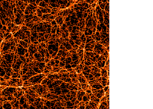
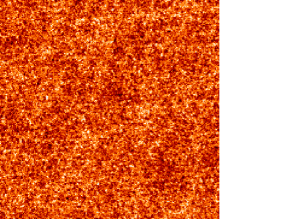
Figure 1.  : Numerical simulation of galaxy clustering (left) together with a version generated randomly reshuffling the phases between Fourier modes of the original picture (right).

Since the amplitude of each Fourier mode is unchanged in the phase reshuffling operation, these two pictures have exactly the same power-spectrum, $P(k)\propto|\tilde{\delta}({\bf k})|^{2}$. In fact, they have more than that: they have exactly the same amplitudes for all ${\bf k}$. They also have totally different morphology. Further demonstrations of the importance of Fourier phases in defining clustering morphology are given by Chiang (2001).

5.1 Quadratic density fields

It is useful at this stage to a particular form of non-Gaussian field that serves both as a kind of phenomenological paradigm and as a reasonably realistic model of non-linear evolution from Gaussian initial conditions. The model involves a field which is generated by a simple quadratic transformation of a Gaussian distribution, hence the term quadratic non-linearity. Quadratic fields have been discussed before from a number of contexts (e.g. Coles & Barrow 1987; Moscardini et al. 1991; Falk, Rangarajan & Srednicki 1993; Luo & Schramm 1993; Luo 1994; Gangui et al. 1994; Koyoma, Soda & Taruya 1999; Peebles 1999a,b; Matarrese, Verde & Jimenez 2000; Verde et al. 2000; Verde et al. 2001; Komatsu & Spergel 2001; Shandarin 2002; Bartolo, Matarrese & Riotto 2002); for further discussion see below. The motivation is very similar to that of Coles & Jones (1991), which introduced the lognormal density field as an illustration of some of the consequences of a more extreme form of non-linearity involving an exponential transformation of the linear density field.

5.2 A simple non-linear model

We adopt the simple perturbative expansion of equation (20) in order to model the non-linear evolution of the density field. Although the equivalent transformation in formal Eulerian perturbation theory is a good deal more complicated, the kind of phase associations that we will deal with here are precisely the same in either case. In terms of the Fourier modes, in the continuum limit, we have for the first order Gaussian term

$$\delta_{1}({\bf x})=\int d^{3}k\,\,|\delta_{\bf k}|\exp{[i\phi_{\bf k}]}\exp{[i{\bf k}\cdot{\bf x}]}$$ (33)

and for the second-order perturbation

$$\delta_{2}({\bf x})=\left[\delta_{1}({\bf x})\right]^{2}=\int d^{3}k\,d^{3}k^{\prime}\,\,|\delta_{\bf k}||\delta_{\bf k^{\prime}}|\exp{[i(\phi_{\bf k}+\phi_{\bf k^{\prime}})]}\,\exp{[i({\bf k}+{\bf k}^{\prime})\cdot{\bf r}]}.$$ (34)

The quadratic field, $\delta_{2}$, illustrates the idea of mode coupling associated with non-linear evolution. The non-linear field depends on a specific harmonic relationship between the wavenumber and phase of the modes at ${\bf k}$ and ${\bf k}^{\prime}$. This relationship between the phases in the non-linear field, i.e.

$$\phi_{{\bf k}}+\phi_{{\bf k}^{\prime}}=\phi_{{\bf k}+{\bf k}^{\prime}},$$ (35)

where the RHS represents the phase of the non-linear field, is termed quadratic phase coupling.

5.3 The two-point covariance function

The two-point covariance function can be calculated using the definitions of §2, namely

$$\xi(r)=\langle\delta({\bf x})\delta({\bf x}+{\bf r})\rangle.$$ (36)

Substituting the non-linear transform for $\delta({\bf x})$ (equation 20) into this expression gives four terms

$$\xi(r)=\langle\delta_{1}({\bf x})\delta_{1}({\bf x}+{\bf r})\rangle+\epsilon\langle\delta_{1}({\bf x})\delta_{2}({\bf x}+{\bf r})\rangle+\epsilon\langle\delta_{2}({\bf x})\delta_{1}({\bf x}+{\bf r})\rangle+\epsilon^{2}\langle\delta_{2}({\bf x})\delta_{2}({\bf x}+{\bf r})\rangle.$$ (37)

The first of these terms is the linear contribution to the covariance function whereas the remaining three give the non-linear corrections. We shall focus on the lowest order term for now.

As we outlined in Section 2, the angle brackets $\langle\rangle$ in these expressions are expectation values, formally denoting an average over the probability distribution of $\delta({\bf x})$. Under the fair sample hypothesis we replace the expectation values in equation (36) with averages over a selection of independent volumes so that $\langle\rangle\rightarrow\langle\rangle_{\mbox{\small{vol, real}}}$. The first average is simply a volume integral over a sufficiently large patch of the universe. The second average is over various realisations of the $\delta_{k}$ and $\phi_{k}$ in the different patches. Applying these rules to the first term of equation (37) and performing the volume integration gives

$$\xi_{11}(r)=\int d^{3}k\,d^{3}k^{\prime}\,\,\langle|\delta_{\bf k}||\delta_{\bf k^{\prime}}|\exp{[i(\phi_{\bf k}+\phi_{\bf k^{\prime}})]}\rangle_{\mbox{\small{real}}}\,\delta_{D}({\bf k}+{\bf k}^{\prime})\exp{[i{\bf k}^{\prime}\cdot{\bf s}]},$$ (38)

where $\delta_{D}$ is the Dirac delta function. The above expression is simplified given the reality condition

$$\delta_{{\bf k}}=\delta^{*}_{-{\bf k}},$$ (39)

from which it is evident that the phases obey

$$\phi_{{\bf k}}+\phi_{-{\bf k}}=0\,\,\,\mbox{mod}[2\pi].$$ (40)

Integrating equation (38) one therefore finds that

$$\xi_{11}(r)=\int d^{3}k\,\,\langle|\delta_{\bf k}|^{2}\rangle_{\mbox{\small{real}}}\exp{[-i{\bf k}\cdot{\bf s}]}.$$ (41)

so that the final result is independent of the phases. Indeed this is just the Fourier transform relation between the two-point covariance function and the power spectrum we derived in §2.1.

5.4 The three-point covariance function

Using the same arguments outlined above it is possible to calculate the 3-point connected covariance function, which is defined as

$$\zeta({\bf r},{\bf s})=\langle\delta({\bf x})\delta({\bf x}+{\bf r})\delta({\bf x}+{\bf s})\rangle_{c}.$$ (42)

Making the non-linear transform of equation (20) one finds the following contributions

$$\zeta({\bf r},{\bf s}) = \langle\delta_{1}({\bf x})\delta_{1}({\bf x}+{\bf r})\delta_{1}({\bf x}+{\bf s})\rangle_{c}+\epsilon\langle\delta_{1}({\bf x})\delta_{1}({\bf x}+{\bf r})\delta_{2}({\bf x}+{\bf s})\rangle_{c}$$ (43)

$$+\mbox{perms}(121,211)+\epsilon^{2}\langle\delta_{1}({\bf x})\delta_{2}({\bf x}+{\bf r})\delta_{2}({\bf x}+{\bf s})\rangle_{c}$$

$$+\mbox{perms}(212,221)+\epsilon^{3}\langle\delta_{2}({\bf x})\delta_{2}({\bf x}+{\bf r})\delta({\bf x}+{\bf s})\rangle_{c}.$$

Again we consider first the lowest order term. Expanding in terms of the Fourier modes and once again replacing averages as prescribed by the fair sample hypothesis gives

$$\zeta_{111}({\bf r},{\bf s}) = \int d^{3}k\,d^{3}k^{\prime}\,d^{3}k^{\prime\prime}\,\,\,\langle|\delta_{\bf k}||\delta_{\bf k^{\prime}}||\delta_{\bf k^{\prime\prime}}|\exp{[i(\phi_{\bf k}+\phi_{\bf k^{\prime}}+\phi_{\bf k^{\prime\prime}})]}\rangle_{\mbox{\small{real}}}$$ (44)

$$\times\delta_{D}({\bf k}+{\bf k}^{\prime}+{\bf k}^{\prime\prime})\exp{[i{\bf k}^{\prime}\cdot{\bf r}]}\exp{[i{\bf k}^{\prime\prime}\cdot{\bf s}]}.$$

Recall that $\delta_{1}$ is a Gaussian field so that $\phi_{\bf k}$, $\phi_{\bf k^{\prime}}$ and $\phi_{\bf k^{\prime\prime}}$ are independent and uniformly random on the interval $[0,2\pi]$. Upon integration over one of the wavevectors the phase terms is modified so that its argument contains the sum $(\phi_{\bf k}+\phi_{\bf k^{\prime}}+\phi_{-{\bf k}-{\bf k}^{\prime\prime}})$, or a permutation thereof. Whereas the reality condition of equation (39) implies a relationship between phases of anti-parallel wavevectors, no such conditions hold for modes linked by the triangular constraint imposed by the Dirac delta function. In other words, except for serendipity,

$$\phi_{\bf k}+\phi_{\bf k^{\prime}}+\phi_{-{\bf k}-{\bf k}^{\prime\prime}}\neq 0.$$ (45)

In fact due to the circularity of phases, the resulting sum is still just uniformly random on the interval $[0,2\pi]$ if the phases are random. Upon averaging over sufficient realisations, the phase term will therefore cancel to zero so that the lowest order contribution to the 3-point function vanishes, i.e. $\zeta_{111}({\bf r},{\bf s})=0$. This is not a new result, but it does explicitly illustrate how the vanishing of the three-point connected covariance function arises in terms of the Fourier phases.

Next consider the first non-linear contribution to the 3-point function given by

$$\zeta_{112}({\bf r},{\bf s})=\epsilon\langle\delta_{1}({\bf x})\delta_{1}({\bf x}+{\bf r})\delta_{2}({\bf x}+{\bf s})\rangle,$$ (46)

or one of its permutations. In this case one of the arguments in the average is the field $\delta_{2}({\bf x})$, which exhibits quadratic phase coupling of the form (35). Expanding this term to the point of equation (44) using the definition (34) one obtains

$$\zeta_{112}({\bf r},{\bf s}) = \int d^{3}k\,d^{3}k^{\prime}\,d^{3}k^{\prime\prime}\,d^{3}k^{\prime\prime\prime}\,\,\,$$ (47)

$$\langle|\delta_{\bf k}||\delta_{\bf k^{\prime}}||\delta_{\bf k^{\prime\prime}}||\delta_{\bf k^{\prime\prime\prime}}|\exp{[i(\phi_{\bf k}+\phi_{\bf k^{\prime}}+\phi_{\bf k^{\prime\prime}}+\phi_{\bf k^{\prime\prime\prime}})]}\rangle_{\mbox{\small{real}}}$$

$$\times\delta_{D}({\bf k}+{\bf k}^{\prime}+{\bf k}^{\prime\prime}+{\bf k}^{\prime\prime\prime})$$

$$\times\exp{[i{\bf k}^{\prime}\cdot{\bf r}]}\exp{[i({\bf k}^{\prime\prime}+{\bf k}^{\prime\prime\prime})\cdot{\bf s}]}.$$

Once again the Dirac delta function imposes a general constraint upon the configuration of wavevectors. Integrating over one of the ${\bf k}$ gives ${\bf k}^{\prime\prime\prime}=-{\bf k}-{\bf k}^{\prime}-{\bf k}^{\prime\prime}$ for example, so that the wavevectors must form a closed loop. This general constraint however, does not specify a precise shape of loop, instead the remaining integrals run over all of the different possibilities. At this point we may constrain the problem more tightly by noting that most combinations of the ${\bf k}$ will contribute zero to $\zeta_{(112)}$. This is because of the circularity property of the phases and equation (45). Indeed, the only nonzero contributions arise where we are able to apply the phase relation obtained from the reality constraint, equation (40). In other words the properties of the phases dictate that the wavevectors must align in anti-parallel pairs: ${\bf k}=-{\bf k}^{\prime}$, ${\bf k}^{\prime\prime}=-{\bf k}^{\prime\prime\prime}$ and so forth.

There is a final constraint that must be imposed upon the ${\bf k}$ if $\zeta$ is the connected $3$-point covariance function. In a graph theoretic sense, the general (unconnected) $N$-point function $\langle\delta_{l_{1}}({\bf x}_{1})\delta_{l_{2}}({\bf x}_{2})...\delta_{l_{N}}({\bf x}_{N})\rangle$ can be represented geometrically by a sum of tree diagrams. Each diagram consists of $N$ nodes of order $l_{i}$, representing the $\delta_{l_{i}}({\bf x}_{i})$, and a number of linking lines denoting their correlations; see Fry (1984) or Bernardeau (1992) for more detailed accounts. Every node is made up of $l_{i}$ internal points, which represent a factor $\delta_{{\bf k}}=|\delta_{\bf k}|\exp{(i\phi_{\bf k})}$ in the Fourier expansion. According to the rules for constructing diagrams, linking lines may join one internal point to a single other, either within the same node or in an external node. The connected covariance functions are represented specifically by the subset of diagrams for which every node is linked to at least one other, leaving none completely isolated. This constraint implies that certain pairings of wavevectors do not contribute to the connected covariance function. For more details, see Watts & Coles (2002).

The above constraints may be inserted into equation (47) by re-writing the Dirac delta function as a product over Delta functions of two arguments, appropriately normalised. There are only two allowed combinations of wavevectors so we have

$$\delta_{D}({\bf k}+{\bf k}^{\prime}+{\bf k}^{\prime\prime}+{\bf k}^{\prime\prime\prime})\rightarrow\frac{1}{2V_{u}}[\delta_{D}({\bf k}+{\bf k}^{\prime\prime})\delta_{D}({\bf k}^{\prime\prime\prime}+{\bf k}^{\prime\prime\prime})+\delta_{D}({\bf k}+{\bf k}^{\prime\prime\prime})\delta_{D}({\bf k}^{\prime}+{\bf k}^{\prime\prime})].$$ (48)

Integrating over two of the ${\bf k}$ and using equation (40) eliminates the phase terms and leaves the final result

$$\zeta_{112}({\bf r},{\bf s})=\frac{1}{V_{u}}\int d^{3}k\,d^{3}k^{\prime}\,\,\langle|\delta_{\bf k}|^{2}|\delta_{\bf k^{\prime}}|^{2}\rangle_{\mbox{\small{real}}}\exp{[i{\bf k}^{\prime}\cdot{\bf r}]}\exp{[-i({\bf k}+{\bf k}^{\prime})\cdot{\bf s}]}.$$ (49)

The existence of this quantity has therefore been shown to depend on the quadratic phase coupling of Fourier modes. The relationship between modes and the interpretation of the tree diagrams is also dictated by the properties of the phases.

One may apply the same rules to the higher order terms in equation (43). It is immediately clear that the $\zeta_{122}$ terms are zero because there is no way to eliminate the phase term $\exp{[i(\phi_{\bf k}+\phi_{\bf k^{\prime}}+\phi_{\bf k^{\prime\prime}}+\phi_{\bf k^{\prime\prime\prime}}+\phi_{{\bf k}^{\prime\prime\prime\prime}})]}$, a consequence of the property equation (45). Diagrammatically this corresponds to an unpaired internal point within one of the nodes of the tree. The final, highest order contribution to the 3-point function is found to be

$$\zeta_{222}({\bf r},{\bf s}) = \frac{1}{V_{u}^{2}}\int d^{3}k\,d^{3}k^{\prime}\,d^{3}k^{\prime\prime}\,\,\langle|\delta_{\bf k}|^{2}|\delta_{\bf k^{\prime}}|^{2}|\delta_{\bf k^{\prime\prime}}|^{2}\rangle_{\mbox{\small{real}}}$$ (50)

$$\times\exp{[i({\bf k}-{\bf k}^{\prime})\cdot{\bf r}]}\exp{[i({\bf k}^{\prime}-{\bf k}^{\prime\prime})\cdot{\bf s}]},$$

where the phase and geometric constraints allow 12 possible combinations of wavevectors.

5.5 Cubic non-linearity and higher order

The above ideas extend simply to higher order where the non-linear field is represented by a perturbation series that does not truncate at the quadratic term. At the next highest order for example, the series includes $\delta_{3}=\delta_{1}^{3}$, which introduces a cubic phase coupling in the Fourier expansion. Although quadratic phase coupling is essential as a minimum requirement for the three point covariance function, cubic phase coupling is not the minimum requirement for the next highest order covariance function. Indeed, quadratic coupling is sufficient to provide contributions to all of the n-point covariance functions due to the way the phases dictate that wave-vectors must arrange themselves into antiparallel pairs. For the 4-point covariance function the cubic term allows for a different diagrammatic representation: a star as opposed to a snake topology. However, in terms of the constituent wave-vectors, loops (as in Figure 3) contributing to the star topologies are a symmetric subset of those contributing to the snake topologies.

5.6 Power-spectrum and Bispectrum

The formal development of the relationship between covariance functions and power-spectra developed above suggests the usefulness of higher–order versions of $P(k)$. It is clear from the arguments of Section 5.2 that a more convenient notation for the power-spectrum than that introduced in Section 2.1 is

$$\langle\delta_{{\bf k}}\delta_{{\bf k}^{\prime}}\rangle=(2\pi)^{3}P(k)\delta_{D}({\bf k}+{\bf k}^{\prime}).$$ (51)

The connection between phases and higher-order covariance functions obtained in Section 5.3 also suggests defining higher-order polyspectra of the form

$$\langle\delta_{{\bf k}}\delta_{{\bf k}^{\prime}}\ldots\delta_{{\bf k}^{(n)}}\rangle=(2\pi)^{3}P_{n}({\bf k},{\bf k}^{\prime},\ldots{\bf k}^{(n)})\delta_{D}({\bf k}+{\bf k}^{\prime}+\ldots{\bf k}^{(n)})$$ (52)

where the occurrence of the delta-function in this expression arises from a generalisation of the reality constraint given in equation (40); see, e.g., Peebles (1980). Conventionally the version of this with $n=3$ produces the bispectrum, usually called $B({\bf k},{\bf k}^{\prime},{\bf k}^{\prime\prime})$ which has found much effective use in recent studies of large-scale structure (Peebles 1980; Scoccimarro et al. 1998; Scoccimarro, Couchman & Frieman 1999; Verde et al. 2000; Verde et al. 2001; Verde et al. 2002). It is straightforward to show that the bispectrum is the Fourier-transform of the (reduced) three–point covariance function by following similar arguments as in Section 5.2; see, e.g., Peebles (1980).

Note that the delta-function constraint requires the bispectrum to be zero except for $k$-vectors (${\bf k}$, ${\bf k}^{\prime}$, ${\bf k}^{\prime\prime}$) that form a triangle in $k$-space. From Section 5.3 it is clear that the bispectrum can only be non-zero when there is a definite relationship between the phases accompanying the modes whose wave-vectors form a triangle. Moreover the pattern of phase association necessary to produce a real and non-zero bispectrum is precisely that which is generated by quadratic phase association. This shows, in terms of phases, why it is that the leading order contributions to the bispectrum emerge from second-order fluctuations of a Gaussian random field. The bispectrum measures quadratic phase coupling.

Three-point phase correlations have another interesting property. While the bispectrum is usually taken to be an ensemble-averaged quantity, as defined in equation (46), it is interesting to consider products of terms $\delta_{{\bf k}}\delta_{{\bf k}^{\prime}}\delta_{{\bf k}^{\prime\prime}}$ obtained from an individual realisation. According to the fair sample hypothesis discussed above we would hope appropriate averages of such quantities would yield an estimate of the bispectrum. Note that

$$\delta_{{\bf k}}\delta_{{\bf k}^{\prime}}\delta_{{\bf k}^{\prime\prime}}=\delta_{{\bf k}}\delta_{{\bf k}^{\prime}}\delta_{-{\bf k}-{\bf k}^{\prime}}=\delta_{{\bf k}}\delta_{{\bf k}^{\prime}}\delta^{*}_{{\bf k}+{\bf k}^{\prime}}\equiv\beta({\bf k},{\bf k}^{\prime}),$$ (53)

using the requirement (40), together with the triangular constraint we discussed above. Each $\beta({\bf k},{\bf k}^{\prime})$ will carry its own phase, say $\phi_{{\bf k},{\bf k}^{\prime}}$, which obeys

$$\phi_{{\bf k},{\bf k}^{\prime}}=\phi_{{\bf k}}+\phi_{{\bf k}^{\prime}}-\phi_{{\bf k}+{\bf k}^{\prime}}.$$ (54)

It is evident from this that it is possible to recover the complete set of phases $\phi_{{\bf k}}$ from the bispectral phases $\phi_{{\bf k},{\bf k}^{\prime}}$, up to a constant phase offset corresponding to a global translation of the entire structure (Chiang & Coles 2000). This furnishes a conceptually simple method of recovering missing or contaminated phase information in a consistent way, an idea which has been exploited, for example, in speckle interferometry (Lohmann, Weigelt & Wirnitzer 1983). In the case of quadratic phase coupling, described by equation (35), the left-hand-side of equation (54) is identically zero leading to a particularly simple approach to this problem.

6 Discussion

In this lecture I addressed two main issues, using the quadratic model as an illustrative example. First I showed explicitly how this non-Gaussian model has properties that contradict standard folklore based on the assumption of Gaussian fluctuations. We used this model to distinguish carefully between various inter-related concepts such as sample homogeneity, statistical homogeneity, asymptotic independence, ergodicity, and so on. I showed the conditions under which each of these is relevant and deployed the quadratic model for particular examples in which they are violated. I then used the quadratic model to show how phase association arises in non-linear processes which has exactly the correct form to generate non-zero bispectra and three–point covariance functions. The magnitude of these statistical descriptors is of course related to the magnitude of the Fourier modes, but the factor that determines whether they are zero or non-zero is the arrangement of the phases of these modes.

The connection between polyspectra and phase information is an important one and it opens up many lines of future research, such as how phase correlations relate to redshift distortion and bias. Also, I assumed throughout this study that we could straightforwardly take averages over a large spatial domain to be equal to ensemble averages. Using small volumes of course leads to sampling uncertainties which are quite straightforward to deal with in the case of the power-spectra but more problematic for higher-order spectra like the bispectrum. Understanding the fluctuations about ensemble averages in terms of phases could also lead to important insights.

References

- [] Adler R.J., 1981, The Geometry of Random Fields. John Wiley & Sons, New York.
- [] Bardeen J.M., Bond J.R., Kaiser N., Szalay A.S., 1986, ApJ, 304,
- [] Bartolo N., Matarrese S., Riotto A., 2002, Phys. Rev. D., 65, 103505
- [] Bernardeau F., 1992, ApJ, 392, 1
- [] Bernardeau F., Colombi S., Gaztanaga E., Scoccimarro R., 2002, Phys. Rep., in press, astro-ph/0112551
- [] Chiang L.-Y., 2001, MNRAS, 325, 405
- [] Chiang L.-Y., Coles P., 2000, MNRAS, 311, 809
- [] Chiang L.-Y., Coles P., Naselsky P., 2002, MNRAS, in press, astro-ph/0207584
- [] Coleman P.H., Pietronero L., 1992, Phys. Rep. 231, 311
- [] Coles P., 1993, MNRAS, 262, 1065
- [] Coles P., Barrow J.D., 1987, MNRAS, 228, 407
- [] Coles P., Chiang L.-Y., 2000, Nature, 406, 376
- [] Coles P., Jones B.J.T., 1991, MNRAS, 248, 1
- [] Coles P., Lucchin F., 2002, Cosmology: The Origin and Evolution of Cosmic Structure, 2nd Edition. John Wiley & Sons, Chichester
- [] Falk T., Rangarajan R., Srednicki M., 1993, ApJ, 403, L1
- [] Fan Z., Bardeen J.M., 1995, Phys. Rev. D., 51, 6714
- [] Fry J.N., 1984, ApJ, 279, 499
- [] Fry J.N., Gaztanaga E., 1993, ApJ, 413, 447
- [] Gangui A., Lucchin F., Matarrese S., Mollerach S., 1994, ApJ, 430, 447
- [] Guth A.H., 1981, Phys. Rev. D., 23, 347
- [] Guth A.H., Pi S.-Y., 1982, Phys. Rev. Lett., 49, 1110
- [] Hobson M.P., Jones A.W., Lasenby A., 1999, MNRAS, 309, 125
- [] Jain B., Bertschinger E., 1998, ApJ, 509, 517
- [] Kendall M., Stuart A., 1977, The Advanced Theory of Statistics, Vol. 1. Griffin & Co, London
- [] Komatsu E., Spergel D.N., 2001, Phys. Rev. D., 63, 063002
- [] Koyama K., Soda J., Taruya A., 1999, MNRAS, 310, 1111
- [] Lohmann A.W., Weigelt G., Wirnitzer B., 1983, Appl. Optics, 22, 4028
- [] Luo X., 1994, ApJ, 427, L71
- [] Luo X., Schramm D.N., 1993, ApJ, 408, 33
- [] Matarrese S., Verde L., Jimenez R., 2000, ApJ, 541, 10
- [] Moscardini L., Matarrese S., Lucchin F., Messina A., 1991, MNRAS, 248, 424
- [] Peacock J.A., Dodds S., 1996, MNRAS, 267, 1020
- [] Peebles P.J.E., 1980, The Large-Scale Structure of the Universe. Princeton University Press, Princeton NJ.
- [] Peebles P.J.E., 1999a, ApJ, 510, 523
- [] Peebles P.J.E., 1999b, ApJ, 510, 531
- [] Percival W.J. et al. 2001, MNRAS, 327, 1297
- [] Ryden B.S., Gramann M., 1991, ApJ, 383, L33
- [] Salopek D.S., 1992, Phys. Rev. D., 45, 1139
- [] Salopek D.S., Bond J.R., Phys. Rev. D., 42, 3936
- [] Scherrer R.J., Melott A.L., Shandarin S.F., 1991, ApJ, 377, 29
- [] Schmalzing J., Gorski K.M., 1998, MNRAS, 297, 355
- [] Scoccimarro R., Colombi S., Fry J.N., Frieman J.A., Hivon E., Melott A.L., 1998, ApJ, 496, 586
- [] Scoccimarro R., Couchman H.M.P., Frieman J.A., 1999, ApJ, 517, 531
- [] Shandarin S.F., 2002, MNRAS, 331, 865
- [] Soda J., Suto Y., 1992, ApJ, 396, 379
- [] Stirling A.J., Peacock J.A., 1996, MNRAS, 283, L99
- [] Verde L., Heavens A.F., 2001, ApJ, 553, 14
- [] Verde L., Jimenez R., Kamionkowski M., Matarrese S., 2001, MNRAS, 325, 412
- [] Verde L., Wang L., Heavens A.F., Kamionkowski M., 2000, MNRAS, 313, 141
- [] Verde L. et al. 2002, MNRAS, 335, 432
- [] Wang L., Kamionkowski M., 2000, Phys. Rev. D., 61, 063504
- [] Watts P.I.R., Coles P., 2002, MNRAS, in press, astro-ph/0208295