Molecular abundances in carbon-rich circumstellar envelopes

A millimetre molecular line survey of seven high mass-loss rate carbon stars in both the northern and southern skies is presented. A total of 196 emission lines (47 transitions) from 24 molecular species were detected. The observed CO emission is used to determine mass-loss rates and the physical structure of the circumstellar envelope, such as the density and temperature structure, using a detailed radiative transfer analysis. This enables abundances for the remaining molecular species to be determined. The derived abundances generally vary between the sources by no more than a factor of five indicating that circumstellar envelopes around carbon stars with high mass-loss rates have similar chemical compositions. However, there are some notable exceptions. The most striking difference between the abundances are reflecting the spread in the ¹²C/¹³C-ratio of about an order of magnitude between the sample stars, which mainly shows the results of nucleosynthesis. The abundance of SiO also shows a variation of more than an order of magnitude between the sources and is on the average more than an order of magnitude more abundant than predicted from photospheric chemistry in thermal equilibrium. The over-abundance of SiO is consistent with dynamical modelling of the stellar atmosphere and the inner parts of the wind where a pulsation-driven shock has passed. This scenario is possibly further substantiated by the relatively low amount of CS present in the envelopes. The chemistry occurring in the outer envelope is consistent with current photochemical models.

1 Introduction

The chemistry associated with carbon stars has long been known to be rich and complex in comparison to the alternative O-rich regime (i.e., where C/O $<$ 1). This is in part due to the favourable bonding of the carbon atom, enabling long chains and complex species to form. Most of the current understanding of carbon stars has come from both observational and theoretical work on the high-mass-losing carbon star, IRC+10216. This source, which lies within 200 pc and presents an ideal specimen for the study of carbon-rich envelopes, has been mapped interferometrically in various molecular species (e.g. Bieging & Tafalla 1993; Dayal & Bieging 1993, 1995; Gensheimer et al. 1995; Guelin et al. 1993, 1996; Lucas et al. 1995; Lucas & Guélin 1999) and has had models of its dust (a good summary is given by Men’shchikov et al. 2001) and chemistry (e.g. Millar et al. 2000) constructed. These tools have produced groundbreaking results and have been used to set a paradigm for what has come to be known as “carbon chemistry” in connection with evolved stars. However, the accuracy of employing IRC+10216 chemistry to similar carbon stars has been little-tested due to the difficulties in observing them. Much work has been done on the carbon-rich post-AGB sources CRL 618 and CRL 2688, and the chemistry of CRL 618 in particular has been modelled by Woods et al. (2002). Detailed chemical studies of carbon stars on the AGB have been few in number, but examples include the molecular line survey of IRAS 15194–5115, a peculiar ¹³C-rich star (Nyman et al. 1993). Carbon star surveys which include molecular-line comparisons are fewer, and have been limited in the number of lines observed. Olofsson et al. (1993a) detected some 40 stars in a handful of species other than CO. The sample of Bujarrabal et al. (1994) included 16 carbon stars, with up to ten molecular lines observed in each. A more recent survey by Olofsson et al. (1998) detected 22 carbon stars in up to 6 molecular lines.

Table 1: Positions, luminosities, periods and calculated distances of the sample of carbon stars.

IRAS No.	Other cat. name	B1950 Co-ords.	$P$	$L$	$D$	$T_{*}$	$T_{\mathrm{d}}$	$L_{\mathrm{d}}$/$L_{*}$
			[days]	[L⊙]	[pc]	[K]	[K]
$07454-7112$	AFGL 4078	07:45:25.7 $-$71:12:18	—	9 000a	710	1 200	0710	4.3
$09452+1330$	IRC+10216	09:45:15.0 $+$13:30:45	630	9 600b	120	—	0510	—
$10131+3049$	CIT 6	10:13:11.5 $+$30:49:17	640	9 700b	440	1 300	0510	6.7
$15082-4808$	AFGL 4211	15:08:13.0 $-$48:08:43	—	9 000a	640	—	0590	—
$15194-5115$	—	15:19:26.9 $-$51:15:19	580	8 800b	600	0930	0480	2.2
$23166+1655$	AFGL 3068	23.16.42.4 $+$16:55:10	700	7 800b	820	—	1 000	—
$23320+4316$	IRC+40540	23:32:00.4 $+$43:16:17	620	9 400b	630	1 100	0610	6.6

1. Assumed value.

The survey work presented here purports to be the most complete and consistent molecular-line survey in AGB carbon stars to date, covering high mass-loss rate objects in both the northern and the southern sky. Previously unpublished spectra of five stars (IRAS 15082–4808, IRAS 07454–7112, CIT 6, AFGL 3068 and IRC+40540) are presented, and spectra taken towards IRC+10216 and IRAS 15194–5115 with the Swedish-ESO Submillimetre Telescope (SEST; Nyman et al. 1993) and IRC+10216 with the Onsala Space Observatory (OSO) 20 m telescope are used to supplement the survey. Comparison of data from IRC+10216 taken with both telescopes affords a high degree of confidence in the relative calibration that can be derived.

Up to 51 molecular lines were observed in the sample of 7 high-mass-losing carbon stars, of which 47 were clearly detected. Mass-loss rates, dust properties and the ¹²CO/¹³CO-ratio are calculated self-consistently using a radiative transfer method (Schöier & Olofsson 2000, 2001; Schöier et al. 2002). An approach similar to that of Nyman et al. (1993) is adopted to calculate fractional abundances (including upper limits), and a detailed analysis of the comparison between the calculated abundances is carried out. Hence, Sect. 2 details the observations carried out and the instrumentation used. Section 3 gives the observational results, including a presentation of various spectra. Section 4 details the NLTE radiative transfer code used to determine the envelope parameters and Sect. 5 explains the method of calculating chemical abundances. The results and deductions are discussed in Sect. 6.

2 Observations

2.1 Carbon star sample

Following the CO survey of Nyman et al. (1992), several carbon stars, which were bright in CO lines, were selected for a more comprehensive molecular line search. These stars are rare in that they are all losing mass at a very high rate, and hence are more likely to produce strong emission from a variety of molecular lines. The sample of seven carbon stars (Table 1) was observed using both the 15 m Swedish–ESO Submillimetre Telescope (Booth et al. 1989) during the period 1987 – 1996, and the Onsala 20 m telescope, in 1994. The SEST, situated on La Silla, Chile, was used to observe IRAS 07454-7112, IRAS 15082-4808, and IRAS 15194-5115. The 20 m telescope, located at the Onsala Space Observatory (OSO) in Sweden, observed the remaining three sources, CIT 6, AFGL 3068 and IRC +40540. Both telescopes were used to observe the well-studied carbon star, IRC +10216 in order to determine the relative calibration between the two telescopes.

The JCMT public archive was searched for complementary line observations, in particular the CO lines used in the radiation transfer modelling described in Sect. 4. Lines for which multi-epoch observations are available in the JCMT archive typically display intensities that are consistent to $\sim$20% (Schöier & Olofsson 2001). In addition, interferometric observations of the CO($J$=1–0) brightness distribution around some of the sample stars have been performed (Neri et al. 1998) using the Plateu de Bure interferometer (PdBI), France. The data are publically available and have been used in this paper.

The coordinates used for each individual source are listed in Table 1. Also shown in Table 1 are the adopted luminosities and distances to be used in the molecular excitation analysis. For stars where a period has been determined (see Table 1) the period-luminosity relation from Groenewegen & Whitelock (1996) was used to estimate the corresponding luminosity. If a reliable period is not available the total bolometric luminosity was fixed to 9 000 L_☉. The distance was then obtained from the luminosity using the observed bolometric magnitude. Schöier & Olofsson (2001) used the same approach when determining the distances to a large sample of optically bright carbon stars and concluded that there were no apparent systematic effect when comparing with estimates based upon Hipparcos parallaxes, although the scatter is large and the distance estimate for an individual source is subject to some uncertainty of up to a factor of $\sim$2. The effects of the adopted distance on the molecular excitation will be addressed in Sect. 5.5.

If, for simplicity, the central ratiation field is represented by one or two blackbodies their properties can be determined from a fit to the observed spectral energy distribution (SED) as described in Kerschbaum (1999). A fit to the SED gives the two blackbody temperatures ($T_{*}$ and $T_{\mathrm{d}}$) as well as their relative luminosities ($L_{\mathrm{d}}$/$L_{*}$). The parameters obtained in this fashion are presented in Table 1.

2.2 Instrumentation

Table 2: Beam widths and efficiencies at selected frequencies.

	SEST 15 m			Onsala 20 m
Frequency	FWHM	$\eta_{\rm mb}$		FWHM	$\eta_{\rm mb}$
[GHz]	[$\arcsec$]			[$\arcsec$]
086	57	0.75		44	0.58
100	51	0.73		39	0.53
115	45	0.70		33	0.48
230	23	0.50		—	—
265	21	0.42		—	—

The SEST is equipped with two acousto-optical spectrometers (HRS, 86 MHz bandwidth with 43 kHz channel separation and 80 kHz resolution; LRS, 500 MHz bandwidth with 0.7 MHz channel separation and a resolution of 1.4 MHz). The receivers used were dual polarization Schottky receivers at both 3 and 1.3 mm wavelength. Typical system temperatures above the atmosphere were 400–500 K and 1000-1800 K, respectively.

The OSO 20 m telescope uses two filterbanks (MUL B, 64 MHz bandwidth with a channel width of 250 kHz; MUL A, 512 MHz bandwidth and a channel width of 1 MHz). The receiver used was a horizontally, linearly polarised SIS receiver with a typical system temperature of 400–500 K above the atmosphere.

All observations were performed using the dual beam switching method, which places the source alternately in two beams, and yields very flat baselines. Beam separation was in both cases about 11$\aas@@fstack{\prime}$5. Calibration was done with the standard chopper-wheel method. The intensity scales of the spectra are given in main-beam brightness temperature (the corrected antenna temperature, $T_{\mathrm{A}}^{*}$, divided by the main-beam efficiency, $\eta_{\mathrm{mb}}$). Main-beam efficiencies and FWHM beam widths are given in Table 2 for both telescopes.

3 Observational results

Figure 1: Low-resolution spectra of IRAS07454–7112, obtained with the SEST.

Figure 2: Low-resolution spectra of IRAS07454–7112, obtained with the SEST.

3.1 Observed lines

A total of 196 lines were detected in the sample. 47 transitions of 24 molecular species were detected, and upper limits for another 95 relevant transitions were also obtained, including another three species (C₂S, C₃S and SO). Previously unpublished spectra are shown in Figs. 1–2 & 5–17. Table 3 lists the detections in all seven sources, together with their peak and integrated intensities. If a line has a hyperfine structure, the frequency and intensity of the strongest component is listed, and the integrated intensity is the sum over all hyperfine components. Values of $T_{\mathrm{mb}}$ for lines where no detection was made are the rms noise values.

Almost all lines observed in IRC+10216 by the SEST were observed in the same source with the OSO 20 m telescope. The majority of those which were not are due to the lack of a 1.3 mm receiver at OSO. A large proportion of these lines were observed in the remaining six sources. The purpose of observing IRC+10216 twice, with different telescopes, was to ascertain the relative calibration between the two different setups, and hence gain a basis from which good comparisons could be made between the entire sample of carbon stars.

The ¹³CS ($J$=2–1) line observed in some of these sources is partially blended with the C₃S ($J$=16–15) line (Kahane et al. 1988). The ¹³CS ($J$=2–1) integrated intensities include both these lines. It is assumed that the relative intensities of these two lines are constant in all the objects, and hence will not affect comparisons. The lines of two HC₃N isotopes, HC¹³CCN and HCC¹³CN, lie very closely and are in all cases blended together. No attempt is made to separate the components.

3.2 Line profiles

There are four characteristic line profile shapes which give information on the source being observed. These lineshapes are most typically seen in CO emission since it is often strongest (for a comprehensive review of line profiles see Olofsson et al. 1993b). For optically thick emission the line profile can be described as parabolic for unresolved sources or flat-topped for resolved sources. A parabolic profile is shown by most of the ¹²CO emission lines in the sample except in IRC+10216 and IRAS 15194–5115, where the CO ($J$=1–0) emission shows a flat-topped profile.

When emission is optically thin, a flat-topped profile is seen for unresolved sources, and a double-peaked profile for a resolved source. Examples of these profiles can be seen in the ¹³CO emission towards IRAS 15082–4808 and IRC+10216. In the following calculations, all lines are assumed optically thin, except those from CO and HCN.

The values of the expansion velocity, $v_{\mathrm{exp}}$, of the circumstellar envelopes quoted in Table 4 are obtained from the radiative transfer CO modelling of these sources (presented in Sect. 4) where its value is adjusted until a good fit to the observed line profiles is obtained. No trends in the widths of the observed lines are present which lends further support to the assumption adopted here that these envelopes are expanding at constant velocities.

Table 3: Detected lines

Molecule	Transition	Frequency		IRC+10216 (SEST)			IRC+10216 (OSO)			IRAS15194-5115			IRAS15082-4808
				$T_{\rm mb}$	$\int T_{\rm mb}{\rm d}v$		$T_{\rm mb}$	$\int T_{\rm mb}{\rm d}v$		$T_{\rm mb}$	$\int T_{\rm mb}{\rm d}v$		$T_{\rm mb}$	$\int T_{\rm mb}{\rm d}v$
		[MHz]		[K]	[K kms-1]		[K]	[K kms-1]		[K]	[K kms-1]		[K]	[K kms-1]
HC5N	J=32–31	085201.348		0.15	4.78		—	—		$<$ 0.01	$<$ 0.13		$<$ 0.01	$<$ 0.10
C3H2	21,2–10,1	085338.905		0.11	2.49		—	—		0.02	0.84		$<$ 0.01	$<$ 0.10
C4H	N=9–8, J=19/2–17/2	085634.00		0.20	9.60		—	—		—	—		$<$ 0.01	$<$ 0.05
C4H	N=9–8, J=17/2–15/2	085672.57		0.20	9.60		—	—		—	—		$<$ 0.01	$<$ 0.05
C2S	6(7)–5(6)	086181.413		$<$ 0.03	$<$ 0.46		$<$ 0.04	$<$ 0.76		$<$ 0.07	$<$ 0.11		$<$ 0.04	$<$ 0.06
H13CN	J=1–0	086340.184		3.23	87.20		3.86	114.14		0.57	20.93		0.09	3.06
C3S	J=15–14	086708.379		$<$ 0.02	$<$ 0.30		$<$ 0.03	$<$ 0.65		$<$ 0.01	$<$ 0.08		$<$ 0.01	$<$ 0.06
SiO	J=2–1	086846.998		0.71	20.40		0.95	24.48		0.16	5.33		0.07	1.84
HN13C	J=1–0	087090.859		$<$ 0.04	$<$ 0.62		—	—		0.02	1.11		$<$ 0.01	$<$ 0.11
C2H	N=1–0	087316.925		0.52	41.60		0.66	49.48		0.13	11.50		0.04	4.04
HCN	J=1–0	088631.847		7.80	190.93		9.14	214.04		0.55	15.33		0.37	11.26
C3N	N=9–8, J=19/2–17/2	089045.59		0.31	9.19		—	—		$<$ 0.01	$<$ 0.07		$<$ 0.01	$<$ 0.09
C3N	N=9–8, J=17/2–15/2	089064.36		0.31	9.19		—	—		$<$ 0.01	$<$ 0.07		$<$ 0.01	$<$ 0.09
HC5N	J=34–33	090525.892		0.16	2.58		$<$ 0.03	$<$ 0.67		—	—		$<$ 0.01	$<$ 0.10
HC13CCN	J=10–9	090593.059		0.09	1.98		$<$ 0.03	$<$ 0.34		0.02	0.76		$<$ 0.01	$<$ 0.05
HCC13CN	J=10–9	090601.791		0.09	1.98		$<$ 0.03	$<$ 0.34		0.02	0.76		$<$ 0.01	$<$ 0.05
HNC	J=1–0	090663.543		0.74	26.49		0.58	17.22		0.08	3.72		0.05	1.70
SiS	J=5–4	090771.546		1.14	35.54		1.07	39.47		0.05	2.78		0.03	1.58
HC3N	J=10–9	090978.993		2.42	64.59		2.00	52.63		0.09	3.71		0.11	4.15
13CS	J=2–1	092494.299		0.07	2.97		—	—		0.06	2.67		$<$ 0.01	$<$ 0.10
SiC2	40,4–30,3	093063.639		0.46	14.60		—	—		—	—		0.03	0.40
HC5N	J=35–34	093188.127		0.12	5.50		—	—		—	—		$<$ 0.01	$<$ 0.10
C4H	N=10–9, J=21/2–19/2	095150.32		0.19	6.08		0.18	8.75		0.04	1.95		0.02	0.47
C4H	N=10–9, J=19/2–17/2	095188.94		0.19	6.08		0.18	8.75		0.04	1.95		0.02	0.47
SiC2	42,2–32,1	095579.389		0.32	10.73		—	—		—	—		$<$ 0.01	$<$ 0.08
C34S	J=2–1	096412.982		0.15	5.66		—	—		—	—		—	—
CS	J=2–1	097980.968		2.92	81.23		4.06	118.89		0.37	15.21		0.25	8.44
C3H	${}^{2}\Pi_{1/2}$,9/2–7/2	097995.450		0.18	11.27		0.28	14.54		0.01	0.64		$<$ 0.01	$<$ 0.11
SO	J=3–2	099299.879		$<$ 0.02	$<$ 0.25		—	—		—	—		—	—
HC3N	J=11–10	100076.389		2.21	53.84		—	—		—	—		—	—
HC13CCN	J=12–11	108710.523		0.09	2.34		0.14	1.22		0.01	0.39		$<$ 0.01	$<$ 0.03
HCC13CN	J=12–11	108721.008		0.09	2.34		0.14	1.22		0.01	0.39		$<$ 0.01	$<$ 0.03
13CN	N=1–0	108780.201		0.11	8.56		0.24	6.07		0.02	2.18		$<$ 0.01	$<$ 0.05
C3N	N=11–10, J=23/2–21/2	108834.27		0.39	11.76		0.64	18.00		0.01	0.68		0.02	0.63
C3N	N=11–10, J=21/2–19/2	108853.02		0.39	11.76		0.64	18.00		0.01	0.68		0.02	0.63
SiS	J=6–5	108924.267		1.10	30.00		1.86	52.40		0.05	2.44		0.04	1.14
HC3N	J=12–11	109173.634		2.03	52.39		—	—		0.07	3.16		0.08	2.79
C18O	J=1–0	109782.160		0.02	0.76		—	—		—	—		$<$ 0.01	$<$ 0.17
13CO	J=1–0	110201.353		1.69	26.62		2.50	36.40		0.31	14.93		0.06	1.82
CH3CN	6(1)–5(1)	110381.404		0.09	4.77		$<$ 0.05	$<$ 1.42		$<$ 0.01	$<$ 0.18		$<$ 0.01	$<$ 0.23
C2S	8(9)–7(8)	113410.207		$<$ 0.03	$<$ 0.48		$<$ 0.07	$<$ 1.96		$<$ 0.02	$<$ 0.53		$<$ 0.01	$<$ 0.11
CN	N=1–0	113490.982		3.43	238.43		3.88	310.20		0.13	16.43		0.19	14.71
CO	J=1–0	115271.204		10.29	269.43		20.83	542.71		1.27	55.86		1.11	36.71
SiC2	50,5–40,4	115382.38		0.80	21.43		1.60	39.38		0.07	2.66		0.03	0.82
C18O	J=2–1	219560.319		0.15	4.21		—	—		—	—		—	—
13CO	J=2–1	220398.686		3.85	79.62		—	—		0.90	35.58		0.15	5.76
CH3CN	12(0)–11(0)	220747.268		0.17	2.80		—	—		$<$ 0.05	$<$ 1.01		$<$ 0.03	$<$ 0.48
CN	N=2–1	226874.564		2.55	231.18		—	—		0.15	17.06		0.20	11.32
CO	J=2–1	230538.000		34.60	799.00		—	—		4.20	150.00		2.54	69.40
CS	J=5–4	244935.606		16.57	405.53		—	—		0.77	32.34		0.47	10.89
HCN	J=3–2	265886.432		45.10	1010.24		—	—		4.69	139.76		0.88	20.83

Table 3: (cont.) Detected lines

Molecule	Transition	Frequency		IRAS07454-7112			CIT 6			AFGL 3068			IRC+40540
				$T_{\rm mb}$	$\int T_{\rm mb}{\rm d}v$		$T_{\rm mb}$	$\int T_{\rm mb}{\rm d}v$		$T_{\rm mb}$	$\int T_{\rm mb}{\rm d}v$		$T_{\rm mb}$	$\int T_{\rm mb}{\rm d}v$
		(MHz)		(K)	(K kms-1)		(K)	(K kms-1)		(K)	(K kms-1)		(K)	(K kms-1)
C2S	6(7)–5(6)	086181.413		$<$ 0.01	$<$ 0.07		$<$ 0.02	$<$ 0.36		$<$ 0.02	$<$ 0.44		$<$ 0.01	$<$ 0.28
H13CN	J=1–0	086340.184		0.07	1.45		0.15	3.13		0.13	3.76		0.13	3.85
C3S	J=15–14	086708.379		$<$ 0.01	$<$ 0.07		$<$ 0.01	$<$ 0.23		$<$ 0.02	$<$ 0.47		$<$ 0.01	$<$ 0.21
SiO	J=2–1	086846.998		0.03	0.52		0.17	3.16		$<$ 0.02	$<$ 0.47		0.04	0.94
HN13C	J=1–0	087090.859		$<$ 0.01	$<$ 0.08		$<$ 0.01	$<$ 0.23		$<$ 0.02	$<$ 0.47		$<$ 0.01	$<$ 0.25
C2H	N=1–0	087316.925		$<$ 0.01	$<$ 0.09		0.10	5.81		0.09	5.94		$<$ 0.01	$<$ 1.78
HCN	J=1–0	088631.847		0.19	4.43		0.77	18.07		0.39	8.97		0.26	8.24
C3N	N=9–8, J=19/2–17/2	089045.59		$<$ 0.01	$<$ 0.07		—	—		—	—		—	—
C3N	N=9–8, J=17/2–15/2	089064.36		$<$ 0.01	$<$ 0.06		—	—		—	—		—	—
HC5N	J=34–33	090525.892		0.02	0.06		$<$ 0.01	$<$ 0.21		$<$ 0.01	$<$ 0.21		$<$ 0.02	$<$ 0.37
HC13CCN	J=10–9	090593.059		0.01	0.13		$<$ 0.01	$<$ 0.11		$<$ 0.01	$<$ 0.10		0.08	0.35
HCC13CN	J=10–9	090601.791		0.01	0.13		$<$ 0.01	$<$ 0.11		$<$ 0.01	$<$ 0.10		0.08	0.35
HNC	J=1–0	090663.543		0.02	0.50		0.13	2.95		0.06	1.18		0.09	1.42
SiS	J=5–4	090771.546		0.03	1.07		0.04	0.59		0.04	0.59		0.15	4.11
HC3N	J=10–9	090978.993		0.06	1.39		0.19	5.17		0.12	3.37		0.19	6.16
13CS	J=2–1	092494.299		$<$ 0.01	$<$ 0.04		—	—		—	—		—	—
SiC2	40,4–30,3	093063.639		0.01	0.13		—	—		—	—		—	—
HC5N	J=35–34	093188.127		$<$ 0.01	$<$ 0.04		—	—		—	—		—	—
C4H	N=10–9, J=21/2–19/2	095150.32		$<$ 0.01	$<$ 0.03		$<$ 0.01	$<$ 0.13		—	—		—	—
C4H	N=10–9, J=19/2–17/2	095188.94		$<$ 0.01	$<$ 0.03		$<$ 0.01	$<$ 0.13		—	—		—	—
SiC2	42,2–32,1	095579.389		$<$ 0.01	$<$ 0.06		—	—		—	—		—	—
CS	J=2–1	097980.968		0.13	2.53		0.67	16.91		0.14	3.93		0.30	9.56
C3H	${}^{2}\Pi_{1/2}$,9/2–7/2	097995.450		$<$ 0.01	$<$ 0.09		$<$ 0.02	$<$ 0.55		$<$ 0.01	$<$ 0.31		$<$ 0.02	$<$ 0.45
HC13CCN	J=12–11	108710.523		0.01	0.08		0.05	0.44		$<$ 0.01	$<$ 0.14		$<$ 0.01	$<$ 0.09
HCC13CN	J=12–11	108721.008		0.01	0.08		0.05	0.44		$<$ 0.01	$<$ 0.14		$<$ 0.01	$<$ 0.09
13CN	N=1–0	108780.201		0.01	0.73		0.05	4.21		$<$ 0.01	$<$ 0.28		$<$ 0.01	$<$ 0.18
C3N	N=11–10, J=23/2–21/2	108834.27		0.01	0.23		0.10	2.19		0.05	1.34		0.03	0.70
C3N	N=11–10, J=21/2–19/2	108853.02		0.01	0.23		0.10	2.19		0.05	1.34		0.03	0.70
SiS	J=6–5	108924.267		0.03	0.88		0.19	3.62		0.15	2.23		0.07	1.91
HC3N	J=12–11	109173.634		0.06	1.48		—	—		—	—		—	—
13CO	J=1–0	110201.353		0.09	2.10		0.40	5.90		0.17	9.33		0.22	4.39
CH3CN	6(1)–5(1)	110381.404		$<$ 0.01	$<$ 0.12		$<$ 0.01	$<$ 0.29		$<$ 0.03	$<$ 0.83		$<$ 0.03	$<$ 0.72
C2S	8(9)–7(8)	113410.207		$<$ 0.01	$<$ 0.10		$<$ 0.03	$<$ 0.89		$<$ 0.02	$<$ 0.53		$<$ 0.02	$<$ 0.64
CN	N=1–0	113490.982		0.17	10.30		1.12	61.84		0.09	5.97		0.41	21.84
CO	J=1–0	115271.204		1.16	25.57		3.52	105.00		2.08	47.08		1.94	41.88
SiC2	50,5–40,4	115382.38		$<$ 0.01	$<$ 0.24		0.23	6.71		$<$ 0.02	$<$ 0.62		$<$ 0.03	$<$ 0.75
13CO	J=2–1	220398.686		0.25	7.34		—	—		—	—		—	—
CH3CN	12(0)–11(0)	220747.268		0.04	0.67		—	—		—	—		—	—
CN	N=2–1	226874.564		0.41	20.59		—	—		—	—		—	—
CO	J=2–1	230538.000		2.60	50.00		—	—		—	—		—	—
CS	J=5–4	244935.606		0.49	8.12		—	—		—	—		—	—
HCN	J=3–2	265886.432		0.50	8.82		—	—		—	—		—	—

3.3 Upper limits

The integrated intensities for lines which were not detected are determined using,

$$I_{v}\leq 3\sigma\left(\sqrt{2}\ \sqrt{2\frac{v_{\mathrm{exp}}}{\Delta v_{\mathrm{res}}}}\right)\Delta\nu=3\sigma(2n)^{1/2}\Delta\nu.$$ (1)

where $\sigma$ is the rms noise in the spectrum, $\Delta\nu$ is the frequency resolution of the spectrum, $v_{\mathrm{res}}$ the velocity resolution of the spectrum and $n$ the number of channels covering the line width. Integrated intensities calculated with this method were used to determine upper limits to abundances.

4 Full radiative transfer modelling

In order to obtain accurate values of the mass-loss rates for the objects in the sample, detailed non-LTE radiative transfer modelling of the CO line emission was carried out. This modelling has proven to be one of the most reliable methods for estimating many of the parameters characterising a circumstellar envelope, in particular, the mass-loss rate, kinetic temperature structure, and expansion velocity (Kastner 1992; Groenewegen 1994; Crosas & Menten 1997; Schöier & Olofsson 2001; Schöier et al. 2002; Olofsson et al. 2002). Once the basic envelope parameters are known (as well as the stellar parameters), the abundances of various molecules present in the circumstellar envelopes can be determined.

Table 4: Summary of circumstellar properties derived from the CO modelling (see text for details)

Source	$\dot{M}$	$h$	$N$b	$\chi^{2}_{\mathrm{red}}$c	$v_{\rm exp}$	$(\dot{M}/v_{\rm exp})_{\star}$	$r_{\rm p}^{d}$	$d$	12COe
	[M⊙ yr-1]				[${\rm km\,s}^{-1}$]	$(\dot{M}/v_{\rm exp})_{10216}$	[cm]	[cm]	13CO
IRAS07454-7112	5.0 (-6)	1.5a	02	0.1	13.0	0.46	3.0 (17)	2.4 (16)	17
IRC+10216	1.2 (-5)	1.5a	27	1.4	14.5	1.00	3.7 (17)	5.5 (16)	45
CIT 6	5.0 (-6)	2.3a	20	0.8	17.0	0.36	1.9 (17)	2.8 (16)	35
IRAS15082-4808	1.0 (-5)	1.5a	02	0.2	19.5	0.62	2.5 (17)	3.5 (16)	35
IRAS15194-5115	1.2 (-5)	2.8a	10	0.9	21.5	0.67	3.2 (17)	7.2 (16)	06
AFGL 3068	2.0 (-5)	2.5a	04	1.6	14.0	1.72	3.8 (17)	1.2 (17)	30
IRC+40540	1.5 (-5)	1.5a	07	1.0	14.0	1.29	4.0 (17)	7.3 (16)	50

1. Adopted value

2. Number of observational constraints used in the ¹²CO modelling

3. Reduced $\chi^{2}$ of the best fit ¹²CO model

4. $r_{\rm p}$ is the photodissociation radius of CO

5. Determined from radiative transfer modelling of both ¹²CO and ¹³CO emission

4.1 CO line modelling

Here the detailed non-LTE radiative transfer code of Schöier (2000) is adopted and the modelling procedure as outlined in detail in Schöier & Olofsson (2001) is used. The code has been tested against a wide variety of molecular line radiative transfer codes, for a number of benchmark problems, to a high accuracy (van Zadelhoff et al. 2002). The Monte Carlo method (Bernes 1979) is used to determine the steady-state level populations of the CO molecules in the envelope as a function of distance from the star, using the statistical equilibrium equations. In addition, the code simultaneously solves the energy balance equation including the most relevant heating and cooling processes. Heating is dominated by collisions between the dust and gas except in the outermost parts of the envelope where the photoelectric effect effectively heats the envelope. Cooling is generally dominated by molecular line cooling from CO but adiabatic cooling due to the expansion of the envelope is also important. The excitation analysis allows for a self-consistent treatment of CO line cooling.

The observed circumstellar CO line emission is modelled taking into account 50 rotational levels in each of the fundamental and first excited vibrational states. The energy levels and radiative transition probabilities from Chandra et al. (1996) are used. The recently published collisional rates of CO with H₂ by Flower (2001) have been adopted assuming an ortho-to-para ratio of 3. For temperatures above 400 K the rates from Schinke et al. (1985) were used and further extrapolated to include transitions up to $J$=50. The collisional rates adopted here differ from those used in the previous modelling of some of these sources (Ryde et al. 1999; Schöier & Olofsson 2000, 2001) and account for the slightly different envelope parameters derived in the present analysis. The same set of collisional rates were used for all CO isotopomers.

The envelopes are assumed to be spherically symmetric and to expand at a constant velocity and the model includes the radiation emitted from the central star. Dust present around the star will absorb parts of the stellar radiation and re-emit it at longer wavelenghts. For simplicity, the central radiation field is represented by one or two blackbodies and is determined from a fit to the observed spectral energy distribution (SED) (Table 1). The inner radius of the circumstellar envelope is taken to reside outside that of the central blackbodies. This procedure provides a good description of the radiation field to which the envelope is subjected. For the sample stars, which have dense CSEs, the line intensities derived from the ¹²CO model are not sensitive to the adopted description of the stellar spectrum due to the high line optical depths. The stellar photons are typically absorbed within the first few shells in the model. A more detailed treatment of thermal emission from the dust present in the CSE, and the increase of total optical depth at the line wavelenghts, has been found to be of no major importance in deriving the envelope parameters for high mass-loss rate objects (Schöier et al. 2002).

The abundance of ¹²CO relative to H₂ was fixed at $1.0\times 10^{-3}$, in agreement with Willacy & Cherchneff (1998) and the survey of Olofsson et al. (1993a). The CO envelope size was estimated based upon modelling results from Mamon et al. (1988), which have been shown to compare well with observations (Schöier & Olofsson 2001). The same envelope size was assumed for all CO isotopomers.

4.2 Fitting strategy

With the assumptions made in the standard model there remains two principal free parameters, the mass-loss rate ($\dot{M}$) and the so-called $h$-parameter, which contains information about individual dust grains and controls the amount of heating through dust-gas collisions.

$$h=\left(\frac{\Psi}{0.01}\right)\left(\frac{2.0\,\mathrm{g\,cm}^{-3}}{\rho_{\mathrm{d}}}\right)\left(\frac{0.05\,{\mathrm{\mu m}}}{a_{\mathrm{d}}}\right),$$ (2)

where $\Psi$ is the dust-to-gas mass-loss rate ratio, $\rho_{\mathrm{d}}$ the mass density of a dust grain, and $a_{\mathrm{d}}$ the size of a dust grain, and the adopted values of these parameters are also given. The mass-loss rate and the $h$-parameter were allowed to vary simultaneously. Once the molecular excitation, i.e., the level populations, is obtained the radiative transfer equation can be solved exactly. The resulting brightness distribution is then convolved with the appropriate beam to allow a direct comparison with observations. The beam profile used in the convolution of the modelled emission is assumed to be Gaussian which is appropriate at the frequencies used here. The best fit circumstellar model for a particular source is estimated from a $\chi^{2}$-analysis (for details see Schöier & Olofsson 2001) using observed ¹²CO integrated intensities and assuming a 15–20% calibration uncertainty. The number of observational constraints used in the modelling is shown in Table 4 together with the reduced $\chi^{2}$ of the best fit model. In all the cases $\chi^{2}_{\mathrm{red}}$$\sim$1, indicating good fits.

The ¹²CO data used in the analysis are presented in Schöier & Olofsson (2001) and Schöier et al. (2002) for CIT 6, IRC+10216, IRAS 15194–5115, and IRC+40540 and consist of both millimetre and sub-millimetre line data as well as far infra-red high-$J$ transitions observed by ISO. The best fit ¹²CO model obtained for AFGL 3068 is overlayed onto observations and presented in Fig. 3. For IRAS 07454–7112 and IRAS 15082–4808 only $J$=1–0 and $J$=2–1 line data as observed by the SEST, and presented here in Figs. 1, 2, 5, 6 and 10–13, are available. Due to the limited number of constraints the $h$-parameter was assumed to be equal to 1.5, i.e., the dust properties were taken to be the same as for IRC+10216 and IRC+40540 for these two sources.

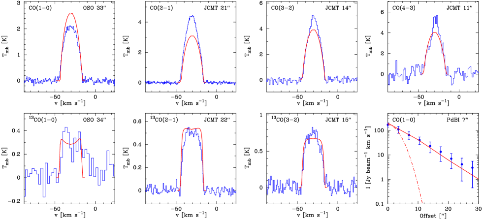
Figure 3: Multi-transition CO millimetre-wave line emission observed towards AFGL 3068. The observed spectra (histograms) have been overlayed with the best fit model results (solid lines). Also shown, lower right panel, is the observed radial brightness distribution (boxes with error bars) overlayed by the results from the model (full line), with the circular beam used in the radiative transfer analysis (dot-dashed line). The transition, telescope used, and the corresponding beamsize, are indicated for each observation.

4.3 The mass-loss rates

The determination of accurate mass-loss rates for some of these carbon stars is, it turns out, difficult in models where CO cooling is treated in a self-consistent manner (Sahai 1990; Kastner 1992; Schöier & Olofsson 2001). The reason for this is that an increase in $\dot{M}$ leads to more net cooling than heating, which compensates for the increase in molecular density, making it hard to simultaneously constrain both $\dot{M}$ and the $h$-parameter. For the sources CIT 6, IRC+10216 and IRAS 15194–5115, where a significant number of high-$J$ transitions were observed by ISO, the degeneracy between $\dot{M}$ and the $h$-parameter is partly lifted allowing for better constraints to be put on these parameters (Schöier et al. 2002). For these three sources the mass-loss rate is estimated to be accurate to about 50% within the adopted circumstellar model. For the remaining sources the uncertainty in the derived mass-loss rate is larger due to either the above mentioned degeneracy (AFGL 3068 and IRC+40540) or that only two ¹²CO lines are used in the analysis (IRAS 07454–7112 and IRAS 15082–4808). Radiative transfer analysis of the observed continuum emission from these sources (Schöier et al., in prep) give mass-loss rates that agree within $\sim$50% when compared with those derived from the CO modelling. This is reassuring and lends further credibility to the mass-loss rates presented in Table 4.

The CSEs of the sample stars have similar physical properties. However, the stars presented here are losing mass at a significantly higher rate than the average carbon star: Schöier & Olofsson (2001) measure a median mass-loss rate for carbon stars of $\sim$3$\times$10^-7 M_⊙ yr^-1, based on a sample of carbon stars complete within $\sim 600$ pc from the sun. This suggests that the stars in the sample presented here are going through the super-wind phase of evolution (e.g. Vassiliadis & Wood 1993) at the end of the AGB, and will soon eject the entire stellar mantle.

4.4 CO isotopic ratios

Using the envelope parameters derived from the ¹²CO modelling, the abundance of ¹³CO and C¹⁸O was estimated using the same radiative transfer code. The derived ¹²CO/¹³CO-ratios are presented in Table 4. The best fit ¹³CO model obtained for AFGL 3068 is overlayed onto observations and presented in Fig. 3. The fits to the observed ¹³CO emission are good in all cases with $\chi^{2}_{\mathrm{red}}$$\lesssim$1. The quality of the fits further strengthen the adopted physical models for the envelopes. The ¹²CO/¹³CO-ratio derived in this manner allows the assumption of optically thin emission adopted in Sect. 5 to be tested for those molecular species where the isotopomer containing ¹³C has been detected. All the sample stars, except for IRAS 15194–5115 (to be discussed in Sect. 6.2), have inferred ¹²C/¹³C-ratios in the range $\sim 20-50$. For optically bright carbon stars, i.e. generally lower mass-loss rate objects, values between $\sim 20-90$ are found (e.g., Schöier & Olofsson 2000; Abia et al. 2001). The observed ¹²C/¹³C-ratios are in agreement with evolutionary scenarios where the ¹²C/¹³C-ratio is thought to increase from an initial low value of $\sim 10-25$, that depends on stellar mass, as the star evolves along the AGB (Abia et al. 2001). The thermal pulses that an AGB star experiences will effectively dredge nucleosynthesized ¹²C to the surface (Iben & Renzini 1983) and, in addition to increasing the ¹²C/¹³C-ratio, eventually turn it into a carbon star with C/O$>$$1$ in its atmosphere.

C¹⁸O emission was only detected towards IRC+10216 and a C¹⁶O/C¹⁸O-ratio of 1050 is derived, using four observational constraints (including three different transitions $J$=1–0, 2–1, 3–2) for C¹⁸O. This value is in excellent agreement with the ¹⁶O/¹⁸O-ratio of 1260 obtained by Kahane et al. (1992), using a combination of optically thin emission lines. In comparison, the value of this ratio in the solar neighbourhood is around 500. The ¹⁶O/¹⁸O-ratio and in particular the ¹⁷O/¹⁸O-ratio, which is not measured here, can be used as tracers of nucleosynthesis. Like the ¹²C/¹³C-ratio, these ratios are thought to increase as the star evolves along the AGB. Kahane et al. (1992) indeed find support for this scenario in a small sample of carbon-rich evolved stars.

5 Abundance calculations

A full radiative transfer analysis of the wealth of molecular data presented here is beyond the scope of this paper. A detailed treatment of the excitation would have to include the effects of dust emission and absorption in addition to accurate rates for collisional excitation of the molecules. Instead, abundances have been calculated for species with emission that is expected to be optically thin. In the case that the emission is optically thick, the calculated abundances using this assumption will be lower limits.

The calculation of isotope ratios of various species (as shown in Table 8) shows in general that many lines are optically thick (i.e., the ratio derived from observations is lower than the ¹²CO/¹³CO abundance ratio derived from the radiative transfer analysis). Where this is the case, the abundance of the main isotope (viz., CN, CS and HC₃N) has been calculated by scaling the abundance of the less abundant isotope by the ¹²CO/¹³CO-ratio. This is indicated by the bold-faced type in Table 7. The abundance of HCN is not calculated using Eq. 3 since the line is certainly optically thick, but in all cases only by scaling the abundance of H¹³CN by the calculated ¹²CO/¹³CO-ratio.

5.1 Radiative transfer

In the calculation of molecular abundances the circumstellar envelope is assumed to have been formed by a constant mass-loss rate and to expand with a constant velocity, such that the total density distribution follows an $r^{-2}$ law. It is further assumed that the fractional abundance of a species is constant in the radial range $r_{\mathrm{i}}$ to $r_{\mathrm{e}}$ and zero outside it. The excitation temperature was assumed to be constant throughout the emitting region. With these assumptions Olofsson et al. (1990) showed that for a given molecular transition,

$$\int T_{\mathrm{mb}}{\mathrm{d}}v =\frac{c^{2}}{2k\nu^{2}}\left[B_{\nu}(T_{\mathrm{ex}})-B_{\nu}(T_{\mathrm{bg}})\right]\times$$ (3)

$$\times\ \frac{g_{u}A_{ul}}{8\pi}\frac{c^{3}}{\nu^{3}}\frac{(1-e^{-h\nu/kT_{\mathrm{ex}}})}{Z}e^{-E_{l}/kT_{\mathrm{ex}}}\times$$

$$\times\ \frac{f_{\mathrm{X}}\dot{M}_{\mathrm{H_{2}}}}{v_{\mathrm{exp}}m_{\mathrm{H_{2}}}BD}\int_{x_{\mathrm{i}}}^{x_{\mathrm{e}}}e^{-4{\ln(2)}x^{2}}{\mathrm{d}}x,$$

where $c$ is the speed of light, $h$ the Planck constant, $k$ the Boltzmann constant, $B_{\nu}$ the Planck function, $T_{\mathrm{ex}}$ the excitation temperature, $T_{\mathrm{bg}}$ is taken to be the blackbody temperature of the cosmic background radiation at 2.7 K, $m_{\mathrm{H_{2}}}$ is the mass of an H₂ molecule, $v_{\mathrm{exp}}$ the expansion velocity of the circumstellar envelope, $B$ the FWHM of the telescope beam, $D$ the assumed distance, $\dot{M}_{\mathrm{H_{2}}}$ the mass-loss rate, $Z$ the partition function, $\nu$ the frequency of the line, $g_{\mathrm{u}}$ the statistical weight of the upper level, $A_{\mathrm{ul}}$ the Einstein coefficient for the transition, $E_{\mathrm{l}}$ the energy of the lower transition level, and $x_{\mathrm{i,e}}=r_{\mathrm{i,e}}/BD$. The integral over $x$ takes care of the beam filling. However, if $r\ll BD$, the integral can be simplified to $(r_{\mathrm{e}}-r_{\mathrm{i}})/BD$. This is the case in the furthest sources, IRAS 07454–7112, CIT 6 and IRAS 15082–4808. However, for the CN emission from these sources, which tends to be very extended, and for the remaining four sources, the full integral is calculated.

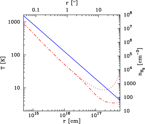
Figure 4: The density (solid line) and kinetic temperature (dotted line) structures obtained from the CO excitation analysis for AFGL 3068. Also shown is the excitation temperature of the CO($J$=2–1) line (dash-dotted line).

Table 5: Rotation temperatures

Source		13CO		CN		CS		C3N		C4H		HCN
		2–1/1–0		2–1/1–0		5–4/2–1		11–10/10–9		10–9/9–8		3–2/2–1
IRAS 07454–7112		7.0		5.2		11.3		—		—		5.7
IRC+10216 (S)		6.3		3.9		13.7		17.9		5.3		7.8
IRAS15082–4808		6.5		3.6		08.3		—		—		5.6
IRAS15194–5115		5.6		4.0		09.7		—		—		9.7
Average		6.4		4.2		10.8		17.9		5.3		7.2
Source		H(13)C3N		HC3N		HC5N		SiC2		SiS
		12–11/10–9		12–11/10–9		34–33/32–31		5-4/4-3		6–5/5–4		Average
IRAS07454–7112		08.5		15.2		—		—		05.7		08.4
IRC+10216 (S)		17.8		10.7		10.0		11.6		05.8		10.1
IRC+10216 (O)		—		—		—		—		11.8		11.8
IRAS15082–4808		—		08.9		—		37.1		05.0		10.7
IRAS15194–5115		07.2		11.3		—		—		06.1		07.7
IRC+40540		—		—		—		—		03.5		03.5
Average		11.2		11.5		10.0		24.4		06.3		08.7

5.2 The excitation temperature

Of importance in the radiative transfer analysis is the excitation (rotational) temperature assumed for the molecular emission. In Fig. 4 the kinetic temperature and density structures for AFGL 3068 are shown. In the region where most of the molecular emission observed is thought to emanate from, $\sim 10^{16}-10^{17}$ cm, the kinetic temperature ranges from $\sim 30-10$ K. Thus, if the emission were to be fully thermalized, then excitation temperatures would be expected to lie within this range. However, in addition to the low temperatures, the relatively low densities in this region, $\sim 10^{2}-10^{5}$ cm^-3, makes the CO emission partly sub-thermally excited as illustrated in Fig. 4. Thus, sub-thermal emission is to be expected for all molecular species and the excitation temperature will depend on the species (and transition) observed.

When two or more transitions of the same molecule are observed, it is possible to make an estimate of the rotation temperature ($T_{\mathrm{rot}}$) of that molecule using Eq. 3. Assuming a molecular species to be excited over the same radial range, and according to a single temperature, the rotational temperature can be estimated. The results are shown in Table 5. It is clear that the rotational temperatures vary from source to source and between molecular species in the range $\sim 3-30$ K, as to be expected. The average excitation temperature is 8.7 K (averaged over the individual excitation temperatures for all sources, rather than molecular species). A generic value of 10 K was assumed for all the abundances estimated.

5.3 The partition function

All molecules are assumed to be linear, rigid rotators, except for SiC₂ and C₃H₂ which are asymmetric tops and CH₃CN, which is a prolate symmetric top. Einstein A-coefficients (where available) and energy levels are taken from Chandra & Rashmi (1998) for SiC₂ , from Vrtilek et al. (1987) for C₃H₂, and from Boucher et al. (1980) for CH₃CN.

The partition function, $Z$, is calculated assuming that no molecules have a hyperfine structure, i.e. as having simple rotational energy diagrams. Hence the integrated intensities which are summed over all hyperfine components are used. For C₃H₂, CH₃CN and SiC₂ we use the approximate expression for an asymmetric rotor (Townes & Schawlow 1975) multiplied by 2 for C₃H₂, by 4 for CH₃CN (to account for spin statistics) and by 1/2 for SiC₂ (since half of the energy levels are missing because of spin statistics). It is assumed that all levels are populated according to $T_{\mathrm{ex}}$.

5.4 Sizes of emission regions

5.4.1 Photodissociation radii

The chemical richness observed towards carbon stars can be qualitatively understood in terms of a photodissociation model (see the review by Glassgold 1996). Carbon-bearing molecules like CO, C₂H₂, HCN and CS, in addition to Si-bearing molecules like SiS and SiO, are all thought to be of photospheric origin where they are formed in conditions close to LTE. The photodissociation of these so-called parent species produces various radicals and ions that, in turn, drive a complex chemistry through ion-molecule and neutral-neutral reactions. For example, the radicals C₂H and CN are the photodissociation products of C₂H₂ and HCN, respectively. In addition, the formation of dust in the CSE will affect the abundances of some of the species, in particular SiO and SiS, which condense onto dust grains. All other species observed in the sample are thought to be products of the circumstellar chemistry.

Table 6: Photodissociation rates

Molecule	$G_{0}$
	[s-1]
HCN	1.1 10${}^{-9\phantom{0}}$
CN	2.5 10-10
C2H2	2.1 10${}^{-9\phantom{0}}$
C2H	3.4 10-10
SiS	6.3 10-10
CS	6.3 10-10
SiO	6.3 10-10

To calculate the radial extent of the molecules HCN, CN, C₂H and CS the photodissociation model of Huggins & Glassgold (1982) is adopted. The photodissociation radius of a parent species ($f_{\mathrm{X}}$, viz., HCN, C₂H₂, CS) is determined by

$$\frac{{\mathrm{d}}f_{\mathrm{X}}}{{\mathrm{d}}r}=-\frac{G_{\mathrm{0,X}}}{v_{\mathrm{exp}}}{\mathrm{e}}^{-d_{\mathrm{X}}/r}f_{\mathrm{X}}$$ (4)

and of a daughter ($f_{\mathrm{Xd}}$, viz., C₂H) by

$$\frac{{\mathrm{d}}f_{\mathrm{Xd}}}{{\mathrm{d}}r}=\frac{G_{\mathrm{0,X}}}{v_{\mathrm{exp}}}{\mathrm{e}}^{-d_{\mathrm{X}}/r}f_{\mathrm{X}}-\frac{G_{\mathrm{0,Xd}}}{v_{\mathrm{exp}}}{\mathrm{e}}^{-d_{\mathrm{Xd}}/r}f_{\mathrm{Xd}}$$ (5)

$G_{0}$ is the unshielded photodissociation rate and $d_{\mathrm{X}}$ is the dust shielding distance, given by:

$$d_{\mathrm{X}}=1.4\frac{3Q_{\mathrm{X}}}{4a_{\mathrm{d}}\rho_{\mathrm{d}}}\frac{\dot{M}_{\mathrm{d}}}{4\pi v_{\mathrm{d}}},$$ (6)

where $Q$ is the dust absorption efficiency, $\dot{M}_{\mathrm{d}}$ the dust mass-loss rate, and $v_{\mathrm{d}}$ the expansion velocity of the dust grains (Jura & Morris 1981). Since different molecules are generally dissociated at different wavelengths the adopted value of $Q$ will depend on the species under study. However, the wavelength dependence of $Q$ in the region of interest, $\sim$1000–3000 Å, is weak (e.g., Suh 2000) and a generic value of 1.0 for most species of interest here is adopted. However, the shielding distance of CN is taken to be a factor of 1.2 greater than that used for HCN (Truong-Bach et al. 1987). Introducing the $h$-parameter defined in Eq. 2 the dust shielding distance may now be expressed as

$$d=5.27\,10^{22}\,\frac{h\dot{M}}{v_{\mathrm{d}}}\quad{\mathrm{cm}},$$ (7)

where the H₂ mass-loss rate $\dot{M}$ is given in M_⊙ yr^-1 and $v_{\mathrm{d}}$ in ${\mathrm{km\,s}}^{-1}$. A gas-to-dust mass ratio of 0.01 was assumed.

There will generally be a drift velocity between the dust and the gas (e.g., Schöier & Olofsson 2001)

$$v_{\mathrm{d}}-v_{\mathrm{exp}}=\sqrt{\frac{Lv_{\mathrm{exp}}\langle Q\rangle}{\dot{M}c}},$$ (8)

where $L$ is the bolometric luminosity of the star, $c$ the speed of light, and $\langle Q\rangle$ is the flux-averaged momentum transfer efficiency. The drift velocity also enters in the expression of the heating caused by dust-gas collisions. In the self-consistent treatment of the energy balance in the circumstellar envelope a value of 0.03 was assumed for $\langle Q\rangle$, which is also retained here. Photodissocation rates are taken from van Dishoeck (1988), with the assumption that SiS has the same photodissociation rate as CS (confirmed to within a factor 2 by the UMIST Ratefile). The calculated shielding distances and rate coefficients are shown in Tables 4 and 6, respectively.

Table 7: Abundances and sizes of emission regions^a

Molecule	IRC+10216 (SEST)				IRC+10216 (OSO)				IRAS15194-5115				IRAS15082-4808
	$r_{\rm i}$	$r_{\rm e}$	$f_{\rm X}$		$r_{\rm i}$	$r_{\rm e}$	$f_{\rm X}$		$r_{\rm i}$	$r_{\rm e}$	$f_{\rm X}$		$r_{\rm i}$	$r_{\rm e}$	$f_{\rm X}$
	[cm]	[cm]	[X]/[H2]		[cm]	[cm]	[X]/[H2]		[cm]	[cm]	[X]/[H2]		[cm]	[cm]	[X]/[H2]
CN(1–0)	2.6 (16)	7.1 (16)	3.4 (-06)		2.6 (16)	7.1 (16)	2.1 (-06)		3.5 (16)	9.6 (16)	2.1 (-06)		2.0 (16)	6.2 (16)	3.2 (-06)
13CN(1–0)	2.6 (16)	7.1 (16)	7.6 (-08)		2.6 (16)	7.1 (16)	4.6 (-08)		3.5 (16)	9.6 (16)	3.0 (-07)		2.0 (16)	6.2 (16)	$<$ 1.3 (-08)
CN(2–1)	2.6 (16)	7.1 (16)	9.6 (-07)		2.6 (16)	7.1 (16)	—		3.5 (16)	9.6 (16)	3.5 (-07)		2.0 (16)	6.2 (16)	3.8 (-07)
CS(2–1)		4.0 (16)	9.9 (-07)			4.0 (16)	4.6 (-07)			5.5 (16)	2.3 (-06)			3.3 (16)	2.2 (-06)
13CS(2–1)		4.0 (16)	2.2 (-08)			4.0 (16)	—			5.5 (16)	5.0 (-07)			3.3 (16)	$<$ 3.1 (-08)
C34S(2–1)		4.0 (16)	3.7 (-08)			4.0 (16)	—			5.5 (16)	—			3.3 (16)	—
CS(5–4)		4.0 (16)	1.2 (-06)			4.0 (16)	—			5.5 (16)	1.6 (-06)			3.3 (16)	9.0 (-07)
C2S(6,7–5,6)	1.2 (16)	4.0 (16)	$<$ 4.6 (-09)		1.2 (16)	4.0 (16)	$<$ 4.5 (-09)		8.0 (15)	5.5 (16)	$<$ 2.4 (-08)		7.4 (15)	3.3 (16)	$<$ 3.1 (-08)
C2S(8,9–7,8)	1.2 (16)	4.0 (16)	$<$ 4.1 (-09)		1.2 (16)	4.0 (16)	$<$ 9.5 (-09)		8.0 (15)	5.5 (16)	$<$ 3.5 (-08)		7.4 (15)	3.3 (16)	$<$ 4.8 (-08)
C3S(15-14)	1.2 (16)	4.0 (16)	$<$ 1.2 (-08)		1.2 (16)	4.0 (16)	$<$ 1.5 (-08)		8.0 (15)	5.5 (16)	$<$ 7.2 (-08)		7.4 (15)	3.3 (16)	$<$ 1.3 (-06)
SiO(2–1)		2.0 (16)	1.3 (-07)			2.0 (16)	9.6 (-08)			1.3 (16)	1.7 (-06)			3.3 (16)	7.2 (-07)
SiS(5–4)		2.0 (16)	1.2 (-06)			2.0 (16)	8.1 (-07)			1.3 (16)	4.9 (-06)			3.3 (16)	3.3 (-06)
SiS(6–5)		2.0 (16)	9.0 (-07)			2.0 (16)	9.0 (-07)			1.3 (16)	4.2 (-06)			3.3 (16)	2.0 (-06)
SO(3–2)	2.6 (16)	7.1 (16)	$<$ 3.5 (-09)		2.6 (16)	7.1 (16)	—		3.5 (16)	9.6 (16)	—		2.0 (16)	6.2 (16)	—
HCN(1–0)		3.4 (16)	1.4 (-05)			3.4 (16)	1.1 (-05)			4.6 (16)	1.2 (-05)			2.7 (16)	1.0 (-05)
H13CN(1–0)		3.4 (16)	3.1 (-07)			3.4 (16)	2.5 (-07)			4.6 (16)	2.0 (-06)			2.7 (16)	2.9 (-07)
HNC(1–0)	2.4 (16)	8.4 (16)	7.2 (-08)		2.4 (16)	8.4 (16)	3.8 (-08)		1.6 (16)	5.6 (16)	3.3 (-07)		1.5 (16)	5.2 (16)	1.6 (-07)
HN13C(1–0)	2.4 (16)	8.4 (16)	$<$ 1.9 (-09)		2.4 (16)	8.4 (16)	—		1.6 (16)	5.6 (16)	1.1 (-07)		1.5 (16)	5.2 (16)	$<$ 1.2 (-08)
SiC2(4,04–3,03)	2.4 (16)	6.0 (16)	1.6 (-07)		2.4 (16)	6.0 (16)	—		1.6 (16)	4.0 (16)	—		1.5 (16)	3.7 (16)	3.3 (-07)
SiC2(4,22–3,21)	2.4 (16)	6.0 (16)	3.2 (-07)		2.4 (16)	6.0 (16)	—		1.6 (16)	4.0 (16)	—		1.5 (16)	3.7 (16)	$<$ 1.8 (-07)
SiC2(5,05–4,04)	2.4 (16)	6.0 (16)	1.7 (-07)		2.4 (16)	6.0 (16)	1.7 (-07)		1.6 (16)	4.0 (16)	1.2 (-06)		1.5 (16)	3.7 (16)	4.9 (-07)
C2H(1–0)	2.3 (16)	5.6 (16)	2.8 (-06)		2.3 (16)	5.6 (16)	2.4 (-06)		1.6 (16)	4.8 (16)	1.5 (-05)		1.7 (16)	4.8 (16)	8.3 (-06)
C3H(9/2–7/2)	2.4 (16)	8.4 (16)	5.5 (-08)		2.4 (16)	8.4 (16)	5.9 (-08)		1.6 (16)	5.6 (16)	9.2 (-08)		1.5 (16)	5.2 (16)	$<$ 1.7 (-08)
C3N(9–8)	2.4 (16)	8.4 (16)	3.0 (-07)		2.4 (16)	8.4 (16)	—		1.6 (16)	5.6 (16)	$<$ 4.9 (-08)		1.5 (16)	5.2 (16)	$<$ 1.0 (-07)
C3N(11–10)	2.4 (16)	8.4 (16)	5.9 (-07)		2.4 (16)	8.4 (16)	7.6 (-07)		1.6 (16)	5.6 (16)	9.2 (-07)		1.5 (16)	5.2 (16)	9.5 (-07)
C4H(9–8)	2.4 (16)	8.4 (16)	3.7 (-06)		2.4 (16)	8.4 (16)	—		1.6 (16)	5.6 (16)	—		1.5 (16)	5.2 (16)	$<$ 6.6 (-07)
C4H(10–9)	2.4 (16)	8.4 (16)	2.7 (-06)		2.4 (16)	8.4 (16)	3.2 (-06)		1.6 (16)	5.6 (16)	2.8 (-05)		1.5 (16)	5.2 (16)	6.9 (-06)
C3H2(2,12–1,01)	2.4 (16)	8.4 (16)	3.2 (-08)		2.4 (16)	8.4 (16)	—		1.6 (16)	5.6 (16)	6.0 (-07)		1.5 (16)	5.2 (16)	$<$ 9.3 (-08)
HC3N(10–9)	1.2 (16)	6.0 (16)	1.1 (-06)		1.2 (16)	6.0 (16)	4.4 (-07)		8.0 (15)	4.0 (16)	1.9 (-06)		7.4 (15)	3.7 (16)	2.3 (-06)
HCC13CN(10–9)	1.2 (16)	6.0 (16)	2.4 (-08)		1.2 (16)	6.0 (16)	$<$ 2.8 (-09)		8.0 (15)	4.0 (16)	3.9 (-07)		7.4 (15)	3.7 (16)	$<$ 2.7 (-08)
HC13CCN(10–9)	1.2 (16)	6.0 (16)	2.4 (-08)		1.2 (16)	6.0 (16)	$<$ 2.8 (-09)		8.0 (15)	4.0 (16)	3.9 (-07)		7.4 (15)	3.7 (16)	$<$ 2.7 (-08)
HC3N(11–10)	1.2 (16)	6.0 (16)	7.5 (-07)		1.2 (16)	6.0 (16)	—		8.0 (15)	4.0 (16)	—		7.4 (15)	3.7 (16)	—
HC3N(12–11)	1.2 (16)	6.0 (16)	1.9 (-06)		1.2 (16)	6.0 (16)	—		8.0 (15)	4.0 (16)	2.2 (-06)		7.4 (15)	3.7 (16)	2.1 (-06)
HCC13CN(12–11)	1.2 (16)	6.0 (16)	4.1 (-08)		1.2 (16)	6.0 (16)	1.5 (-08)		8.0 (15)	4.0 (16)	2.8 (-07)		7.4 (15)	3.7 (16)	$<$ 2.0 (-08)
HC13CCN(12–11)	1.2 (16)	6.0 (16)	4.1 (-08)		1.2 (16)	6.0 (16)	1.5 (-08)		8.0 (15)	4.0 (16)	2.8 (-07)		7.4 (15)	3.7 (16)	$<$ 2.0 (-08)
CH3CN(6(1)–5(1))	1.2 (16)	6.0 (16)	1.2 (-08)		1.2 (16)	6.0 (16)	$<$ 2.0 (-09)		8.0 (15)	4.0 (16)	$<$ 2.5 (-08)		7.4 (15)	3.7 (16)	$<$ 4.3 (-08)
CH3CN(12(0)–11(0))	1.2 (16)	6.0 (16)	$<$ 1.2 (-07)		1.2 (16)	6.0 (16)	—		8.0 (15)	4.0 (16)	$<$ 2.4 (-06)		7.4 (15)	3.7 (16)	$<$ 1.5 (-06)
HC5N(32–31)	1.2 (16)	6.0 (16)	3.9 (-06)		1.2 (16)	6.0 (16)	—		8.0 (15)	4.0 (16)	$<$ 4.5 (-06)		7.4 (15)	3.7 (16)	$<$ 3.8 (-06)
HC5N(34–33)	1.2 (16)	6.0 (16)	4.2 (-06)		1.2 (16)	6.0 (16)	$<$ 7.6 (-07)		8.0 (15)	4.0 (16)	—		7.4 (15)	3.7 (16)	$<$ 7.4 (-06)
HC5N(35–34)	1.2 (16)	6.0 (16)	1.3 (-05)		1.2 (16)	6.0 (16)	—		8.0 (15)	4.0 (16)	—		7.4 (15)	3.7 (16)	$<$ 1.1 (-05)

1. In this table $x\,(y)$ represents $x\times 10^{y}$.

2. Bold face indicates an abundance calculated by scaling the abundance of the ¹³C isotope of the same species by the modelled ¹²CO/¹³CO-ratio (see Sect. 5.5).

Table 7: (cont.) Abundances and sizes of emission regions^a

Molecule	IRAS07454-7112				CIT 6				AFGL 3068				IRC+40540
	$r_{\rm i}$	$r_{\rm e}$	$f_{\rm X}$		$r_{\rm i}$	$r_{\rm e}$	$f_{\rm X}$		$r_{\rm i}$	$r_{\rm e}$	$f_{\rm X}$		$r_{\rm i}$	$r_{\rm e}$	$f_{\rm X}$
	cm	cm	[X]/[H2]		cm	cm	[X]/[H2]		cm	cm	[X]/[H2]		cm	cm	[X]/[H2]
CN(1–0)	1.3 (16)	4.1 (16)	5.3 (-06)		1.6 (16)	5.1 (16)	2.0 (-05)		3.2 (16)	8.3 (16)	4.6 (-07)		3.2 (16)	8.3 (16)	1.0 (-06)
13CN(1–0)	1.3 (16)	4.1 (16)	4.8 (-07)		1.6 (16)	5.1 (16)	5.8 (-07)		3.2 (16)	8.3 (16)	$<$ 2.6 (-08)		3.2 (16)	8.3 (16)	$<$ 9.9 (-09)
CN(2–1)	1.3 (16)	4.1 (16)	1.6 (-06)		1.6 (16)	5.1 (16)	—		3.2 (16)	8.3 (16)	—		3.2 (16)	8.3 (16)	—
CS(2–1)		2.2 (16)	1.6 (-06)			2.7 (16)	2.5 (-06)			4.8 (16)	3.7 (-07)			4.9 (16)	5.4 (-07)
13CS(2–1)		2.2 (16)	$<$ 2.9 (-08)			2.7 (16)	—			4.8 (16)	—			4.9 (16)	—
C34S (2–1)		2.2 (16)	—			2.7 (16)	—			4.8 (16)	—			4.9 (16)	—
CS(5–4)		2.2 (16)	1.6 (-06)			2.7 (16)	—			4.8 (16)	—			4.9 (16)	—
C2S(6,7–5,6)	5.6 (15)	2.2 (16)	$<$ 9.1 (-08)		4.3 (15)	2.7 (16)	$<$ 1.0 (-07)		1.6 (16)	4.8 (16)	$<$ 8.1 (-08)		1.6 (16)	4.9 (16)	$<$ 3.0 (-08)
C2S(8,9–7,8)	5.6 (15)	2.2 (16)	$<$ 1.1 (-07)		4.3 (15)	2.7 (16)	$<$ 2.0 (-07)		1.6 (16)	4.8 (16)	$<$ 8.0 (-08)		1.6 (16)	4.9 (16)	$<$ 5.6 (-08)
C3S(15-14)	5.6 (15)	2.2 (16)	$<$ 3.6 (-07)		4.3 (15)	2.7 (16)	$<$ 2.5 (-07)		1.6 (16)	4.8 (16)	$<$ 3.5 (-07)		1.6 (16)	4.9 (16)	$<$ 8.9 (-08)
SiO(2–1)		9.4 (15)	4.4 (-07)			7.2 (15)	1.0 (-06)			2.6 (16)	$<$ 4.7 (-08)			2.6 (16)	5.6 (-08)
SiS(5–4)		9.4 (15)	4.8 (-06)			7.2 (15)	1.0 (-06)			2.6 (16)	3.3 (-07)			2.6 (16)	1.4 (-06)
SiS(6–5)		9.4 (15)	3.4 (-06)			7.2 (15)	5.2 (-06)			2.6 (16)	1.0 (-06)			2.6 (16)	4.9 (-07)
HCN(1–0)		1.8 (16)	7.8 (-06)			2.2 (16)	1.1 (-05)			4.2 (16)	6.3 (-06)			4.2 (16)	6.5 (-06)
H13CN(1–0)		1.8 (16)	5.6 (-07)			2.2 (16)	3.0 (-07)			4.2 (16)	2.1 (-07)			4.2 (16)	1.3 (-07)
HNC(1–0)	1.1 (16)	4.0 (16)	1.0 (-07)		8.6 (15)	3.0 (16)	2.3 (-07)		3.1 (16)	1.1 (17)	3.0 (-08)		3.1 (16)	1.1 (17)	2.2 (-08)
HN13C(1–0)	1.1 (16)	4.0 (16)	$<$ 1.8 (-08)		8.6 (15)	3.0 (16)	$<$ 2.1 (-08)		3.1 (16)	1.1 (17)	$<$ 1.4 (-08)		3.1 (16)	1.1 (17)	$<$ 4.4 (-09)
SiC2(4,04–3,03)	1.1 (16)	2.8 (16)	2.3 (-07)		8.6 (15)	2.2 (16)	—		3.1 (16)	7.8 (16)	—		3.1 (16)	7.8 (16)	—
SiC2(4,22–3,21)	1.1 (16)	2.8 (16)	$<$ 2.7 (-07)		8.6 (15)	2.2 (16)	—		3.1 (16)	7.8 (16)	—		3.1 (16)	7.8 (16)	—
SiC2(5,05–4,04)	1.1 (16)	2.8 (16)	$<$ 3.2 (-07)		8.6 (15)	2.2 (16)	3.1 (-06)		3.1 (16)	7.8 (16)	$<$ 7.5 (-08)		3.1 (16)	7.8 (16)	$<$ 5.3 (-08)
C2H(1–0)	1.1 (16)	3.2 (16)	$<$ 4.3 (-07)		1.4 (16)	4.1 (16)	6.9 (-06)		2.8 (16)	6.7 (16)	5.7 (-06)		2.7 (16)	6.7 (16)	$<$ 1.0 (-07)
C3H(9/2–7/2)	1.1 (16)	4.0 (16)	$<$ 3.1 (-08)		8.6 (15)	3.0 (16)	$<$ 7.4 (-08)		3.1 (16)	1.1 (17)	$<$ 1.4 (-08)		3.1 (16)	1.1 (17)	$<$ 1.2 (-08)
C3N(9–8)	1.1 (16)	4.0 (16)	$<$ 1.6 (-07)		8.6 (15)	3.0 (16)	—		3.1 (16)	1.1 (17)	—		3.1 (16)	1.1 (17)	—
C3N(11–10)	1.1 (16)	4.0 (16)	7.3 (-07)		8.6 (15)	3.0 (16)	2.6 (-06)		3.1 (16)	1.1 (17)	5.5 (-07)		3.1 (16)	1.1 (17)	1.1 (-07)
C4H(9–8)	1.1 (16)	4.0 (16)	—		8.6 (15)	3.0 (16)	—		3.1 (16)	1.1 (17)	—		3.1 (16)	1.1 (17)	—
C4H(10–9)	1.1 (16)	4.0 (16)	$<$ 8.8 (-07)		8.6 (15)	3.0 (16)	$<$ 1.7 (-06)		3.1 (16)	1.1 (17)	—		3.1 (16)	1.1 (17)	—
C3H2(2,12–1,01)	1.1 (16)	4.0 (16)	—		8.6 (15)	3.0 (16)	—		3.1 (16)	1.1 (17)	—		3.1 (16)	1.1 (17)	—
HC3N(10–9)	5.6 (15)	2.8 (16)	1.7 (-06)		4.3 (15)	2.2 (16)	2.4 (-06)		1.6 (16)	7.8 (16)	5.0 (-07)		1.6 (16)	7.8 (16)	1.5 (-06)
HCC13CN(10–9)	5.6 (15)	2.8 (16)	1.5 (-07)		4.3 (15)	2.2 (16)	$<$ 4.9 (-08)		1.6 (16)	7.8 (16)	$<$ 1.5 (-08)		1.6 (16)	7.8 (16)	3.1 (-08)
HC13CCN(10–9)	5.6 (15)	2.8 (16)	1.5 (-07)		4.3 (15)	2.2 (16)	$<$ 4.9 (-08)		1.6 (16)	7.8 (16)	$<$ 1.5 (-08)		1.6 (16)	7.8 (16)	3.1 (-08)
HC3N(11–10)	5.6 (15)	2.8 (16)	—		4.3 (15)	2.2 (16)	—		1.6 (16)	7.8 (16)	—		1.6 (16)	7.8 (16)	—
HC3N(12–11)	5.6 (15)	2.8 (16)	2.4 (-06)		4.3 (15)	2.2 (16)	—		1.6 (16)	7.8 (16)	—		1.6 (16)	7.8 (16)	—
HCC13CN(12–11)	5.6 (15)	2.8 (16)	1.3 (-07)		4.3 (15)	2.2 (16)	2.7 (-07)		1.6 (16)	7.8 (16)	$<$ 2.9 (-08)		1.6 (16)	7.8 (16)	$<$ 1.1 (-08)
HC13CCN(12–11)	5.6 (15)	2.8 (16)	1.3 (-07)		4.3 (15)	2.2 (16)	2.7 (-07)		1.6 (16)	7.8 (16)	$<$ 2.9 (-08)		1.6 (16)	7.8 (16)	$<$ 1.1 (-08)
CH3CN(6(1)–5(1))	5.6 (15)	2.8 (16)	$<$ 2.4 (-07)		4.3 (15)	2.2 (16)	$<$ 1.3 (-07)		1.6 (16)	7.8 (16)	$<$ 1.2 (-07)		1.6 (16)	7.8 (16)	$<$ 6.4 (-08)
CH3CN(12(0)–11(0))	5.6 (15)	2.8 (16)	$<$ 4.6 (-06)		4.3 (15)	2.2 (16)	—		1.6 (16)	7.8 (16)	—		1.6 (16)	7.8 (16)	—
HC5N(32–31)	5.6 (15)	2.8 (16)	—		4.3 (15)	2.2 (16)	—		1.6 (16)	7.8 (16)	—		1.6 (16)	7.8 (16)	—
HC5N(34–33)	5.6 (15)	2.8 (16)	9.2 (-06)		4.3 (15)	2.2 (16)	$<$ 1.3 (-05)		1.6 (16)	7.8 (16)	$<$ 4.1 (-06)		1.6 (16)	7.8 (16)	$<$ 4.5 (-06)
HC5N(35–34)	5.6 (15)	2.8 (16)	$<$ 8.8 (-06)		4.3 (15)	2.2 (16)	—		1.6 (16)	7.8 (16)	—		1.6 (16)	7.8 (16)	—

1. In this table $x\,(y)$ represents $x\times 10^{y}$.

2. Bold face indicates an abundance calculated by scaling the abundance of the ¹³C isotope of the same species by the modelled ¹²CO/¹³CO-ratio (see Sect. 5.5).

The photodissociation radii of species formed in the photosphere were chosen to be the e–folding radii of the initial abundances, i.e. $f_{\mathrm{X}}(r_{\mathrm{e}})=f_{\mathrm{X}}(R_{\star})/{\mathrm{e}}$, where $R_{\star}$ is the stellar radius. For the photodissociation products inner and outer radii are chosen to be where the abundance has dropped to 1/e of its peak value. The envelope sizes calculated by the simple photodissociation model agree relatively well with observed values in IRC+10216 and other objects, except in the case of SiS (see next paragraph). Lindqvist et al. (2000) used a detailed radiative transfer method and observed brightness distributions to derive envelope sizes of HCN and CN. For IRC+10216 and IRC+40540 they found envelope sizes of $\sim$4$\times$10¹⁶ cm for HCN and $\sim$5$\times$10¹⁶ cm for CN, in excellent agreement with the values derived here from the photodissociation model. In the case of CIT 6 the observed HCN envelope size is larger than that calculated by a factor of 2. Envelope sizes and derived abundances are given in Table 7.

SiO and SiS are parent species with a radial extent depending on photodissociation. The calculation of the SiS photodissociation radius in IRC+10216, however, is not consistent with the radius observed by Bieging & Tafalla (1993). Therefore the observed radius for SiS in IRC+10216 was used in the abundance calculations, and its radius was scaled for the other objects in the sample with the factor $(\dot{M}/v_{\mathrm{exp}})_{\star}/(\dot{M}/v_{\mathrm{exp}})_{10216}$ in the same way as described in section 5.4.2. The outer radius calculated via the photodissociation model is actually slightly larger than that observed. This gives credence to the idea that SiS freezes out onto dust grains. SiO is treated in the same way as SiS since it too is likely to freeze out onto grains. Hence the same envelope size as SiS was adopted for this species.

5.4.2 Inner and outer radii for species of circumstellar chemistry origin

For those molecules that have their origin in a circumstellar chemistry a different approach is used. The sizes of the emission regions of HNC and HC₃N have been determined interferometrically for IRC+10216 using observations by Bieging & Rieu (1988), and of SiC₂ by Lucas et al. (1995). Inner and outer radii for HNC, HC₃N and SiC₂ are taken from observations of IRC+10216, and scaled by a factor $(\dot{M}/v_{\mathrm{exp}})_{\star}/(\dot{M}/v_{\mathrm{exp}})_{10216}$ for the remaining six sample carbon stars (since molecular distributions have not been mapped in all the sample stars; see Table 4 for values of this ratio). This factor is proportional to the density ratio at a given radius, and also (to the first order) to the ratio of the envelope shielding distances. Chemical modelling shows that the species C₃H, C₄H, C₃H₂, C₃N, CH₃CN, HC₅N, SO, C₂S and C₃S are formed via chemical reactions in the outer envelope (e.g., Millar & Herbst 1994). Furthermore, it shows that the species C₃H, C₄H, C₃H₂ and C₃N have a similar radial distribution to HNC, and that the species CH₃CN and HC₅N are similarly distributed to HC₃N. Hence corresponding radii for these species are assumed in the calculations. SO is assumed to have a similar distribution to CN (c.f., Nejad & Millar 1988), and C₂S and C₃S are assumed to follow the CS distribution (c.f., Millar et al. 2001), although these latter two species are not parent molecules (and hence are given an inner radius equal to that of HC₃N). All isotopes (i.e. species involving ¹³C and ³⁴S) are further assumed to have the same distributions as the main isotope.

Table 8: Molecular isotope abundance ratios

	IRC+10216 (S)	IRC+10216 (O)	IRAS15194	IRAS07454	CIT 6	IRC+40540
HC3N/HC13CCN(10–9)	32.6	—	4.9	11.1	—	17.9
HC3N/HC13CCN(12–11)	22.1	—	7.9	17.8	—	—
CS/13CS(2–1)	22.7	—	4.6	—	—	—
CN/13CN(1–0)	25.1	46.6	6.7	11.0	12.4	—
Average	25.6	46.6	6.0	13.3	12.4	17.9
Modelling of CO (Table 4)	45.0	45.0	6.0	14.0	35.0	50.0

5.5 Molecular abundances

5.5.1 Uncertainties in the abundance estimates

The assumption of optically thin emission has a systematic effect on the derived abundances, in that the true abundance will be higher if there are opacity effects. As can be seen from Table 8, there can be a factor of 2–3 in error from this assumption.

The accuracy of the calculated abundances is dependent on various assumptions. Due to the intrinsic difficulties in estimating distances to the objects included in the sample, the typical uncertainty in the adopted distance is a factor of $\sim$2. This influences the mass-loss rates derived in the radiative transfer modelling such that the adopted mass-loss rate will scale as $D^{1-2}$. The calculation of the limiting radii of a certain molecular distribution in the envelope is also affected by inaccuracies in the distance estimate. Where radii have been calculated by scaling observed radii in IRC+10216, there comes an error which scales as $D$. The results from the photodissociation model will have a lesser dependence, with $D$ coming into the expression for the shielding distance, via $\dot{M}$. Hence the abundance, which is trivially derived from Eq. 3, will vary as approximately $D^{-1-0}$, giving a factor of 2, possibly, in error.

In the present analysis an excitation temperature of 10 K was assumed for all transitions. The error in abundance estimate due to this assumption will depend on the excitation temperature of a particular transition and the assumption of LTE, and is estimated to be not more than a factor of $\sim$2.

Overall, it seems like an error of a factor of 5 is reasonable to expect in the abundances presented here, although it should be borne in mind that this could possibly rise to an order of magnitude. In the comparison of abundance ratios in Table 9, any difference less than a factor of 5 is treated as insignificant with respect to error margins.

5.5.2 Comparison with previously published abundances

In comparison with Nyman et al. (1993), derived abundance ratios (Table 9) have increased in favour of IRAS 15194–5115 by up to a factor of approximately 4. Individual abundances generally show a factor $\sim$2 increase for those in IRAS 15914–5115, and a factor $\sim$2 decrease for IRC+10216, over Nyman et al. (1993). In Nyman et al. (1993), the distances adopted for IRC+10216 and IRAS 15194-5115 were approximately twice as large as those here; however this has little effect on calculated abundances since the distance ratio is more or less unchanged. However, the calculated mass-loss rate of IRAS 15194–5115 in the previous paper was larger than that of IRC+10216 by a factor of 2.5, and here the recalculated mass-loss rates are the same for these two objects. This would tend to increase the abundance ratios quoted by a similar factor. The photodissociation radius depends on the mass-loss rate and the dust parameters through the dust shielding distance. Compared to Nyman et al. (1993) this paper uses different mass-loss rates, a different gas-to-dust ratio (0.01 compared to 0.005), and the dust parameters are also slightly different due to the determination of the $h$–factor in the radiative transfer analysis. The scale factor that determines the inner and outer radii of the species with a origin in circumstellar chemistry depends on the ratio of the mass-loss rates. Thus the difference in relative mass loss rates explains the factor of 4 difference in relative abundances between IRAS 15914–5115 and IRC+10216 derived in this paper compared to those derived in Nyman et al. (1993).

As discussed earlier in this paper the outer radii of SiS and SiO are not determined through the photodissociation radius but scaled from their observed radius in IRC+10216. In this way the calculated abundances of SiO and SiS have increased in by a factor of 4–5 for IRAS 15194–5115 compared to Nyman et al. (1993). For IRC+10216 these species have the same abundance as calculated previously, and they are in reasonable agreement with those reported elsewhere in the literature. Bujarrabal et al. (1994) give $f($SiO$)$ = 5.6 10^-7 and $f($SiS$)$ = 3.9 10^-6, which are $\sim$4 times greater, using an outer radius half that quoted in this paper and a distance of 200 pc. Better agreement is seen for the other species which Bujarrabal et al. (1994) detect, with the exception of HNC, which is a factor $\sim$6 in disagreement. Cernicharo, Guélin, & Kahane (2000) also calculate abundances in IRC+10216, and are within a factor 5 of those here.

Generally, it seems that IRC+10216 has lower abundances than IRAS 15194–5115, IRAS 15082–4808, IRAS 07454–7112 and CIT 6. However, it is very similar, physically and chemically, to AFGL 3068 and IRC+40540.

The three northern sources observed at OSO have also been studied in the literature, and abundances derived. The Bujarrabal et al. (1994) paper includes data relating to CIT 6, AFGL 3068 and IRC+40540. All abundances calculated by Bujarrabal et al. in these three sources are greater than those derived here. Distances and mass-loss rates are reasonably comparable between this paper and that. Generally, this means that the calculated abundances in this paper are lower by a factor of $\sim$2 in CIT 6, a factor of $\sim$5 in AFGL 3068, and a factor of $\sim$3 in IRC+40540 compared to those derived in Bujarrabal et al. (1994).

Table 9: Abundance ratios, compared to IRC+10216 observed with the SEST.

	IRC+10216			IRAS15194	IRAS15082	IRAS07454	00CIT 600	AFGL 3068	IRC+40540
Molecule	SEST		OSO
CN(1-0)	1.0		1.1	01.1	1.7	2.8	03.8	0.2	0.5
13CN(1-0)	1.0		0.6	04.0	—	6.3	07.6	—	—
CN(2-1)	1.0		—	00.4	0.4	1.7	—	—	—
CS(2-1)	1.0		0.9	04.6	4.3	3.2	05.1	0.7	1.1
13CS(2-1)	1.0		—	22.7	—	—	—	—	—
CS(5-4)	1.0		—	01.4	0.8	1.4	—	—	—
SiO(2-1)	1.0		0.7	12.8	5.4	3.3	07.8	—	0.4
SiS(5-4)	1.0		0.7	04.0	2.7	3.9	00.8	0.3	1.1
SiS(6-5)	1.0		1.0	04.7	2.2	3.8	05.7	1.1	0.5
HCN	1.0		0.8	00.9	0.7	0.6	00.8	0.5	0.5
H13CN(1-0)	1.0		0.8	06.4	0.9	1.8	01.0	0.7	0.4
HNC(1-0)	1.0		0.5	04.6	2.2	1.4	03.2	0.4	0.3
SiC2(4,04-3,03)	1.0		—	—	2.0	1.5	—	—	—
SiC2(5,05-4,04)	1.0		1.0	06.9	2.8	—	17.7	—	—
C2H(1-0)	1.0		0.9	05.6	3.0	—	02.5	2.0	—
C3H(9/2-7/2)	1.0		1.1	01.7	—	—	—	—	—
C3N(11-10)	1.0		1.3	01.5	1.6	1.2	04.4	0.9	0.2
C4H(10-9)	1.0		1.2	10.4	2.6	—	—	—	—
C3H2(2,12-1,01)	1.0		—	18.6	—	—	—	—	—
HC3N(10-9)	1.0		0.6	02.4	3.0	2.2	03.1	0.6	0.7
H(13)C3N(10-9)a	1.0		—	16.3	—	6.4	—	—	1.3
HC3N(12-11)	1.0		—	02.5	2.3	2.6	—	—	—
H(13)C3N(12-11)a	1.0		0.4	06.9	—	3.3	06.6	—	—
HC5N(34-33)	1.0		—	—	—	2.2	—	—	—

(a) Bold face signifies a factor of more than 5.

1. signifies blend of HCC¹³CN and HC¹³CCN.

Table 10: Fractional abundances for IRC+10216 for species of photospheric origin.

Species	Observeda		Modelb
			TE	Shock
CO	1.0(-3)c		9.8(-4)	1.0(-3)
HCN	1.3(-5)c		5.1(-5)	3.1(-6)
CS	9.9(-7)c		1.3(-5)	7.1(-7)
SiS	9.5(-7)c		1.0(-5)	2.5(-5)
SiO	1.1(-7)c		1.9(-8)	2.7(-7)

1. From Table 7.

2. From chemical modelling by Willacy & Cherchneff (1998).

3. Assumed value that determines molecular hydrogen densities.

6 Discussion

6.1 Chemistry

6.1.1 Presence of shocks in the inner wind?

When thermal equilibrium (TE) prevails the molecular content of a gas can be readily calculated from its elemental chemical composition. This is the case in the stellar photosphere and near the inner boundary of the envelope of an AGB-star, where the gas density and temperature are high. The variable nature of AGB-stars induces pulsation-driven shocks that propagate outwards and suppress TE from the point of shock formation. Non-equilibrium chemical modelling has been performed by Willacy & Cherchneff (1998, for IRC+10216), and shows that shocks can strongly alter the chemical abundances in the inner regions of the CSE from their TE values. In particular, SiO is strongly enhanced whereas HCN and CS are destroyed. Other species, e.g., CO and SiS are relatively unaffected.

In Table 10 the abundances obtained by Willacy & Cherchneff (1998) for TE and non-equilibrium chemical modelling (shock strength of 11.7 km s^-1) are compared to the values obtained in the analysis. Given the uncertanties, about a factor of five, the abundances obtained from the observations clearly favour a scenario in which a shock has passed through the inner ($\lesssim 5$ R_⋆) parts of the wind. The SiO and SiS abundances which are derived are lower limits since they could be significantly depleted in the outer envelope due to freeze-out onto dust grains. The average abundances derived for HCN, CS, and SiO in the sample are $1\times 10^{-5}$, $1.5\times 10^{-6}$, $7\times 10^{-7}$, respectively. The SiO abundance shows the largest spread among the sources reflecting its sensitivity to the shock strength and possible variation in the C/O-ratio among the sample sources. CS might, however, not be particularly well suited as a probe of shocked chemistry. Olofsson et al. (1993a) found, when modelling a large sample of optically bright carbon stars, that in their photospheric LTE models the CS abundance varied considerably with adopted stellar temperature.

6.1.2 Photochemistry in the outer envelope

Many photochemical models have been developed for the outer envelope of IRC+10216 (e.g. Millar & Herbst 1994; Doty & Leung 1998; Millar et al. 2000). The physical conditions in the outer parts of the wind ($\gtrsim 100$ R_⋆) allow for the penetration of ambient ultraviolet radiation that induces a photochemistry. In Table 11 the derived column densities for IRC+10216 for a number of species produced in the envelope are compared to those from the photochemical model of Millar et al. (2000). In general the abundances agree well, given the uncertainties.

It is remarkable that the abundances generally show relatively little variation within the sample. Most apparent is the over-abundance of Si-bearing molecules in CIT 6 (Sect. 6.3). Some of the abundances of IRAS 15194–5115 also stand out and will be separately discussed in Sect. 6.2. There are no apparent trends with the stellar or circumstellar parameters. This would suggest that the physical structure in these sources indeed is much the same and that the initial atomic abundances are similar. When comparing the present sample of carbon stars to the sample of Olofsson et al. (1993a), which on the whole tend to have a low mass-loss rate ($\sim$10^-7 M_⊙ yr^-1), the agreement in derived abundances for the star in common, CIT 6, is very good. There is less than a factor 3 difference in the calculated abundances of HCN, CN and CS. However, in general, the sample of low mass-loss rate stars has calculated abundances which are systematically an order of magnitude greater than those calculated here. It must be noted that Olofsson et al. (1993a) use an excitation temperature of 20 K, twice that used in this analysis. Moreover, Schöier & Olofsson (2001) show that the mass-loss rates in the low mass-loss rate objects in Olofsson et al. (1993a) are underestimated by about a factor of 5 on average. This would explain the apparent discrepancy in calculated abundances between the high mass-loss rate objects here and the lower mass-loss rate objects in Olofsson et al. (1993a). Hence there seems not to be a marked difference in the molecular composition of high and low mass-loss carbon stars.

The large spread in the abundance of isotopomers containing ¹³C follows from the varying ¹²C/¹³C-ratio among the sample sources. The ¹²C/¹³C-ratio is related to the nucleosynthesis rather than the chemistry and reflects the evolutionary status of these stars. However, chemical fractionation may affect this ratio in certain molecules, in particular CO.

CN/HCN and HNC/HCN ratios can also be used to estimate the evolutionary status of carbon stars. CN is produced via the photodissociation of HCN by ultraviolet radiation, and as stellar radiation increases with evolution from AGB star to PPN to PN, so the CN/HCN ratio will increase (e.g., Bachiller et al. 1997a; Cox et al. 1992). HNC, formed from the dissociative recombination of HCNH⁺, behaves in a similar way. In this sample there is a rather large spread in the CN/HCN ratio, from 0.07–0.68, and a value of 1.82 for CIT 6 (see Sect. 6.3). This large spread is in contrast to Olofsson et al. (1993a), for example, who found a very narrow range (CN/HCN $\sim$0.65–0.70) in low mass-loss stars. However, there is excellent agreement with the results of Lindqvist et al. (2000). For the carbon stars IRC+10216, CIT 6 and IRC+40540 they derive ratios of 0.16, 1.5 and 0.17, respectively, in comparison with the 0.22, 1.82 and 0.15 derived here. A CN/HCN ratio of $\sim$0.5 is typical in C-rich AGB stars (Bachiller et al. 1997b), increasing to $\sim$5 in PPNe. In fact, a ratio of 0.6–0.7 is predicted by the photodissociation model, with only a weak dependence on mass-loss rate (see Fig. 8 of Lindqvist et al. 2000). The HNC/HCN ratio seems to be split into two ranges in the present sample of carbon stars. IRC+10216, AFGL 3068 and IRC+40540 have HNC/HCN ratios of $\leq$0.005, whilst the remaining stars have ratios of 0.01–0.03. The value derived for IRC+10216 is in agreement with that quoted in Cox et al. (1992). This seems to indicate that the sample stars are not well evolved, since a HNC/HCN ratio of $\sim$1 is expected in PPNe (e.g., Cox et al. 1992). Having said this, the HNC/HCN ratio does rapidly become of the order 1, as can be seen in models of PPN chemistry (Woods et al. 2002).

Generally, it seems that to use the term “carbon chemistry” to refer to a paradigm of chemistry in C-rich evolved stars is reasonable. Of the sample stars here, given the variety of molecular species, there is very little difference in molecular abundances, save for two slightly curious sources, as detailed in the following subsections.

6.2 IRAS 15194–5115

Of the derived abundances those obtained for IRAS 15194–5115 stand out the most. In particular, the SiO and C₄H abundances, in addition to the isotopomers containing ¹³C, appear significantly enhanced towards this source. C₃H₂ also appears to be greatly enhanced in this source, but, however, this molecule is only observed in one other star, IRC+10216. The ¹²CO/¹³CO-ratio of 6 derived for IRAS 15194–5115 is significantly lower than that of the others and that which is commonly derived for carbon stars. This value is certain, with the modelling of the CO emission being supported by intensity ratios for another four species, which agree to $\pm$30% (Table 8). The evolutionary status of this star is undetermined. Ryde et al. (1999) speculated that IRAS 15194–5115 might be a massive (5–8 M_☉) star in the last stages of evolution where its low ¹²C/¹³C-ratio is the result of hot bottom burning (HBB). The increase of ¹⁴N from the CNO cycle is a signature of HBB (Marigo 2001; Ventura et al. 2002), but given the uncertainty in the data presented here, this suggestion cannot be confirmed.

6.3 CIT 6

CIT 6 is another object outstanding in the sample. It has a CN/HCN ratio of $\sim$1.8, which suggests an advanced evolutionary status, but a low HNC/HCN ratio ($\sim$0.02), which suggests the contrary. Certainly the idea that CIT 6 is well on its way to becoming a PPN has been put forward before (e.g., Trammell et al. 1994; Monnier et al. 2000; Začs et al. 2001).

The modelled ¹²CO/¹³CO ratio in this source agrees well with that carried out previously (Groenewegen et al. 1996; Schöier & Olofsson 2000). This ratio, however, does not agree with ¹²C/¹³C ratios derived from observations of other molecules and their ¹³C isotopes, both in this paper (Table 8) and elsewhere (Kahane et al. 1992; Groenewegen et al. 1996).

A further point worth note is the comparative over-abundance of Si-bearing species which possibly indicates a less efficient freeze-out onto dust grains in this particular source.

Table 11: Radial column densities (cm^-2) for species of circumstellar origin towards IRC+10216.

Species	Observeda		MHBb	Obs./MHB
CN	8.3(14)		1.0(15)	0.8
HNC	2.0(13)		8.4(13)	0.2
C2H	8.9(14)		5.7(15)	0.2
C3H	2.1(13)		1.4(14)	0.2
C3N	2.0(14)		3.2(14)	0.6
C4H	9.3(14)		1.0(15)	0.9
C3H2	1.2(13)		2.1(13)	0.6
HC3N	9.1(14)		1.8(15)	0.5
CH3CN	9.9(12)		3.4(12)	2.9
HC5N	5.8(15)		7.1(14)	8.2

1. Calculated from Tables 4 & 7.

2. From chemical modelling by Millar et al. (2000).

7 Conclusions

The seven high mass-loss rate carbon stars presented here exhibit rich spectra at millimetre wavelengths with many molecular species readily detected. A total of 47 emission lines from 24 molecular species were detected for the sample stars. The mass-loss rate and physical structure of the circumstellar envelope, such as the density and temperature profiles, was carefully estimated based upon a detailed radiative transfer analysis of CO. The determination of the mass-loss rate enables abundances for the remaining molecular species to be calculated. The derived abundances typically agree within a factor of five indicating that circumstellar envelopes around carbon stars have similar molecular compositions.

The most striking difference between the abundances are reflecting the spread in the ¹²C/¹³C-ratio of about an order of magnitude between the sample stars. Also, the high abundance of SiO in the envelopes indicates that a shock has passed through the gas in the inner parts of the envelope. This is further corroborated by the relatively low amounts of CS and possibly HCN.

The abundances of species that are produced in the outer parts of the wind can be reasonably well explained by current photochemical models.

Appendix A Spectra

Figure 5: High-resolution spectra of IRAS07454–7112, obtained with the SEST.

Figure 6: High-resolution spectra of IRAS07454–7112, obtained with the SEST.

Figure 7: High-resolution spectra of CIT 6, obtained at OSO.

Figure 8: Low-resolution spectra of CIT 6, obtained at OSO.

Figure 9: Low-resolution spectrum of CIT 6, obtained at OSO.

Figure 10: High-resolution spectra of IRAS15082–4808, obtained with the SEST.

Figure 11: High-resolution spectra of IRAS15082–4808, obtained with the SEST.

Figure 12: Low-resolution spectra of IRAS15082–4808, obtained with the SEST.

Figure 13: Low-resolution spectra of IRAS15082–4808, obtained with the SEST.

Figure 14: High-resolution spectra of AFGL3068, obtained at OSO.

Figure 15: Low-resolution spectra of AFGL3068, obtained at OSO.

Figure 16: High-resolution spectra of IRC+40540, obtained at OSO.

Figure 17: Low-resolution spectra of IRC+40540, obtained at OSO.