Probing Structures of Distant Extrasolar Planets With Microlensing

Abstract

Planetary companions to the source stars of a caustic-crossing binary microlensing events can be detected via the deviation from the parent light curves created when the caustic magnifies the star light reflecting off the atmosphere or surface of the planets. The magnitude of the deviation is $\delta_{\rm p}\sim\epsilon_{\rm p}\rho_{\rm p}^{-1/2}$, where $\epsilon_{\rm p}$ is the fraction of starlight reflected by the planet and $\rho_{\rm p}$ is the angular radius of the planet in units of angular Einstein ring radius. Due to the extraordinarily high resolution achieved during the caustic crossing, the detailed shapes of these perturbations are sensitive to fine structures on and around the planets. We consider the signatures of rings, satellites, and atmospheric features on caustic-crossing microlensing light curves. We find that, for reasonable assumptions, rings produce deviations of order $10\%\delta_{\rm p}$, whereas satellites, spots, and zonal bands produce deviations of order $1\%\delta_{\rm p}$. We consider the detectability of these features using current and future telescopes, and find that, with very large apertures ($>$30m), ring systems may be detectable, whereas spots, satellites, and zonal bands will generally be difficult to detect. We also present a short discussion of the stability of rings around close-in planets, noting that rings are likely to be lost to Poynting-Robertson drag on a timescale of order $10^{5}$ years, unless they are composed of large ($\gg$1 cm) particles, or are stabilized by satellites.

1 Introduction

Precise radial velocity surveys have detected over 100 planetary companions to FGKM dwarf stars in the solar neighborhood (see http://cfa-www.harvard.edu/planets/catalog for a list of planets and discovery references). Among the interesting trends that have been uncovered in this sample of planets are a positive correlation between the frequency of planets and metallicity of the host stars (Gonzalez, 1997, 1998; Laughlin, 2000; Santos, Israelian, & Mayor, 2001; Reid, 2002), a paucity of massive, close-in planets (Zucker & Mazeh, 2002; Pätzold & Rauer, 2002), and a ‘piling-up’ of less-massive, close-in planets near periods of $P\simeq 3~{}{\rm days}$. This latter trend is important because the number of planets which transit their parent stars is roughly proportional to $1/a$, where $a$ is the semi-major axis. The discovery and interpretations of these global trends provide clues to the physical mechanisms that affect planetary formation, migration, and survival.

A somewhat different way of obtaining clues about the physical processes at work in planetary systems is to acquire detailed information about individual planets. With radial velocity measurements alone, such information is limited only to the minimum mass $M_{\rm p}\sin{i}$ of the planet, and the semi-major axis $a$ and eccentricity of its orbit. However, if the planet also transits its parent star, then it is possible to infer considerably more information. A basic transit measurement allows one to infer the radius, mass, and density of the planet, as has been done with the only known transiting extrasolar planet, HD209458b (Charbonneau et al, 2000; Henry et al., 2000). This in turn allows one to place constraints on the planet’s orbital migration history (Burrows et al., 2000). More detailed photometric and spectroscopic data during (and outside of) the transit can be used to study the composition of, and physical processes in, the planetary atmosphere (Seager & Sasselov, 2000; Seager, Whitney, & Sasselov, 2000; Charbonneau et al., 2002; Brown, Libbrecht, & Charbonneau, 2002), measure the oblateness, and thus constrain the rotation rate, of the planet (Hui & Seager, 2002; Seager & Hui, 2002), and to search for rings and satellites associated with the planet (Sartoretti & Schneider, 1999; Schneider, 1999; Brown et al., 2001).

The ‘classical’ method of searching for planets via microlensing was first proposed by Mao & Paczyński (1991), and subsequently further developed by Gould & Loeb (1992). In this method, a planetary companion to the primary lens star produces a small perturbation atop the smooth, symmetric lensing light curve created by the primary. The microlensing method has several important advantages over other methods, as well as several disadvantages (see Gaudi 2003 for a review). The most important advantage is that the strength of the planet’s signal depends weakly on the planet/primary mass ratio and thus it is the only currently feasible method to detect Earth-mass planets (Bennett & Rhie, 1996). The other advantage is that it enables one to detect planets located at large distances of up to several tens of kiloparsecs. However, it also has disadvantages, the most important of which is that the only useful information one can obtain is the mass ratio between the planet and the primary. Thus classical microlensing searches only allow one to identify the existence of the planet, and build statistics about the types of planetary systems, but cannot be used to obtain detailed information about the discovered planets. This is especially problematic in light of the fact that follow-up of the discovered systems will generally be difficult or impossible.

Recently, Graff & Gaudi (2000) and Lewis & Ibata (2000) proposed a novel method of detecting planets via microlensing. They suggested that one could detect close-in giant planets orbiting the source stars of caustic-crossing binary-lens events via accurate and detailed photometry of the binary-lens light curve. In this method, the planet can be detected because the light from the planet is sufficiently magnified during the caustic crossing to produce a noticeable deviation to the lensing light curve of the primary. The magnitude of the deviation is $\delta_{\rm p}\sim\epsilon_{\rm p}\rho_{\rm p}^{-1/2}$, where $\epsilon_{\rm p}$ is the ratio of the (unlensed) flux from the planet to the (unlensed) flux from the star, and $\rho_{\rm p}$ is the angular radius of the planet in units of the angular Einstein ring radius $\theta_{\rm E}$ of the lens system. The Einstein ring radius is related to the physical parameters of the lens system by

$$\theta_{\rm E}=\sqrt{{{2R_{\rm Sch}}\over D}},$$ (1)

where $R_{\rm Sch}=2GM/c^{2}$ is the Schwarzschild radius of the lens, $M$ is the total mass of the lens, $D\equiv D_{\rm os}D_{\rm ol}/D_{\rm ls}$, and $D_{\rm os}$, $D_{\rm ol}$, and $D_{\rm ls}$ are the distances between the observer-source, observer-lens, and lens-source, respectively. For searches in the optical, the light from the planet will be dominated by the reflected light from the star, and $\epsilon_{\rm p}\sim 10^{-4}$ for close-in planets. Adopting typical parameters, $\rho_{\rm p}\sim 10^{-4}$, and thus $\delta_{\rm p}\sim 1\%$. Graff & Gaudi (2000) demonstrated that this level of photometric precision is currently within reach of the largest aperture telescopes. The exquisite resolution afforded by caustics may allow one to study features on and around the source in detail, and with larger aperture telescopes, one may able to study spots and bands on the surfaces of detected planets by looking for small deviations to the nominal light curve (Graff & Gaudi, 2000). Here we study the signatures of these and other structures on lensing light curves, quantify the magnitude of the deviations, and assess their detectability using current and future instrumentation. Specifically, we consider the signatures of rings and satellites, as well as atmospheric features such as spots, zonal bands, and scattering. Lewis & Ibata (2000) considered using variations in the polarization during the planetary caustic crossing to probe the composition of the planetary atmosphere. The effects of the phase of the planet on the light curve were considered previously by Ashton & Lewis (2001).

The layout of the paper is as follows. In §2, we discuss binary lenses and their associated caustic structures, and describe the magnification patterns near caustics. We discuss expectations for the existence, stability, and properties of rings, satellites, and atmospheric features of close-in extrasolar planets in §3. In §4, we layout the formalism for calculating microlensing light curves, and apply this formalism to make a quantitative predictions for the deviations caused by planets (§4.1), satellites (§4.2), rings (§4.3), and atmospheric features (§4.4). We address the detectability of these deviations in §5, and summarize and conclude in §6.

2 Binary Lenses and Caustic Crossings

If a microlensing event is caused by a lens system composed of two masses, the resulting light curve can differ dramatically from the symmetric curve due to a single lens event. The main new feature of binary lens systems is the formation of caustics. Caustics are the set of positions in the source plane $(\xi,\eta)$ on which the magnification of a point source is formally infinite. The set of caustics form closed curves, which are composed of multiple concave line segments that meet at points. The concave segments are referred to as fold caustics, whereas the points are cusps. The number and shape of caustic curves varies depending on the separation and the mass ratio between the two lens components. Figure 1 shows an example caustic structure of a binary lens system with equal mass components separated by $\theta_{\rm E}$. For more details on the caustic structure of binary lenses, see Schneider & Weiss (1986) and Erdl & Schneider (1993). The caustic cross section generally decreases with decreasing mass ratio, and decreases for widely and closely separated components. Therefore, the majority of caustic-crossing binary-lens events will have caustic structures similar to that shown in Figure 1. Most source trajectories (straight lines through the source plane) will not intersect the caustic near cusps, therefore the majority of caustic crossings will be simple fold caustic crossings. Near a fold caustic, the total magnification $A$ of a point source is generically given by (Schneider, Ehlers & Falco, 1992; Gaudi & Petters, 2002),

$$A(u_{\perp})=\left(\frac{u_{\perp}}{u_{r}}\right)^{-1/2}+A_{0},$$ (2)

where $u_{\perp}$ is the angular normal distance of the source from the fold in units of $\theta_{\rm E}$, $u_{r}$ is related to the local derivatives of the lens potential, and describes the effective ‘strength’ of the caustic (also in units of $\theta_{\rm E}$), and $A_{0}$ is the magnification of all the images unrelated to the caustic. The divergent nature of the magnification (as $A\propto u_{\perp}^{-1/2}$) translates into high angular resolution in the source plane.

Due to the divergent magnification near a caustic, the light curve of an caustic-crossing binary lens event is characterized by sharp spikes which are generally easily detectable. Mao & Paczyński (1991) predicted that $\sim 7$% of all events seen toward the Galactic bulge should be caustic-crossing events. Analyses of the databases of the MACHO (Alcock et al., 2000) and OGLE (Jaroszyński, 2002) lensing surveys have demonstrated that binary microlensing events are being detected at a rate roughly consistent with theoretical predictions. Therefore a significant sample of caustic-crossing binary-lens events should be available each year for planet searches. The planetary caustic crossing is expected to occur within $\sim 1~{}{\rm day}(a/0.1~{}{\rm AU})$ of the stellar caustic crossing. Therefore, in order to detect close-in planets and their associated structures, extremely dense sampling for a period of $\sim 2$ days centered around one of the stellar caustic crossings is required. Caustic crossings occur in pairs, and although the first caustic crossing may not be detected real time because of its short duration, it can be inferred afterwards from the enhanced magnification interior to the caustic. Followup observations can therefore be prepared before the second caustic crossing, and dense sampling throughout the second caustic crossing will be possible.

The usefulness of caustic-crossing binary-lens events has already been demonstrated in numerous ways. Precise photometry during the caustic crossings of several events has been used to measure the limb darkening profiles of stars located in both the Galactic bulge and the Small Magellanic Cloud (Albrow et al., 1999; Afonso et al., 2000; Albrow et al., 2001; An et al., 2002), and spectra taken during the unusually long caustic crossing of one event has been used to resolve the atmosphere of a $K$-giant in the bulge (Castro et al., 2001; Albrow et al., 2001). It also has been proposed that irregular structures on the source star surface such as spots can be studied in detail by analyzing the light curves of caustic-crossing binary lens events (Han et al., 2000; Chang & Han, 2002). The same principles that make these measurements possible also allow one to study tiny structures on and around the planetary companions to the source stars of caustic-crossing events.

What is the ultimate resolution that can be obtained during a caustic crossing? In geometric optics, this is set by the frequency of measurements and the number of photons that can be acquired in a given measurement, so that extremely small structures in the source plane could, in principle, be probed with sufficiently large telescopes and sufficiently high cadence. However, for very small sources, geometric optics breaks down, and diffraction effects become important. For a fold caustic crossing, this occurs when the angular size $\rho_{\rm s}$ of the source in units of $\theta_{\rm E}$ satisfies $\rho_{\rm s}<\rho_{d}$, where (Ulmer & Goodman, 1995; Jaroszynski & Paczynski, 1995),

$$\rho_{d}\equiv\left(\frac{\lambda}{16\pi R_{\rm Sch}}\right)^{2/3}u_{r}^{-1/3}.$$ (3)

Here $\lambda$ is the wavelength of the light. For $\lambda\simeq 800~{}{\rm nm}$ ($I$-band) and $M=0.3M_{\odot}$, $\rho_{d}\simeq 7\times 10^{-8}u_{r}^{-1/3}$. For nearly equal-mass binaries, such as shown in Figure 1, $u_{r}\sim 1$. Thus the ultimate resolution achievable during a caustic-crossing is $\rho_{d}\theta_{\rm E}\sim 20~{}{\rm pas}$, or a length of $\rho_{d}\theta_{\rm E}D_{\rm os}\sim 26~{}{\rm km}$ at the distance of the bulge. This is considerably smaller than the size of any of the structures we consider here, so we can safely ignore diffraction effects.

3 Satellites, Rings, and Atmospheric Features of Close-in Planets

All of the planets in our solar system have at least one satellite, with the exceptions of Mercury and Venus, so it seems at least plausible that satellites are common by-products of the formation of planetary systems. Satellites are perturbed by the tidal bulges they induce on their parent planets, and their orbits evolve under the influence of this torque. If the timescale for this evolution is sufficiently short, the satellite will either spiral inward until impacting with the parent planet, or outward until it reaches the Hill radius of the planet, and is lost to the parent star. The survival of satellites has been considered by numerous authors in the context of our solar system (see, e.g. Ward & Reid 1973). More recently, Barnes & O’Brien (2002) studied the lifetimes of satellites in the context of extrasolar planetary systems, and found that satellites with $M_{\rm sat}>M_{\oplus}$ cannot survive for more than $\sim 5$ Gyr around Jupiter-like planets with separations $a\lesssim 0.25~{}{\rm AU}$, assuming a solar-mass primary star. Therefore relatively massive satellites around close-in planets are expected to be rare. However, the lifetime of satellites depends sensitively on the (uncertain) tidal $Q$ value of the planet, and therefore may be significantly in error. Furthermore, planets around lower-mass stars are expected to retain their satellites for a longer period of time.

Satellites of close-in planets are unlikely to have substantial atmospheres because their surface escape speeds are generally small enough that most light element gases will have evaporated over the age of the system. The equilibrium blackbody temperatures of satellites of planets with $a<0.1~{}{\rm AU}$ are $T\gtrsim 900~{}{\rm K}$, and any gases with an atomic mass less than $\sim 18$ (including ${\rm H,~{}He,~{}CH_{4},~{}NH_{3}}$ and ${\rm H_{2}O}$), will have been entirely lost over the $\sim 5~{}{\rm Gyr}$ age of the system for satellites with mass $\leq M_{\oplus}$. Therefore, the scattering surface of any extant satellite will likely be rocky.

Ring systems exist around all of the gas giants in our solar system, and therefore might also be expected to be common debris from planetary formation. The rings we observe in the solar system have varied properties, but at least some, such as the rings of Saturn, are composed of icy materials which give rise to high albedos. Such high albedos would aid considerably in detection in the current context. Unfortunately ices cannot exist as separations less than,

$$a\simeq\left(\frac{L_{*}}{16\pi\sigma T_{sub}^{4}}\right)^{1/2}=2.7~{}{\rm AU}\left(\frac{L_{*}}{L_{\odot}}\right)^{1/2},$$ (4)

where $L_{*}$ is luminosity of the parent star and $T_{sub}=170{\rm K}$ is the sublimation temperature of ice. Thus close-in planets cannot have rings composed of icy material. Rocky rings are not precluded; however the constituent particles are subject to numerous dynamical forces, including Poynting-Robertson (PR) drag, viscous drag from the planet exosphere, torques from satellites and/or shepherd moons, and internal collisions. The characteristic decay time for PR-drag is (Goldreich & Tremaine, 1982)

$$t_{\rm PR}\sim 10^{5}{\rm~{}yr}\left(\frac{\rho}{{\rm g~{}cm^{-3}}}\right)\left(\frac{r}{{\rm cm}}\right)\left(\frac{a}{{\rm 0.1~{}AU}}\right)^{2},$$ (5)

where $\rho$ and $r$ are the density and radius of the particles, respectively. For close-in planets, the decay time $t_{vd}$ for viscous drag is likely to be considerably larger than $t_{\rm PR}$ (Goldreich & Tremaine, 1982), unless the planet’s exospheres are quite dense, $\rho\gtrsim 10^{-16}~{}{\rm g~{}cm^{-3}}$. Interparticle forces only serve to spread the ring. Therefore, the dominant effect, aside from satellite perturbations, is likely to be PR drag. It is clear that rings of close-in planets will be lost to the planet on a relatively short timescale unless they are stabilized by interactions with satellites. Since, as we have just discussed, satellites around close-in planets are themselves generally not long-lived, it is not clear that this is a viable method of maintaining rings. A definitive exploration of the stability of rings and satellite systems around close-in planets is beyond the scope of this paper, but warrants future study.

An enormous amount of effort has been devoted to modeling of the atmospheres of extrasolar planets, with ever increasing levels of sophistication (see, e.g. Saumon et al. 1996; Burrows et al. 1997; Seager & Sasselov 2000). Special emphasis has been placed on close-in planets (Seager & Sasselov, 1998; Goukenleuque et al., 2000). The recent confrontation of observations of the radius and atmosphere of HD209458b (Brown et al., 2001; Charbonneau et al, 2000) with theoretical predictions (Seager & Sasselov, 2000; Burrows et al., 2000) generally indicates that considerably more work needs to be done (Guillot & Showman, 2002; Fortney et al., 2003). The problem of modeling the atmospheres of close-in planets is an especially difficult one, due to the fact that these planets are tidally locked to their parent stars, and subject to strong stellar irradiation. It seems likely that non-equilibrium processes, weather, and photoionization will all play a role in accurate theoretical models. It is therefore perhaps a bit premature to speculate on the existence and nature of surface features, such as zonal bands and spots, on extrasolar planets. There are intriguing indications, however, that close-in planets may possess large-scale surface features. Showman & Guillot (2002) and Cho et al. (2003) showed that the extreme day-night temperature difference in close-in, synchronized planets drive large-scale zonal winds that can reach $\sim 2~{}{\rm km~{}s^{-1}}$. These circulation patterns result in non-uniform surface temperatures which may lead to significant variations in the scattering, reflecting, and absorbing properties of the atmosphere.

Regardless of whether or not surface irregularities exist on extrasolar planets, it is clear that a uniform surface brightness, which has been assumed in previous microlensing simulations (Graff & Gaudi, 2000; Lewis & Ibata, 2000; Ashton & Lewis, 2001), will likely not be an accurate representation of the global illumination pattern of the planet. Even for simple Lambert scattering, in which each area element of the planetary atmosphere reflects the incident flux uniformly back into the $2\pi$ available solid angle, the surface brightness profile of the planet is non-uniform due to projection effects. Departures from Lambert scattering are expected, and depend on such properties as the particle size of the condensates in the atmosphere (Seager & Sasselov, 2000).

To summarize, it remains unclear whether satellites or ring systems can exist around close-in extrasolar planets. Models of the close-in planetary atmospheres have not yet reached the level of sophistication required to definitively predict whether large-scale surface features such as zonal bands or spots will be present. It seems quite likely, however, that the surface brightness profile of extrasolar planets will not be uniform, as has previously been assumed when calculating the effects of microlensing. We will therefore proceed with rampant optimism, and assume that all of the above structures, (rings, moons, zonal bands, spots, and non-uniform surface brightness profiles) may exist, and consider the nature and magnitude of their effects on microlensing light curves.

4 Quantitative Estimates

In this section, we estimate the magnitude of the features in lensing light curves produced by satellites, rings, and atmospheric features, relative to the nominal light curve produced by an isolated, circular planet with uniform surface brightness. For the most part, we use semi-analytic means to produce quantitative estimates in order to elucidate the dependence of the deviations on the parameters of the system. However, in some cases the signals cannot be computed analytically. We therefore complement our semi-analytic results with detailed numerical simulations.

The time-dependent total flux $F(t)$ from a system composed of a star and $N$ additional source components being microlensed can be generically written as,

$$F(t)=F_{*}A_{*}(t)+\sum_{i}^{N}F_{i}A_{i}(t)+B,$$ (6)

where $F_{*}$ is the unlensed flux of the star, $A_{*}$ is the magnification of the star, $F_{i}$ and $A_{i}$ are the unlensed flux and magnification of the $i$th additional component (which may include planets, satellites, rings, etc.), and $B$ is any unlensed blended flux. We will henceforth assume no blending, but note that any deviation in the light curve is suppressed in the presence of blending by a factor $(1+f_{b}/A_{nb})^{-1}$, where $f_{b}\equiv B/(F_{*}+\sum F_{i})$ is the ratio of blend to total source flux, and $A_{nb}$ is the total magnification in the absence of blending.

Generally, we have that $F_{i}\ll F_{*}$, and $\sum F_{i}\ll F_{*}$, and thus the observed magnification can be approximated as

$$A_{obs}\equiv\frac{F(t)}{F_{*}+\sum F_{i}}\simeq A_{*}+\Delta A_{tot};~{}~{}~{}~{}~{}\Delta A_{tot}\equiv\sum_{i}f_{i}A_{i},$$ (7)

where we have defined $\Delta A_{tot}$, the extra magnification due to the planetary companion and associated structures, and the flux ratio $f_{i}\equiv F_{i}/F_{*}$ between the $i$th component and the star.

For a uniform, circular source sufficiently close to a linear fold caustic, the magnification is (Chang, 1984; Schneider, Ehlers & Falco, 1992),

$$A_{fs}=\left(\frac{u_{r}}{\rho_{\rm s}}\right)^{1/2}G_{0}(z)+A_{0},$$ (8)

where $z\equiv u_{\perp}/\rho_{\rm s}$ is the normal distance of the source from the caustic in units of the source size. The function $G_{0}(z)$ describes the normalized light curve for a uniform, circular source crossing a fold caustic, and can be expressed in terms of elliptic integrals (Schneider & Weiss, 1986). It is useful because it can be used to describe the magnification of any source that can decomposed into components with azimuthal symmetry. $G_{0}$ has a maximum of $\simeq 1.38$ at $z\simeq-0.66$. In the range $-1\leq z\leq 1$, the mean value of $G_{0}(z)$ is $0.95$ and the RMS is $1.04$. The magnification can also be written as a function of time by defining $t_{r}\equiv u_{r}t_{\rm E}\csc\gamma$, and $z=(t-t_{cc})/\Delta t$, where $t_{cc}$ is the time when the center of the source crosses the caustic, and $\gamma$ is the angle of the trajectory with respect to the caustic, and the timescale of the caustic crossing is $\Delta t\equiv\rho_{\rm s}t_{\rm E}\csc\gamma$. Here $t_{\rm E}=\theta_{\rm E}/\mu$ is the timescale of the primary event, and $\mu$ is the relative lens-source proper motion.

For typical microlensing events toward the Galactic bulge, $\theta_{\rm E}\simeq 320\mu{\rm as}$ and $\mu\simeq 12.5~{}{\rm km~{}s^{-1}{kpc^{-1}}}$, and thus $t_{\rm E}\simeq 22~{}{\rm days}$. We will assume that the primary source is a G-dwarf in the bulge, i.e. that it has a radius $R_{*}=R_{\odot}$ and is located at the distance $D_{\rm os}=8~{}{\rm kpc}$. The angular radius is $\theta_{*}\simeq 0.6\mu{\rm as}$, and thus the dimensionless source size is $\rho_{*}=\theta_{\ast}/\theta_{\rm E}=1.8\times 10^{-3}$. The caustic crossing timescale for a source of physical radius $R$ is,

$$\Delta t_{\ast}\simeq 1~{}{\rm hr}~{}\csc{\gamma}\left(\frac{R}{R_{\odot}}\right).$$ (9)

Thus the primary caustic crossing is expected to last $2\Delta t_{*}\sim 2~{}{\rm hr}$ for $R_{*}=R_{\odot}$.

4.1 Planet

The largest contribution to $\Delta A_{tot}$ generally will be from the planet itself, $\Delta A_{\rm p}\equiv f_{\rm p}A_{\rm p}$. In the case of light reflected by a planetary atmosphere or surface, the flux fraction $f_{\rm p}$ will depend on the radius $R_{\rm p}$ of the planet, its distance $a$ from the star, the scattering properties of the atmosphere, and the phase of the planet. Generically, the flux ratio $f_{\rm p}$ between the planet and star can be written as (Sobolev, 1975),

$$f_{\rm p}=\epsilon_{\rm p}\Phi(\alpha),$$ (10)

where $\alpha$ is the phase angle, defined as the angle between the star and Earth as seen from the planet, $\Phi(\alpha)$ is the phase function, and $\epsilon_{\rm p}$ is the flux ratio at $\alpha=0$,

$$\epsilon_{\rm p}={\cal A}_{\rm p}\left(\frac{R_{\rm p}}{a}\right)^{2}\simeq 2.28\times 10^{-5}{\cal A}_{\rm p}\left(\frac{a}{0.1~{}{\rm AU}}\right)^{-2}\left(\frac{R_{\rm p}}{R_{Jup}}\right)^{2}$$ (11)

Here ${\cal A}_{\rm p}$ is the geometric albedo of the planet. For a Lambert sphere, ${\cal A}_{\rm p}=2/3$, and

$$\Phi(\alpha)=\frac{1}{\pi}\left[\sin{\alpha}+(\pi-\alpha)\cos{\alpha}\right].$$ (12)

The magnification $A_{\rm p}$ of the planet will depend on the size of the planet, as well as on its surface brightness. The surface brightness, in turn, depends on the phase of the planet, as well as the scattering properties of the atmosphere. The effects of the phase of the planet on the magnification have been considered by Ashton & Lewis (2001), and we consider the effects of Lambert-sphere scattering on the magnification in §4.4.3. We will therefore assume that the planet has a uniform surface brightness and is at full phase ($\alpha=0$ and thus $\Phi=1$), unless otherwise stated. In this case, the magnification of the planet is simply given by equation (8), with $\rho_{\rm s}=\rho_{\rm p}$, where $\rho_{\rm p}$ is the angular radius of the planet in units of $\theta_{\rm E}$. Adopting this expression, the contribution of the perturbation from the planet is,

$$\Delta A_{\rm p}=\epsilon_{\rm p}\left({u_{r}\over\rho_{\rm p}}\right)^{1/2}G_{0}(z_{\rm p}).$$ (13)

Note that we have assumed that $f_{\rm p}A_{0}\ll 1$. In most cases, $A_{0}$ is of order unity, and this will be an excellent approximation. We will furthermore assume that $f_{i}A_{0}\ll 1$ in deriving all analytic expressions. During the planetary caustic crossing, the RMS of $G_{0}$ is $\sim 1$. Thus the magnitude of the deviation is given by the coefficients of the $G_{0}$ function in equation (13),

$$\delta_{\rm p}\equiv\epsilon_{\rm p}\left({u_{r}\over\rho_{\rm p}}\right)^{1/2}.$$ (14)

For binary lenses with caustic structures similar to that shown in Figure 1, $u_{r}$ is of order unity (Lee, Chang, & Kim, 1998).

Thus for typical microlensing bulge parameters, $\delta_{\rm p}=1.67\times 10^{-3}{\cal A}_{\rm p}(R_{\rm p}/R_{Jup})^{3/2}(a/0.1~{}{\rm AU})^{-2}$, and for a planet with properties similar to HD209458b ($R_{\rm p}=1.347R_{Jup}$ and $a=0.0468~{}{\rm AU}$, Brown et al. 2001), and ${\cal A}_{\rm p}=2/3$, $\delta_{\rm p}\sim 0.8\%$. From equation (9), the duration of planetary caustic crossing is $2\Delta t_{\rm p}\simeq 16~{}{\rm min}~{}\csc\gamma$ for $R_{\rm p}=1.347R_{Jup}$.

4.2 Satellites

The magnitude of the deviation caused by a satellite can be estimated using the same formalism as used for the planet (§4.1). As for the planet, we will assume that the satellite has a uniform surface brightness and phase $\alpha=0$. The deviation $\Delta A_{\rm sa}$ caused by the satellite is then,

$$\Delta A_{\rm sa}=\epsilon_{\rm sa}\left({u_{r}\over\rho_{\rm sa}}\right)^{1/2}G_{0}(z_{\rm sa}),$$ (15)

where $\epsilon_{\rm sa}$ is the flux ratio between the satellite and star, and $\rho_{\rm sa}$ is the dimensionless size of the satellite. In analogy to the case of the planet alone, we can define $\delta_{\rm sa}\equiv\epsilon_{\rm sa}({u_{r}/\rho_{\rm sa}})^{1/2}$ to be the magnitude of the deviation from the satellite. If we assume that the distance of the satellite from the planet is small compared to $a$, we can relate this to the magnitude of the deviation due to the planet by,

$$\delta_{\rm sa}=\kappa_{\rm sa}\left(\frac{R_{\rm sa}}{R_{\rm p}}\right)^{3/2}\delta_{\rm p},$$ (16)

where $\kappa_{\rm sa}={\cal A}_{\rm sa}/{\cal A}_{\rm p}$ is the ratio of the geometric albedos of the satellite and planet, and $R_{\rm sa}$ is the radius of the satellite. The ratio $\kappa_{\rm sa}$ will depend quite strongly on the compositions of the planet and satellite. As we argued in §3, satellites of close-in planets are unlikely to have substantial atmospheres, and therefore the scattering surface will be rocky in composition. Albedos of rocky bodies depend on their composition, but are generally low, $\lesssim 0.3$. For definiteness, we will assume that $\kappa_{\rm sa}=0.1$, and assume a satellite radius of $R_{\rm sa}=0.2R_{\rm p}$. This is $\sim 2R_{\oplus}$ for a Jupiter-size planet. Then $\delta_{\rm sa}\simeq 1\%\delta_{\rm p}$.

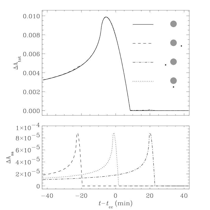
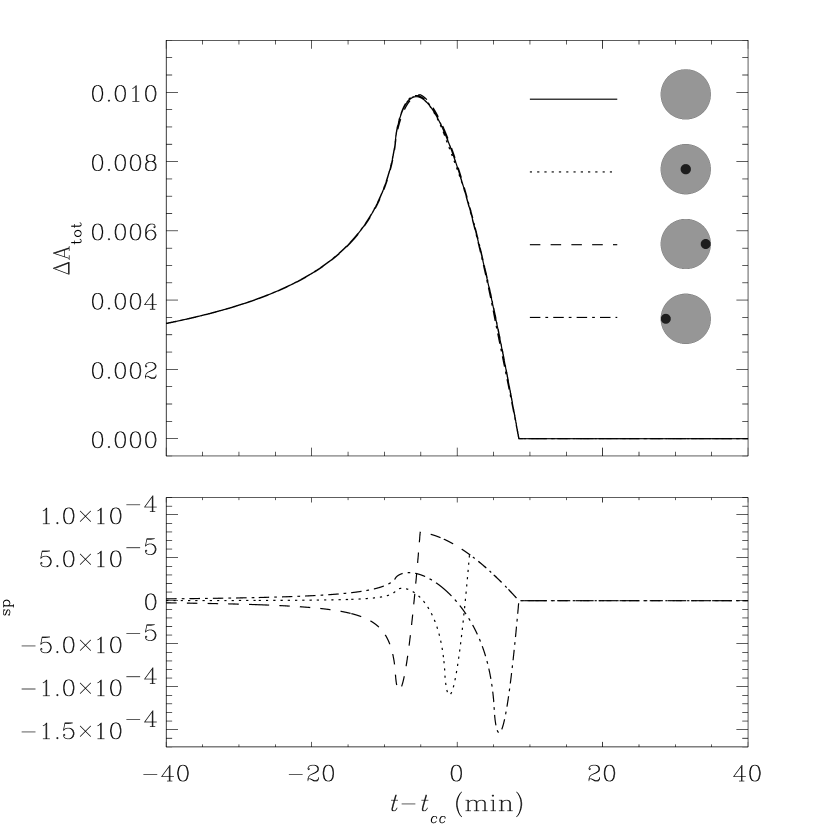
Assuming typical bulge parameters, an analog of the HD209458 system at $D_{\rm os}=8{\rm kpc}$, and for the second caustic crossing of the dashed trajectory in Figure 1, which has the properties $\gamma=71^{\circ}$ and $u_{r}=0.82$, we find $\delta_{\rm p}=7.19\times 10^{-3}$ and $\Delta t_{\rm p}=8.48~{}{\rm min}$. Adopting these parameters, Figure 2 shows the total magnification associated with the planet and satellite, $\Delta A_{tot}=\Delta A_{\rm p}+\Delta A_{\rm sa}$, as well as the extra magnification from the satellite alone, $\Delta A_{\rm sa}$. We show the effect for various satellite positions. The time it takes for the caustic to cross the satellite is $2\Delta t_{\rm sa}\simeq 3.4~{}{\rm min}$.

4.3 Rings

Rings of extrasolar planets have such low mass that they have no observable dynamical effect on the host star’s motion. However, as shown by the example of Saturn’s ring, they can be significantly more extended than planets. This makes them much easier to be identified by transits, for which the signal varies as the area $\Omega$ of the feature that occults the star, and microlensing, for which the signal is $\propto\Omega^{3/4}$ due to the competing effects of the amount of reflected light ($\propto\Omega$), and the magnification ($\propto\Omega^{-1/4}$).

We can obtain an analytic estimate of the signal caused by a ring by assuming a face-on geometry. We model the ring as a circular annulus with uniform surface brightness, outer radius $R_{out}$, and inner radius $R_{in}$. The magnification from the ring is then,

$$\Delta A_{\rm ri}=\delta_{\rm ri}H,$$ (17)

where we have defined

$$H\equiv\left[\left(\frac{R_{out}}{R_{\rm p}}\right)^{3/2}G_{0}(z_{out})-\left(\frac{R_{in}}{R_{\rm p}}\right)^{3/2}G_{0}(z_{in})\right],$$ (18)

and $z_{out}\equiv z_{\rm p}(R_{\rm p}/R_{out})$, and similarly for $z_{in}$. The shape and magnitude of the function $H$ will depend on the relative sizes of $R_{out}$, $R_{in}$, and $R_{\rm p}$, but will generally be of order unity for the ring systems considered here. The magnitude of the deviation due to the ring is therefore roughly $\delta_{\rm ri}$, which in terms of the deviation from the planet is,

$$\delta_{\rm ri}=\kappa_{\rm ri}\delta_{\rm p},$$ (19)

where $\kappa_{\rm ri}={\cal A}_{\rm ri}/{\cal A}_{\rm p}$ is the ratio of the geometric albedos of the ring and planet. We argued in §3 that any surviving ring systems of close-in planets must be rocky in nature, and thus the albedos will generally be small. Adopting $\kappa_{\rm ri}=0.15$, $\delta_{\rm ri}=15\%\delta_{\rm p}$.

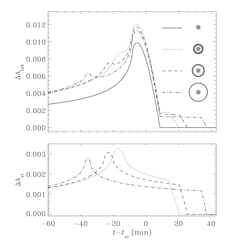
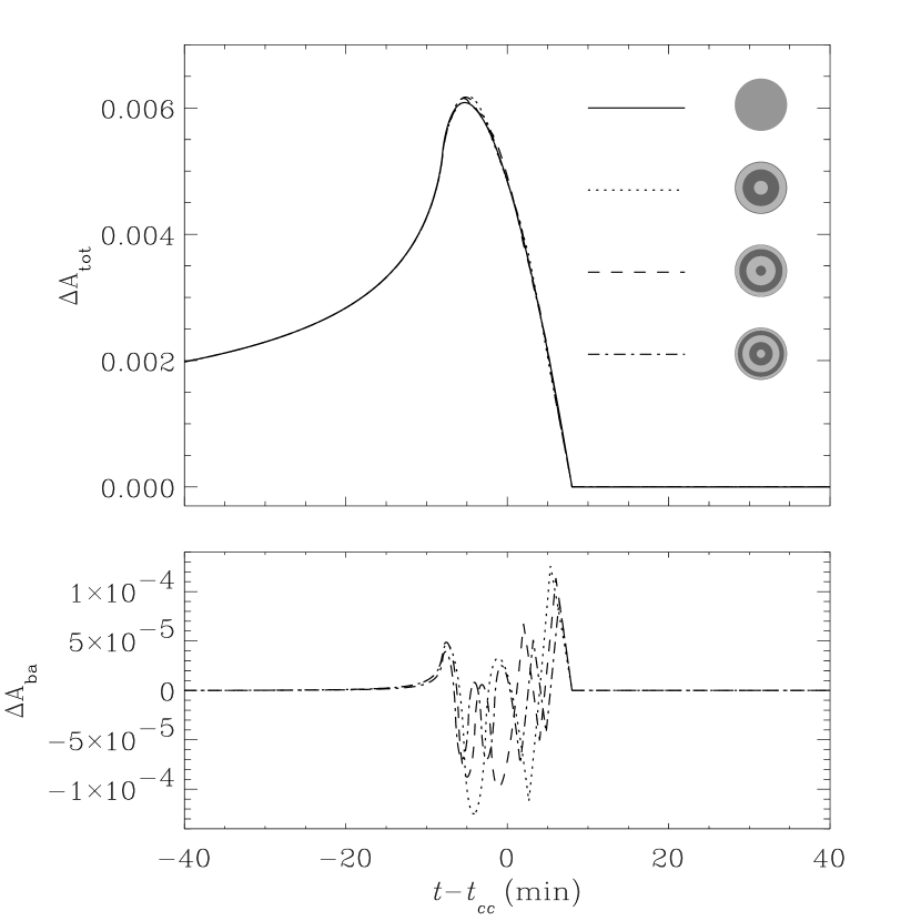
Figure 3 shows the total magnification associated with the planet and ring system, $\Delta A_{tot}=\Delta A_{\rm p}+\Delta A_{\rm ri}$, where we have adopted the same parameters for the planetary deviation as in §4.2, namely $\delta_{\rm p}=7.19\times 10^{-3}$ and $\Delta t_{\rm p}=8.48~{}{\rm min}$. We also show the magnification from the ring system alone, $\Delta A_{\rm ri}$. We show the effect of the ring for various inner radii, and in order to isolate the effect of varying the inner radius on the resulting light curve, we fix the total area of the ring systems to be $\pi(R_{out}^{2}-R_{in}^{2})=10R_{\rm p}^{2}$. The two small bumps on the left and right sides of the primary peak are caused by the ring’s entrance and exit of the caustic. The time between the two ring-induced bumps (or between one of the bumps and the primary peak), relative to the time scale of the planetary perturbation, is a measure of the relative dimension of the ring compared to the size of the planet disk. The time it takes for the caustic to cross the ring system is $2\Delta t_{\rm ri}=2(R_{out}/R_{\rm p})\Delta t_{\rm p}$. For the largest ring system shown in Figure 3, this is $\sim 74~{}{\rm min}$. We find that the signal of the ring generally decreases slowly as the gap between the planet and the ring increases.

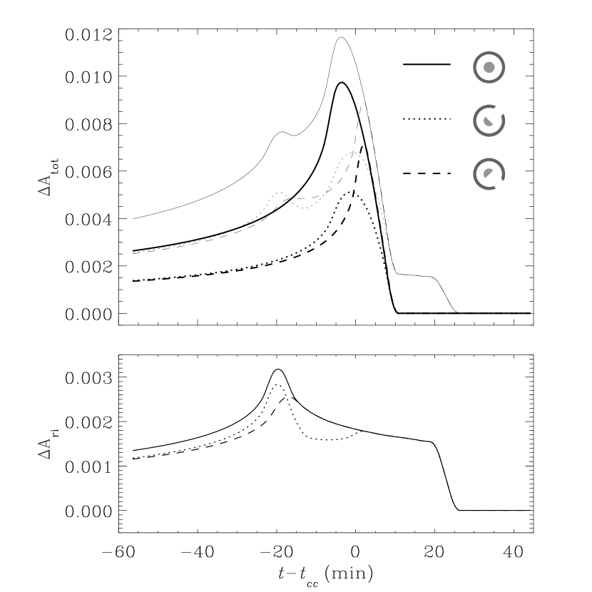
Although our analytical expressions for the deviations induced by a simple, face-on ring system are useful in that they allow one to gain insight and find relatively simply scalings for the magnitude of the effect, they are limited in their scope. In particular, they cannot be used to access the effects of inclined ring systems. For this, numerical integration must be employed in order to calculate the magnification of the ring. We consider sources crossing the second caustic of the dashed trajectory in Figure 1. To calculate the light curve, we first compute the full binary-lens magnification on each area element on the surface of the source and then average the magnifications of the individual elements, weighting by the surface brightness of each element. We again assume typical microlensing parameters, and a source system analogous to HD 209458 at 8 kpc. This yields $\epsilon_{\rm p}=1.26\times 10^{-4}$, and $\rho_{\rm p}t_{\rm E}=8.02~{}{\rm min}$. The effects of $u_{r}$ and $\gamma$ are included implicitly in our numerical integration of the binary-lens magnification for the specific trajectory we have adopted. For the planet-only case, we find our numerical and analytic light curves agree quite well, indicating that our numerical integrations are accurate, the caustic is well-approximated by a simple linear fold, and that we are using the appropriate values of $\gamma$ and $u_{r}$ in our analytic expressions.

In the numerical simulations, we model ringed planets in the same manner as the analytic calculations. We assume that the ring is an infinitely thin annulus without any gap, with inner and outer radii $R_{in}$ and $R_{out}$, respectively. We assume the planet has a uniform albedo of ${\cal A}_{\rm p}=2/3$ for pure Lambert scattering. We assume that the ring has an albedo of ${\cal A}_{\rm ri}=0.1$, and thus $\kappa_{\rm ri}=0.15$, unless otherwise specified. For the simulations, we take the effects of the planet’s phase and the ring’s inclination into consideration. For some specific geometries of the planet, host star, and the observer, the planet will cast a shadow on the ring. We also take this effect into consideration. We then investigate the variations of the pattern of ring-induced anomalies depending on these various factors affecting the shape of the ring.

Defining the projected shape of a ringed planet requires many parameters, such as the inclination of the ring, the phase angle, the radius of the planet disk, and the inner and outer ring radii. As a result of the large number of parameters, it is often difficult to imagine the planet’s shape based on these parameter values. We therefore simply use small icons to characterize the planet and ring shapes instead of specifying all these parameters whenever we present light curves resulting from specific realizations.

Figure 4 shows the effect of the width of the ring on the light curve. All of the systems have a common inner ring radius and gap between the planet disk and the ring, but different outer ring radii. We have also assumed that the ring system is viewed at an angle of $i=75^{\circ}$ with respect to the normal to the ring plane. Not surprisingly, increasing the width of the ring increases the magnitude and duration of the ring-induced perturbation.

Figure 5 shows the dependence of the ring-induced anomaly pattern on the albedo of the ring particles. We test three different albedos of ${\cal A}_{\rm ri}=0.05$, 0.1, and 0.2 (corresponding to $\kappa_{\rm ri}=0.075$, 0.3, and 0.6), and the difference in the greyscale of the rings in the icons represents the variation of the albedo. As expected, the magnitude of the ring signal is proportional to the albedo of ring particles.

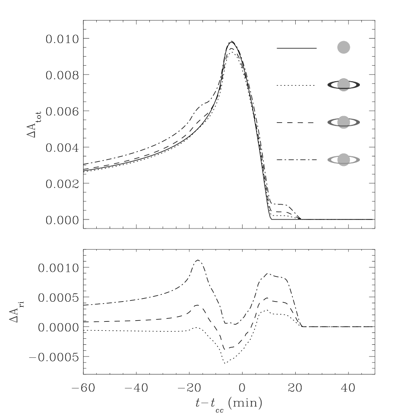
In Figure 6, we demonstrate the effects of a shadow cast on the ring by the planet. In this case, we must also take into account the phase of the planet to be self-consistent. For the geometry depicted in Figure 6, the planet is at quarter phase. We find that the shape of the part of the light curve arising from the planet is strongly dependent on the phase of the planet, as discussed in detail by Ashton & Lewis (2001), however the shape of the signal due the ring does not depend strongly on the effect of the shadow of the planet, due to the relatively small surface area of the ring occulted by the planet.

From the light curves in Figures 4 – 6, we conclude that the typical magnitude of ring-induced deviations is $\delta_{\rm ri}\sim\kappa_{\rm ri}\delta_{\rm p}$, confirming our analytic estimates, although there are considerable variations depending on the inclination and size of the ring.

4.4 Atmospheric Features

In contrast to the signatures of satellites and rings, atmospheric features that are located on the surface of the planet will only produce detectable deviations while the planet is resolved. The planet is only effectively resolved when it is within about one planet radius from the caustic. Therefore, deviations caused by spots, bands, or otherwise non-uniform surface brightness profiles will only be noticeable during a time $\sim 2\Delta t_{\rm p}$ centered on the caustic crossing; outside of this the flux from the planet will essentially be given by the unresolved flux (i.e. the mean surface brightness times the area of the planet disk) times the magnification of a point-source at the center of the planet disk.

4.4.1 Spots

Spots, such as the Great Red Spot on Jupiter, have been observed on the gas giants in our solar system, and are regions of cyclonic activity that have slightly different temperatures and pressures from their surrounding atmospheres. As a result, the colors and albedos of spots are also slightly different. These spots can be quite large relative to the planetary radii; the Great Red Spot has a size larger than $R_{\oplus}$. In this subsection, we provide an analytic estimate of the effect of a spot on the microlensing light curve. We model the spot as a circle of radius $R_{\rm sp}$, with an albedo equal to a fraction $\kappa_{\rm sp}$ of the albedo of the remainder of the planetary surface. The deviation caused by the spot is then,

$$\Delta A_{\rm sp}=\delta_{\rm p}\left\{\frac{1-\kappa_{\rm sp}}{1-(1-\kappa_{\rm sp})\left({R_{\rm sp}}/{R_{\rm p}}\right)^{2}}\left[\left(\frac{R_{\rm sp}}{R_{\rm p}}\right)^{2}G_{0}(z_{\rm p})-\left(\frac{R_{\rm sp}}{R_{\rm p}}\right)^{3/2}G_{0}(z_{\rm sp})\right]\right\}.$$ (20)

Note that, in deriving equation (20), the mean surface brightness of the spotted planet has been normalized to that of the planet without the spot. This ensures that the magnifications of the two cases are identical when the source is not resolved. That this is true can be seen by noting that, for $z_{\rm sp},z_{\rm p}\rightarrow-\infty$, the term in square brackets goes to zero, because $G_{0}(z_{\rm sp})\rightarrow(R_{\rm sp}/R_{\rm p})^{1/2}G_{0}(z_{\rm p})$. Since we are generally concerned with small spots with $R_{\rm sp}/R_{\rm p}\ll 1$, we can make an estimate of the magnitude $\delta_{\rm sp}$ of the deviation caused by the spot by ignoring terms in equation (20) of order $(R_{\rm sp}/R_{\rm p})^{2}$ or higher, and looking at the resulting coefficient to the $G_{0}(z_{\rm sp})$ function. We find that

$$\delta_{\rm sp}\simeq-(1-r_{\rm sp})\left(\frac{R_{\rm sp}}{R_{\rm p}}\right)^{3/2}\delta_{\rm p}.$$ (21)

For $\kappa_{\rm sp}=0.8$, and $R_{\rm sp}=0.2R_{\rm p}$ ($\sim 2R_{\oplus}$ for $R_{\rm p}=R_{Jup}$), we find $\delta_{\rm sp}\simeq 2\%\delta_{\rm p}$.

In Figure 7, we show the total magnification $\Delta A_{tot}$, with and without a spot of radius $R_{\rm sp}=0.2R_{\rm p}$ and relative albedo $\kappa_{\rm sp}=0.8$. We have adopted the same parameters as in §§ 4.2 and 4.3, $\delta_{\rm p}=7.19\times 10^{-3}$ and $\Delta t_{\rm p}=8.48~{}{\rm min}$. We vary the position of the spot as shown. We also show $\Delta A_{\rm sp}$, the deviation caused by the spot from the light curve of a planet with uniform surface brightness. We find the magnitude of the deviation caused by the spot to be $\sim 1\%\delta_{\rm p}$, in rough agreement with our analytic estimate. Since, for linear fold caustics, the magnification is independent of position along the direction parallel to the caustic, the results in Figure 7 are applicable for any circular spot located on the star at the same perpendicular distance from the caustic as the spots shown. Microlensing of spotted planets is analogous to microlensing of spotted stars, see Han et al. (2000), Lewis (2001), and Chang & Han (2002) for examples of such lightcurves.

4.4.2 Zonal Bands

As can be seen on the surface of Jupiter, gaseous giant planets may exhibit color variations on their surface, e.g. zonal bands, which will cause surface brightness variations within a given spectral band. In this subsection, we investigate whether zonal bands can produce noticeable signatures in lensing light curves.

We model zonal bands by stripes which are parallel with the equator of the planet. We assume that the albedos of these stripes alternate with relative values $\kappa_{\rm ba}$, and we vary the total number of stripes. Analytic estimates are generally impossible for arbitrary inclinations of the planet, however, for the special case when the planet is seen pole-in, the pattern of the zonal bands is simply concentric annuli with alternating albedos. In this case, we can find a semi-analytic expression for the deviation from a uniform surface brightness due to the zonal bands. The resulting expression is somewhat complicated,

$$\Delta A_{\rm ba}=\delta_{\rm p}\left[\frac{1-\kappa_{\rm ba}}{1-(1-\kappa_{\rm ba}){(\tilde{R}_{\rm ba}/R_{\rm p})^{2}}}H^{\prime}\right],$$ (22)

where

$$H^{\prime}\equiv\left(\frac{\tilde{R}_{\rm ba}}{R_{\rm p}}\right)^{2}G_{0}(z_{\rm p})-\sum_{i=1}^{N_{\rm ba}-1}(-1)^{i+\ell}\left(\frac{R_{{\rm ba},i}}{R_{\rm p}}\right)^{3/2}G_{0}(z_{{\rm ba},i}),$$ (23)

and $N_{\rm ba}$ is the number of bands, $R_{{\rm ba},i}$ is the outer radius of the $i$th band, $z_{b,i}\equiv z_{\rm p}(R_{\rm p}/R_{{\rm ba},i})$, $\ell=1$ if $N_{\rm ba}$ is odd, and $\ell=0$ if $N_{\rm ba}$ is even, and

$${\tilde{R}_{\rm ba}^{2}}\equiv\sum_{i=1}^{N_{\rm ba}-1}(-1)^{i+\ell}R_{{\rm ba},i}^{2}.$$ (24)

Note that, as $N_{\rm ba}\rightarrow\infty$, $\Delta A_{\rm ba}\rightarrow 0$. The term in square brackets in equation (22) cannot be reduced to a simpler expression, and must be calculated explicitly using the analytic form for the $G_{0}$ function.

In Figure 8, we show the total magnification $\Delta A_{tot}$ of the planet, with and without $N_{\rm ba}$ bands with relative albedos $\kappa_{\rm ba}=0.8$, similar to that of the Jupiter (Pilcher & McCord, 1971). We have adopted the same parameters as in the previous sections, except here we consider the second caustic crossing of the solid trajectory in Figure 1, which has the properties $u_{r}=0.31$ and $\gamma=89^{\circ}$. This yields $\delta_{\rm p}=4.41\times 10^{-3}$ and $\Delta t_{\rm p}=8.02~{}{\rm min}$. We vary the number of bands from $N_{\rm ba}=3-5$, and the bands have equally-spaced radii (and thus cover different surface areas on the source). We also show $\Delta A_{\rm ba}$, the normalized deviation caused by the banded structure from the light curve of a planet with uniform surface brightness. We find the magnitude of the deviation caused by the bands to be

$$\delta_{\rm ba}\sim 30\%(1-\kappa_{\rm ba})N_{\rm ba}^{-\beta}\delta_{\rm p}.$$ (25)

Here the scaling with $\kappa_{\rm ba}$ is only approximate. The scaling with $N_{\rm ba}$ depends on the geometry of the zones; $\beta=1$ for zones with equally-spaced $R_{{\rm ba},i}$ (as shown in Fig. 8), whereas $\beta=1/2$ for equal-area bands. For equal-area zones, the numerical coefficient in equation (25) is also somewhat smaller, $\sim 20\%$.

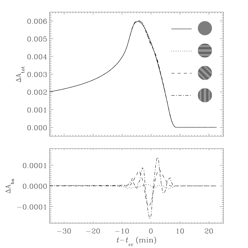
For geometries where the planet is not pole-on, we must resort to numerical calculations. For these calculations, we assume a total of nine bands (with four dark lanes), with relative albedos of $\kappa_{\rm ba}=0.8$, as in the previous example. The albedos are normalized such that the average albedo is $2/3$. Figure 9 shows the effect of zonal bands for a planet with inclination $i=90$ (i.e. the axis of rotation in the plane of the sky), and various orientations of the equator with respect to the caustic. As before, we assume the source trajectory indicated by the solid line in Figure 1. The solid curve is the light curve resulting from a planet having a uniform surface brightness with ${\cal A}_{\rm p}$. From the figure, one finds that the deviations induced by the zonal bands are $\sim 1\%\delta_{\rm p}$, similar to the pole-on case. Note that these deviations are generally an order of magnitude smaller than the typical deviations induced by rings.

4.4.3 Lambert Sphere Scattering

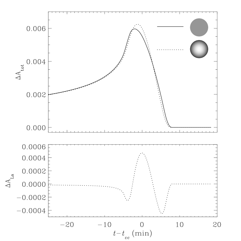
Even without any irregular structure, the surface brightness profile of a planet will generally not be uniform due to projection effects, and the scattering properties of the atmosphere. The surface brightness distribution will therefore vary depending on the latitude $\psi$ and longitude $\omega$ of the planet’s surface as well as the planet’s phase angle, $\alpha$. To illustrate the pattern of lensing light curve deviations caused by a realistic atmosphere, we adopt the simple assumption of pure Lambert scattering, where the incident radiation from the host star is scattered isotropically. Under this assumption, it can be shown that the surface brightness profile is

$$S(\alpha,\omega,\psi)={\bar{S}}\frac{3}{2}\frac{\cos(\alpha-\omega)\cos\omega\cos^{2}{\psi}}{\Phi(\alpha)},\qquad{\bar{S}}=\frac{F_{\rm p}}{\pi\theta_{\rm p}^{2}},$$ (26)

for $\omega\geq\alpha-\pi/2$ and zero otherwise (Sobolev, 1975). Here ${\bar{S}}$ is the mean surface brightness of the planet, and $\Phi(\alpha)$ is the phase integral introduced in §4.1 and displayed explicitly in equation (12). We show the surface brightness distribution for a Lambert sphere with $\alpha=0$ in Figure 10, along with the resulting microlensing light curve. As in §4.4.2, we have assumed the solid source trajectory in Figure 1. We compare this to the light curve resulting from a planet with a uniform surface brightness and an albedo equal to the geometric albedo of the Lambert sphere (i.e. ${\cal A}_{\rm p}=2/3$). We find that the light curve of a Lambert sphere differs from a uniform surface brightness profile by $\sim 10\%\delta_{\rm p}$. The light curve from a Lambert sphere is more highly magnified, due to the fact that the surface brightness profile is more centrally concentrated, and therefore the source is effectively smaller. The precise shape of the light curve from the planet will depend on the scattering properties of the atmosphere, which in turn depend on the constituents of the atmosphere, such as the size of the condensates (Seager & Sasselov, 2000). Therefore resolution of the planetary caustic crossing would provide invaluable information about the physical processes in the planetary atmosphere. This is complementary to the suggestion by Lewis & Ibata (2000) of probing the planetary atmosphere via polizarization monitoring during the planetary caustic crossing.

5 Detectability

In this section, we review the magnitudes of the effects of the features we have considered, and assess their detectability with current and/or future telescopes. Table 5 summarizes our analytic expressions for the magnitudes $\delta_{x}$ of the deviations caused by each structure $x$ that we considered (satellites, rings, spots, and zonal bands), in terms of the magnitude $\delta_{\rm p}$ of the deviation due to only the planet. Also shown is the characteristic timescale $\Delta t_{x}$ of each deviation, relative to the timescale of the planetary caustic crossing $\Delta t_{\rm p}$.

By approximating the perturbations from each structure $x$ as boxcars with amplitudes $\delta_{x}$ and durations $\Delta t_{x}$, we can write down approximate expressions for the ratio of the signal-to-noise $Q_{x}$ for a given perturbation to the signal-to-noise of the planetary pertrubation,

$$\frac{Q_{x}}{Q_{\rm p}}\sim\left|\frac{\delta_{x}}{\delta_{\rm p}}\right|\left(\frac{\Delta t_{x}}{\Delta t_{\rm p}}\right)^{1/2}.$$ (27)

These ratios are displayed in Table 5; they allow one to easily estimate the detectability of the various features in terms of the detectability of the planetary deviation. For example, if one were to require a signal-to-noise ratio of $Q_{\rm p}=20$ for a secure detection of the planet signal, then signal-to-noise of the deviation from a ring with relative albedo $\kappa_{\rm ri}=0.15$ and relative (outer) radius of $R_{\rm ri}/R_{\rm p}=4$ would be $Q_{\rm ri}\simeq 0.15\times\sqrt{4}\times 20=6$. For reasonable parameters, we expect that $Q_{x}/Q_{\rm p}\ll 1$ for satellites, spots, and bands, whereas for rings $Q_{\rm ri}/Q_{\rm p}\sim 30\%$.

We now provide a more accurate estimate of the expected signal-to-noise for the various features. Assume that a microlensing light curve is monitored continuously from $t_{min}$ to $t_{max}$, for a total duration $T$, with a telescope that collects $n_{\nu}$ photons per second per unit flux. The signal-to-noise ratio $Q_{x}$ of a deviation $\Delta A_{x}(t)$ is then,

$$Q_{x}=(n_{\nu}T)^{1/2}{F_{*}\over(B+F_{*})^{1/2}}\left\{{1\over T}\int_{t_{min}}^{t_{max}}dt\ [\Delta A_{x}(t)]^{2}\right\}^{1/2},$$ (28)

where $F_{*}$ is the unlensed flux of the primary star, and $B$ is the background flux (sky + unresolved stars). The term in curly brackets is essentially the RMS of the deviation during the time of the observations. We assume that the source system is an analog of HD20458 at $D_{\rm os}=8$ kpc. The primary has $I_{*}=19.5$ (a G0V star at $8$ kpc with 1.2 magnitudes of extinction), and its planet has $R_{\rm p}=1.347R_{Jup}$, $a=0.0468~{}{\rm AU}$, and ${\cal A}_{\rm p}=2/3$. Adopting typical bulge parameters ($M=0.3M_{\odot},D_{\rm ol}=6~{}{\rm kpc},D_{\rm os}=8~{}{\rm kpc}$), and a caustic crossing with properties $u_{r}=1$ and $\gamma=90^{\circ}$, this gives $\delta_{\rm p}=7.93\times 10^{-3}$ and $\Delta t_{\rm p}=8~{}{\rm min}$. We assume a total background flux of $19.3$, which includes the moon-averaged sky background at an average site, and the contribution expected from unresolved stars in the bulge for a seeing of $0.75^{\prime\prime}$. We assume that a telescope of diameter $A_{T}$ collects $n_{\nu}=2700(A_{T}/10~{}{\rm m})^{2}$ photons per second at $I=20$, which corresponds to an overall throughput (including detector efficiency) of $\sim 50\%$. Finally, we assume that the light curve is monitored from $-5\Delta t_{\rm p}$ before the caustic crossing until $5\Delta t_{\rm p}$ after the caustic crossing of the primary star, for a total duration of $T\simeq 80~{}$min.

The resulting signal-to-noise values for the various deviations are tabulated in Table 5. For 10m-class telescopes, the deviation from the planet should be detectable with $Q_{\rm p}\simeq 15$. This is in rough agreement with the results of Graff & Gaudi (2000) and Ashton & Lewis (2001) for full phases. However, Ashton & Lewis (2001) find that the signal-to-noise depends quite strongly on the phase of the planet. Adopting a different phase would therefore affect the relative signal-to-noise $Q_{x}/Q_{\rm p}$ between the planet and the satellite, ring, spot or band features, but generally not the absolute signal-to-noise $Q_{x}$. For the deviations from the other structures, we have adopted the parameter values appropriate to the short-dashed line in Figure 2 for the satellite, the dotted line in Figure 3 for the ring, the short-dashed line in Figure 7 for the spot, and the long-dashed line in Figure 8 for the zonal bands. For these perturbations we find signal-to-noise ratios of $Q_{\rm sa}=0.1$ (satellite), $Q_{\rm ri}=6.1$ (ring), $Q_{\rm sp}=0.1$ (spot), and $Q_{\rm ba}=0.1$ (zonal bands). These are in rough agreement with the expected scaling with $Q_{\rm p}$, and generally indicate that it will be impossible to detect spots, bands, and satellites with 10m-class telescopes. Rings are potentially detectable, but only under somewhat optimistic scenarios, i.e. large, face-on rings. We therefore consider the detectability with larger-aperture telescopes, such as the proposed 30-meter aperture California Extremely Large Telescope (CELT) (Nelson, 2000), or the European Space Agency’s proposed 100-meter aperture Overwhelmingly Large Telescope (OWL) (Dierickx & Gilmozzi, 2000). We find that rings will generally be detectable with reasonable signal-to-noise for $A_{T}\gtrsim 30~{}$m, and spots, satellites and bands are likely to be undetectable with any foreseeable telescope.

For the deviations caused by Lambert scattering shown in Figure 10, we find that $Q\sim 1\%Q_{\rm p}$. Therefore, the non-uniform nature of the surface brightness may be measurable with 100m-class telescopes.

Feature	Magnitude	Timescale	Relative $S/N$	Absolute $S/N$
	$\delta_{x}/\delta_{\rm p}$	$\Delta t_{x}/\Delta t_{\rm p}$	$Q_{x}/Q_{\rm p}$	10m	30m	50m	100m
Planet	$\delta_{\rm p}=\epsilon_{\rm p}\left({u_{r}\over\rho_{\rm p}}\right)^{1/2}$	–	–	15.1	45.2	75.4	150.7
Satellite	$\kappa_{\rm sa}\left(\frac{R_{\rm sa}}{R_{\rm p}}\right)^{3/2}$	$\frac{R_{\rm sa}}{R_{\rm p}}$	$\kappa_{\rm sa}\left(\frac{R_{\rm sa}}{R_{\rm p}}\right)^{2}$	0.1	0.2	0.3	0.7
Ring	$\kappa_{\rm ri}$	$\frac{R_{\rm ri}}{R_{\rm p}}$	$\kappa_{\rm ri}\left(\frac{R_{\rm ri}}{R_{\rm p}}\right)^{1/2}$	6.1	18.4	30.7	61.4
Spot	$-(1-\kappa_{\rm sp})\left(\frac{R_{\rm sp}}{R_{\rm p}}\right)^{3/2}$	$\frac{R_{\rm sp}}{R_{\rm p}}$	$(1-\kappa_{\rm sp})\left(\frac{R_{\rm sp}}{R_{\rm p}}\right)^{2}$	0.1	0.3	0.5	0.9
Bands	$0.3(1-\kappa_{\rm ba})N_{\rm ba}^{-\beta}$	1	$0.3(1-\kappa_{\rm ba})N_{\rm ba}^{-\beta}$	0.1	0.3	0.6	1.1

Table 1 Estimated Signal-to-Noise Ratios for Planetary Structures.

6 Summary and Conclusion

Planetary companions to the source stars of caustic crossing microlensing events can be detected via the brief deviation created when the caustic transits the planet, magnifying the reflected light from the star. The magnitude of the planetary deviation is $\delta_{\rm p}\sim\epsilon_{\rm p}\rho_{\rm p}^{-1/2}$, where $\epsilon_{\rm p}$ is the fraction of the flux of the star that is reflected by the planet, and $\rho_{\rm p}$ is the angular size of the planet in units of the angular Einstein ring radius of the lens. For giant, close-in planets (similar to HD20958b), $\epsilon_{\rm p}\sim 10^{-4}$, and for typical events toward the Galactic bulge, $\rho_{\rm p}\sim 10^{-4}$. Thus $\delta_{\rm p}\sim 1\%$, which is accessible to 10m-class ground-based telescopes.

Due to the extraordinarily high angular resolution afforded by caustic crossings, fine structures in and around the planet are, in principle, also detectable. We first presented a brief discussion on the existence and stability of satellites, rings and atmospheric features of close-in planets, concluding that although rings and satellites may be short-lived due to dynamical forces, the ultimate fate of such structures is not clear. There are good reasons to believe that atmospheric features may be important in close-in planets. We therefore considered the signatures of satellites, rings, spots, zonal bands, and non-uniform surface brightness profiles on the light curves of planetary caustic-crossings. Where possible, we used semi-analytic approximations to derive useful expressions for the magnitude of the deviations expected for these features, as a function of the relevant parameters, such as the albedo or size of the feature. We express these deviations in terms of $\delta_{\rm p}$, the magnitude of the planetary deviation.

We find that rings produce deviations of amplitude $\sim 10\%\delta_{\rm p}$, whereas spots, zonal bands, and satellites all produce deviations of order $\sim 1\%\delta_{\rm p}$. These semi-analytic estimates are supported by more detailed numerical simulations. We also find that the light curve of a planet with the surface brightness profile expected from Lambert scattering deviates from that of a uniform source by $\sim 10\%\delta_{\rm p}$. This affords the possibility of probing the physical processes of the atmospheres of distant extrasolar planets by constraining their surface brightness profiles, and therefore the scattering properties of their constituent particles.

We assessed the detectability of spots, rings, satellites, and bands with current and future telescopes. We found that, for reasonable assumptions and 10m-class telescopes, the planetary deviation will have a signal-to-noise of $\sim 15$, a ring system will only be marginally detectable with a signal-to-noise of $\sim 6$, and all other features will be completely undetectable. For 30m-class or larger telescopes, rings should be easily detectable, The detection of the non-uniform nature of the planetary surface brightness profile arising from Lambert scattering requires 100m-class telescopes for bare detection. Spots, satellites and zonal bands are essentially undetectable for even the largest telescopes apertures.

Figure 1: An example of the caustic structure (thick solid curve) produced by a binary lens. In this case, the system has equal mass components separated by one Einstein ring radius. The coordinates are centered at the midpoint of the binary, and all lengths are normalized by the Einstein ring radius. The solid and dashed straight lines are the two source trajectories considered in the numerical simulations. The insets are the details of the regions around the second caustic crossings of these trajectories.

Figure 2: Top: Caustic-crossing microlensing light curves from a planet with and without a satellite with radius equal to 20% of the radius of the planet, and albedo equal to 10% of the planet’s albedo. The solid line shows the light curve from the planet only. The other lines show the magnification including a satellite with various relative positions. The events arise from the second caustic crossing of the dashed source trajectory through the binary-lens systems depicted in Fig. 1. Bottom: The additional magnification $\Delta A_{\rm sa}$ caused by the satellite alone.

Figure 3: Top: Caustic-crossing microlensing light curves from a planet with and without a face-on ring with different gaps between the planet’s disk and the ring. The solid line shows the light curve from the planet only. The icons show the ring geometries for the corresponding light curves with rings. The inner ring radius is $R_{\rm ri}=1.6$ (dotted), 2.4 (short-dashed), and $4.0R_{\rm p}$ (long-dashed), respectively, where $R_{\rm p}$ is the radius of the planet. The outer ring radius is adjusted so that the projected area of the ring is equal to $\pi(R_{out}^{2}-R_{in}^{2})=10R_{\rm p}^{2}$. The ring has an albedo equal to 15% of the albedo of the planet. The lens system and the source trajectory responsible for the events are the same as for the light curves presented in Fig. 2. Bottom: The additional magnification $\Delta A_{\rm ri}$ caused by the ring alone.

Figure 4: Top: Caustic-crossing microlensing light curves from a planet with inclined rings of different widths. The rings have a common inner radius of $R_{in}=2.0\ R_{\rm p}$, but different outer ring radii of $R_{out}=2.6$, 3.0, and 4.0 $R_{\rm p}$. The ring has an inclination of $i=75^{\circ}$, and albedo relative to the planet of $15\%$. The lens system and the source trajectory responsible for the events are the same as for the light curves presented in Fig. 2. Bottom: The additional magnification $\Delta A_{\rm ri}$ caused by the ring alone.

Figure 5: Top: Caustic-crossing microlensing light curves from a planet with inclined rings with different albedos. The total magnification is shown for a planet with rings of equal size, [inner and outer ring radii of $(R_{in},R_{out})=(2.0,2.6)R_{\rm p}$], but relative albedos of $\kappa_{\rm ri}=0.075$ (solid), 0.3 (dotted), and 0.6 (dashed). The inclination of the rings is $i=75^{\circ}$. The lens system and the source trajectory responsible for the events are the same as for the light curves presented in Fig. 2. Bottom: The additional magnification $\Delta A_{\rm ri}$ caused by the ring alone.

Figure 6: Top: Caustic-crossing microlensing light curves from a planet with a ring, where the planet’s shadow is cast on the ring. Note that, due to the specific geometry of the planet, host star, and observer, the planet is at quarter phase. Each ring has inner and outer ring radii of $(R_{in},R_{out})=(2.4,3.0)R_{\rm p}$, is seen face-on, and has an albedo relative to the planet of 15%. The lens system and the source trajectory responsible for the events are the same as for the light curves presented in Fig. 2. For all line types, the heavier curve is for the planet only, while the lighter curve is for the planet and the ring. Bottom: The additional magnification $\Delta A_{\rm ri}$ caused by the ring alone.

Figure 7: Top: Caustic-crossing microlensing light curves from a planet with and without a spot with radius equal to 20% of the radius of the planet, and albedo equal to 80% of the planet’s albedo. The solid line shows the light curve from the planet only, the magnitude of the deviation due to the planet. The other lines show the magnifications including a spot with various relative positions. The lens system and the source trajectory responsible for the events are the same as for the light curves presented in Fig. 2. Bottom: The deviation $\Delta A_{\rm sp}$ due to the spot.

Figure 8: Top: Caustic-crossing microlensing light curves from a planet with and without surface albedo variations caused by zonal bands. The zonal bands are parallel with the planet’s equator and cause alternate variations of the surface brightness, and the planet is seen pole-on. The albedos of the bright and dark regions differ by $20\%$, and the mean surface brightness of each model has been adjusted in order to match that from the uniform planet. The events arise from the second caustic crossing of the solid source trajectory through the binary-lens systems depicted in Fig. 1. Bottom: The deviation $\Delta A_{\rm ba}$ caused by the zonal bands.

Figure 9: Top: Caustic-crossing microlensing light curves from a planet with and without zonal bands. The zonal bands are parallel with the planet’s equator and cause alternate variations of the surface brightness, and the inclination of the planet is $90^{\circ}$. The albedos of the bright and dark regions differ by $20\%$. The solid curve is the lensing light curve corresponding to a planet with uniform surface brightness. The lens system and the source trajectory responsible for the events are the same as for the light curves presented in Fig. 8. Bottom: The deviation $\Delta A_{\rm ba}$ caused by the zonal bands.

Figure 10: Top: Caustic-crossing microlensing lensing light curves from a planet with the surface brightness profile expected from Lambert scattering (dotted), and a uniform surface brightness profile (solid). The lens system and the source trajectory responsible for the events are the same as for the light curves presented in Fig. 8. Bottom: The deviation $\Delta A_{\rm La}$ in the magnification of a Lambert sphere from a source with uniform surface brightness.

References

- Afonso et al. (2000) Afonso, C., et al. 2000, ApJ, 532, 340
- Albrow et al. (1999) Albrow, M. D. et al. 1999, ApJ, 522, 1011
- Albrow et al. (2001) Albrow, M. et al. 2001a, ApJ, 549, 759
- Albrow et al. (2001) Albrow, M. et al. 2001b, ApJ, 550, L173
- Alcock et al. (2000) Alcock, C., et al. 2000, ApJ, 541, 270
- An et al. (2002) An, J. H. et al. 2002, ApJ, 572, 521
- Ashton & Lewis (2001) Ashton, C. E., & Lewis, G. F. 2001, MNRAS, 325, 305
- Barnes & O’Brien (2002) Barnes, J. W., & O’Brien, D. P. 2002, ApJ, 575, 1087
- Bennett & Rhie (1996) Bennett, D. P., & Rhie, S. H. 1996, ApJ, 472, 660
- Brown et al. (2001) Brown, T. M., Charbonneau, D., Gilliland, R. L., Noyes, R. W., & Burrows, A. 2001, ApJ, 552, 699
- Brown, Libbrecht, & Charbonneau (2002) Brown, T. M., Libbrecht, K. G., & Charbonneau, D. 2002, PASP, 114, 826
- Burrows et al. (1997) Burrows, A. et al. 1997, ApJ, 491, 856
- Burrows et al. (2000) Burrows, A., Guillot, T., Hubbard, W. B., Marley, M. S., Saumon, D., Lunine, J. I., & Sudarsky, D. 2000, ApJ, 534, L97
- Castro et al. (2001) Castro, S., Pogge, R. W., Rich, R. M., DePoy, D. L., & Gould, A. 2001, ApJ, 548, L197
- Chang (1984) Chang, K. 1984, A&A, 130, 157
- Chang & Han (2002) Chang, H.-Y., & Han, C. 2002, MNRAS, 335, 195
- Charbonneau et al (2000) Charbonneau, D., Brown, T. M., Latham, D. W., & Mayor, M. 2000, ApJ, 529, L45
- Charbonneau et al. (2002) Charbonneau, D., Brown, T. M., Noyes, R. W., & Gilliland, R. L. 2002, ApJ, 568, 377
- Cho et al. (2003) Cho, J. Y.-K., Menou, K., Hansen, B., & Seager, S. 2002, ApJ, submitted (astro-ph/0209227)
- Cochran et al. (1997) Cochran, W. D., et al. 1997, ApJ, 483, 457
- Dierickx & Gilmozzi (2000) Dierickx, P., & Gilmozzi, R. 2000, Proc. SPIE, 4004, 290
- Erdl & Schneider (1993) Erdl, H., & Schneider, P. 1993, A&A, 268, 453
- Fortney et al. (2003) Fortney, J. J., et al. 2002, ApJ, submitted (astro-ph/0208263)
- Gaudi & Petters (2002) Gaudi, B. S. & Petters, A. O. 2002, ApJ, 574, 970
- Gaudi (2003) Gaudi, B.S. 2003, in ASP Conf. Ser. 000: Scientific Frontiers in Research on Extrasolar Planets, eds. D. Deming and S. Seager (ASP: San Francisco), 000 (astro-ph/0207533)
- Goldreich & Tremaine (1982) Goldreich, P. & Tremaine, S. 1982, ARA&A, 20, 249
- Gonzalez (1997) Gonzalez, G. 1997, MNRAS, 285, 403
- Gonzalez (1998) Gonzalez, G. 1998, A&A, 334, 221
- Goukenleuque et al. (2000) Goukenleuque, C., Bézard, B., Joguet, B., Lellouch, E., & Freedman, R. 2000, Icarus, 143, 308
- Gould & Loeb (1992) Gould, A., & Loeb, A. 1992, ApJ, 396, 104
- Graff & Gaudi (2000) Graff, D. S., & Gaudi, B. S. 2000, ApJ, 538, L133
- Guillot & Showman (2002) Guillot, T. & Showman, A. P. 2002, A&A, 385, 156
- Han et al. (2000) Han, C., Park, S.-H., Kim, H.-I., & Chang, K. 2000, MNRAS, 316, 665
- Henry et al. (2000) Henry, G. W., Marcy, G. W., Butler, R. P., & Vogt, S. S. 2000, ApJ, 529, L41
- Hui & Seager (2002) Hui, L. & Seager, S. 2002, ApJ, 572, 540
- Heyrovský & Sasselov (2000) Heyrovský, D. & Sasselov, D. 2000, ApJ, 529, 69
- Jaroszyński (2002) Jaroszyński, M. 2002, preprint (astro-ph/0203476)
- Jaroszynski & Paczynski (1995) Jaroszynski, M. & Paczynski, B. 1995, ApJ, 455, 443
- Karkoschka (1994) Karkoschka, E. 1994, Icarus, 111, 174
- Laughlin (2000) Laughlin, G. 2000, ApJ, 545, 1064
- Lee, Chang, & Kim (1998) Lee, D. W., Chang, K. A., & Kim, S. J. 1998, JKAS, 31, 27
- Lewis (2001) Lewis, G. F. 2001, A&A, 380, 292
- Lewis & Ibata (2000) Lewis, G. F., & Ibata, R. A. 2000, ApJ, 539, L63
- Mao & Paczyński (1991) Mao S., & Paczyński B. 1991, ApJ, 374, L37
- Marcy & Butler (1998) Marcy, G., & Butler, R. 1998, ARA&A, 36, 57
- Marcy & Butler (2000) Marcy, G., & Butler, R. 1998, PASP, 112, 137
- Mayor & Queloz (1995) Mayor, M., & Queloz, D. 1995, Nature, 378, 355
- Nelson (2000) Nelson, J. E. 2000, Proc. SPIE, 4004, 282
- Noyes et al. (1997) Noyes, R. W., et al. 1997, ApJ, 483, L111
- Pätzold & Rauer (2002) Pätzold, M. & Rauer, H. 2002, ApJ, 568, L117
- Perryman (2000) Perryman, M. A. C. 2000, Rep. Prog. Phys., 63, 1209
- Pilcher & McCord (1971) Pilcher, C. B., & McCord, T. B. 1971, ApJ, 165, 195
- Reid (2002) Reid, I. N. 2002, PASP, 114, 306
- Santos, Israelian, & Mayor (2001) Santos, N. C., Israelian, G., & Mayor, M. 2001, A&A, 373, 1019
- Sartoretti & Schneider (1999) Sartoretti, P. & Schneider, J. 1999, A&AS, 134, 553
- Saumon et al. (1996) Saumon, D., Hubbard, W. B., Burrows, A., Guillot, T., Lunine, J. I., & Chabrier, G. 1996, ApJ, 460, 993
- Schneider (1999) Schneider, J. 1999, CR Acad. Scie. Ser. II, 327, 621
- Schneider, Ehlers & Falco (1992) Schneider, P., Ehlers, J., & Falco, E. E. 1992, Gravitational Lenses (Berlin: Springer)
- Schneider & Weiss (1986) Schneider, P., & Weiss, A. 1986, A&A, 164, 237
- Schneider & Weiss (1986) Schneider, P. & Weiss, A. 1987, A&A, 171, 49
- Seager & Hui (2002) Seager, S. & Hui, L. 2002, ApJ, 574, 1004
- Seager & Sasselov (1998) Seager, S. & Sasselov, D. D. 1998, ApJ, 502, L157
- Seager & Sasselov (2000) Seager, S. & Sasselov, D. D. 2000, ApJ, 537, 916
- Seager, Whitney, & Sasselov (2000) Seager, S., Whitney, B. A., & Sasselov, D. D. 2000, ApJ, 540, 504
- Showman & Guillot (2002) Showman, A. P. & Guillot, T. 2002, A&A, 385, 166
- Sobolev (1975) Sobolov, V. V. 1975, Light Scattering in Planetary Atmospheres (Oxford: Pergamon)
- Ulmer & Goodman (1995) Ulmer, A. & Goodman, J. 1995, ApJ, 442, 67
- Ward & Reid (1973) Ward, W. R. & Reid, M. J. 1973, MNRAS, 164, 21
- Wolszcan & Frail (1992) Wolszczan, A., & Frail, D. A. 1992, Nature, 355, 145
- Zucker & Mazeh (2002) Zucker, S. & Mazeh, T. 2002, ApJ, 568, L113