Galactic Synchrotron Foreground and the CMB Polarization Measurements

Abstract

The polarization of the Cosmic Microwave Background (CMB)is a powerful observational tool at hand for modern cosmology. It allows to break the degeneracy of fundamental cosmological parameters one cannot obtain using only anisotropy data and provides new insight into conditions existing in the very early Universe. Many experiments are now in progress whose aim is detecting anisotropy and polarization of the CMB. Measurements of the CMB polarization are however hampered by the presence of polarized foregrounds, above all the synchrotron emission of our Galaxy, whose importance increases as frequency decreases and dominates the polarized diffuse radiation at frequencies below $\simeq 50$ GHz. In the past the separation of CMB and synchrotron was made combining observations of the same area of sky made at different frequencies. In this paper we show that the statistical properties of the polarized components of the synchrotron and dust foregrounds are different from the statistical properties of the polarized component of the CMB, therefore one can build a statistical estimator which allows to extract the polarized component of the CMB from single frequency data also when the polarized CMB signal is just a fraction of the total polarized signal. This estimator improves the signal/noise ratio for the polarized component of the CMB and reduces from $\simeq$50 GHz to $\simeq$20 GHz the frequency above which the polarized component of the CMB can be extracted from single frequency maps of the diffuse radiation.

1 Introduction

This year is a decade since the first detection of the anisotropy of the Cosmic Microwave Background at large angular scales ($\geq 10^{0}$) [1], [2]. Today the CMB anisotropy (CMBA) has been detected also at intermediate ($\sim(1^{0}-10^{0})$) and small angular scales ($\leq 1^{0}$), so the CMBA angular spectrum is now reasonably known down to the region of the first and second Doppler peaks [3], [4], [5]. Its shape gives information e.g. on the spectrum of the primordial cosmological perturbations or can be used to test the inflation theory but rises new questions to which CMBA cannot answers. Responses can on the contrary be obtained looking at the CMB polarization (CMBP) produced by Thomson scattering of CMB photons on the matter anisotropies at the recombination epoch. In particular one can hope to use CMBP to disentangle the effects of fundamental cosmological parameters like density of matter, density of dark energy etc., effects anisotropy do not separate.This is among the goals of space and ground based experiments like [6], [7], [8], [9], [10], [11], [12] and is the main goal of SPOrt a polarization dedicated ASI/ESA space mission on the International Space Station [13]. The relevance of the CMB polarization was remarked for the first time by M. Rees [14]. Since him many models of the expected features of the CMBP have been published (see for instance [15], [16], [17]). They stimulated the search for CMBP, but in spite of many attempts so far no CMB polarization has been detected. This observation is in fact extremely difficult because the expected signal is at least an order of magnitude smaller than the amplitude of the CMBA. Moreover foregrounds and their inhomogeneities cover the polarized fraction of the CMB or mimic CMBP spots, making the signal to noise (CMBP $/$ polarized foreground) ratio unfavorable. In this paper we will concentrate on methods for improving this ratio and for disentangling CMBP and polarized foregrounds.

In the microwave range the galactic foregrounds include:

• synchrotron radiation (strongly polarized),

• free-free emission (polarization negligible),

• dust radiation.

Because here we are interested in polarization, in the following we will neglect the free-free emission, whose expected level of polarization is negligible. Moreover the polarized signals produced by dust, if present, (e.g. [18], [19]), may be treated as an addition to the synchrotron effects. In fact, as it will appears in the following, the important quantities in our analysis are the statistical properties of the foreground spatial distribution and, by good fortune, the spatial distribution of the dust polarized emission is similar to that of the synchrotron emission, since behind both radiation types there is the same driving force, the galactic magnetic field which alignes dust grains and guides radiating electrons.

Separation of foregrounds and CMBA was successfully solved when the CMB anisotropy was discovered [2]. When we go from CMBA to CMBP the separation of foreground and background however is more demanding and the problem of discriminating foreground inhomogneities from true CMB spots severe. Approaches used in the past e.g. [20], [21], [22], [23], [24]) were essentially based on the differences between the frequency spectra of foregrounds and CMB, therefore require multifrequency observations.

In this paper we suggest a different method which takes advantage of the fact that the measured values of the parameters we use to describes the polarization of the diffuse radiation when measured at a given frequency in different directions behave as stochastic variables. Because the mathematical and statistical properties of these variables for synchrotron and CMB are different, we suggest to use statistical methods for analyzing single frequency maps of the diffuse radiation and disentangling their main components, synchrotron and CMBP. This method was proposed and briefly discussed in [25]. Here we present a more complete analysis.

2 Polarization Parameters

2.1 The Stokes Parameters

Convenient quantities commonly used to describe the polarization status of radiation are the Stokes parameters (see for instance [26], [27], [28]). Let’s assume a monochromatic, plane, wave of intensity I and amplitude $\propto\sqrt{I}$. In the observer plane, orthogonal to the direction of propagation of the electromagnetic wave emitted by the electron, we can choose a pair of orthogonal axes ${\vec{l}}$ and ${\vec{r}}$. On that plane the amplitude vector of an unpolarized wave moves in a random way. On the contrary it describes a figure, the polarization ellipse, when the wave is polarized.

Projecting the wave amplitude on ${\vec{l}}$ and ${\vec{r}}$ we get two orthogonal, linearly polarized, waves of intensity $I_{l}$ and $I_{r}$,($I=I_{l}+I_{r}$) whose amplitudes are $\propto\sqrt{I_{l}}$ and $\propto\sqrt{I_{r}}$ respectively. If the original wave of intensity $I$ is polarized, $I_{l}$ and $I_{r}$ are correlated: let‘s call $I_{12}$ and $I_{21}$ their correlation products.

By definition the Stokes parameters are the four quantities: $I=I_{l}+I_{r}$, $Q=I_{l}-I_{r}$, $U=I_{12}+I_{21}$, and $V=i(I_{21}-I_{12})$.

$Q$ and $U$ describe the linear polarization, $V$ the circular polarization and $I$ the total intensity.

The ratio

$$\tan 2\chi={\displaystyle U\over\displaystyle Q}$$ (1)

gives the angle $\chi$ between the vector $\vec{l}$ and the main axis of the polarization ellipse ($0<\chi<\pi$).

Rotating the $(l,r)$ coordinate system by an angle $\phi$ we get a new coordinate system $(\hat{l},\hat{r})$ in which the Stokes parameters become

$$\begin{array}[]{c}\hat{Q}=Q\cos 2\phi-U\sin 2\phi\\ {}\hfil\\ \hat{U}=U\cos 2\phi+Q\sin 2\phi\end{array}$$ (2)

When $\phi=\chi=(1/2)\arctan{{\displaystyle U\over\displaystyle Q}}$ the axes of the polarization ellipse coincide with the reference axes $\hat{l}$ and $\hat{r}$ (see fig.1).

         

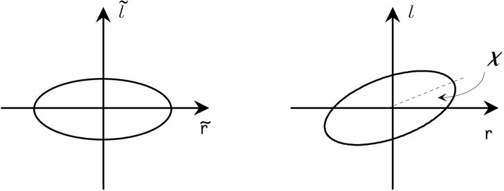
Figure 1: The polarization ellipse

2.2 Electric and Magnetic Modes

To analyze the properties of the CMB polarization it is sometimes convenient to use rotationally invariant quantities, like the radiation intensity $I$ and two combinations of $U$ and $Q$: $Q+iU$ and $Q-iU$. The intensity $I$ can be decomposed into usual (scalar) spherical harmonics $Y_{lm}(\theta,\varphi)$.

$$I=\sum_{l,m}a_{lm}Y_{lm}(\theta,\varphi)$$ (3)

The quantities $Q\pm iU$ can be decomposed into $\pm 2$ spin harmonics [29], [30], [31] $Y_{lm}^{\pm 2}(\theta,\varphi)$ :

$$Q\pm iU=\sum_{l,m}a_{lm}^{\pm 2}Y_{lm}^{\pm 2}(\theta,\varphi)$$ (4)

The $\pm 2$ spin harmonics form a complete orthonormal system (see, for instance, [32],[33], [34], [35]) and can be written [30], [36]:

$$\begin{array}[]{c}Y^{2}_{lm}(\theta,\varphi)=N^{2}_{lm}P^{2}_{lm}(\theta)e^{im\varphi}\\ {}\hfil\\ Y^{-2}_{lm}(\theta,\varphi)=N^{-2}_{lm}P^{-2}_{lm}(\theta)e^{im\varphi}\end{array}$$ (5)

where

$$P^{s}_{lm}(x)=(1-x)^{\displaystyle(m+s)\over 2}(1+x)^{\displaystyle(s-m)\over 2}P^{(m+s,s-m)}_{l-s}(x)$$ (6)

is a generalized Jacobi polynomial, $s=\pm 2$ and:

$$N^{s}_{lm}=\frac{1}{2^{s}}\sqrt{\frac{2l+1}{4\pi}}\sqrt{\frac{(l-s)!(l+s)!}{(l-m)!(l+m)!}}$$

is a normalization factor.

The harmonics amplitudes $a^{\pm 2}_{lm}$ correspond to the Fourier spectrum of the angular decomposition of rotationally invariant combinations of Stokes parameters.

Because spin $\pm 2$ spherical functions form a complete orthonormal system:

$$\int_{4\pi}Y^{\pm 2}_{lm}(\theta,\varphi)Y^{*\;\pm 2}_{l^{\prime}m^{\prime}}(\theta,\varphi)d\Omega=\delta_{lm}\delta_{l^{\prime}m^{\prime}}$$ (7)

we can write

$$a^{\pm 2}_{lm}=\int_{4\pi}d\Omega\;\;\left(Q(\theta,\varphi)\pm iU(\theta,\varphi)\right)Y^{*\;\pm 2}_{lm}$$ (8)

Following [31] we now introduce the so called $E$ (electric) and $B$ (magnetic) modes of these harmonic quantities:

$$\begin{array}[]{c}a^{E}_{lm}=\frac{1}{2}\left(a^{+2}_{lm}+a^{-2}_{lm}\right)\\ {}\hfil\\ a^{B}_{lm}=\frac{i}{2}\left(a^{+2}_{lm}-a^{-2}_{lm}\right)\end{array}$$ (9)

They have different parities. In fact when we transform the coordinate system $Oxyz$ into a new coordinate system $\tilde{O}\tilde{x}\tilde{y}\tilde{z}$, such that

$$\begin{array}[]{c}\tilde{\vec{l}}=\vec{l}\\ \tilde{\vec{r}}=-\vec{r}\end{array}$$ (10)

the E and B modes transform in a similar way:

$$\begin{array}[]{c}\tilde{a}^{E}=a^{E}\\ \tilde{a}^{B}=-a^{B}\end{array}$$ (11)

$Q$ remains identical in both reference systems and $U$ changes sign.

It is important to remark that $a^{E}$ and $a^{B}$ are uncorrelated.

In terms of $Q$ and $U$ we can write:

$$\begin{array}[]{c}a^{E}_{lm}={\displaystyle 1\over\displaystyle 2}\int d\Omega\;\;\left(Q\left(Y^{+2}_{lm}+Y^{-2}_{lm}\right)+iU\left(Y^{+2}_{lm}-Y^{-2}_{lm}\right)\right)\\ {}\hfil\\ a^{B}_{lm}={\displaystyle 1\over\displaystyle 2}\int d\Omega\;\;\left(iQ\left(Y^{+2}_{lm}-Y^{-2}_{lm}\right)-U\left(Y^{+2}_{lm}+Y^{-2}_{lm}\right)\right)\end{array}$$ (12)

therefore :

$$\left<(a^{E}_{lm})^{2}\right>-\left<(a^{B}_{lm})^{2}\right>=2\int d\Omega\left(\left<|Q^{2}|\right>-\left<|U^{2}|\right>\right)\left(Y^{+2}_{lm}Y^{*-2}_{lm}+Y^{*+2}_{lm}Y^{-2}_{lm}\right)$$ (13)

Here $\left<|Q^{2}|\right>$ and $\left<|U^{2}|\right>$ designate values of correlators of delta correlated 2D stochastic fields $Q$ and $U$. Omitting mathematical details, the correlation equations for $Q$ and $U$ are:

$$\begin{array}[]{c}\left<QQ^{*}\right>=|Q^{2}|\delta(\Omega-\Omega^{\prime})\\ {}\hfil\\ \left<UU^{*}\right>=|U^{2}|\delta(\Omega-\Omega^{\prime})\\ {}\hfil\\ \left<QU^{*}\right>=0\end{array}$$ (14)

where $\delta(\Omega-\Omega^{\prime})=\delta(\cos\theta-\cos\theta^{\prime})\cdot\delta(\varphi-\varphi^{\prime})$ is the Dirac delta - function on the sphere. (In the following we will sometimes omit indexes $l$ and $m$).

3 Synchrotron Radiation and its Polarization

Synchrotron radiation results from the helical motion of extremely relativistic electrons around the field lines of the galactic magnetic field (see, for instance [26], [28], [37]). The electron angular velocity

$$\omega_{e}={\displaystyle eH_{p}\over\displaystyle m_{e}c}~{}{\displaystyle m_{e}c^{2}\over\displaystyle\mathcal{E}}=\omega_{o}{\displaystyle m_{e}c^{2}\over\displaystyle\mathcal{E}}$$ (15)

is determined by the ratio between $H_{p}$, the component of the magnetic field orthogonal to the particle velocity, and $\mathcal{E}$, the electron energy. As it moves around the magnetic field lines the electron radiates.

a)Single electron

Until the circular velocity is small ($v<<c$, cyclotron radiation) the electron behaves as a rigid dipole which rotates with gyrofrequency (15) in a plane orthogonal to the magnetic field direction and emits a single line. The spatial distribution of the radiation has dumbbell shape (see fig.2):

$$I(\Theta,\Phi)\sim(1+\cos^{2}\Theta)$$ (16)

The radiation is circularly polarized along the dumbbell axis ($\Theta=0$) and linearly polarized in directions orthogonal to it ($\Theta=90^{\circ}$).

         

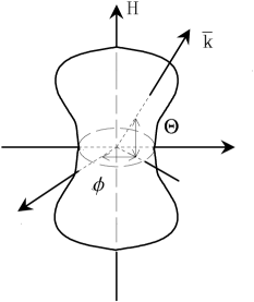
Figure 2: Spatial distribution of the cyclotron radiation produced by a single electron (see eq.16)

When the electron velocity increases the radiation field changes until at $v\approx c$, ($\mathcal{E}$ $\gg m_{e}c^{2}$) it assumes the peculiar charachters of synchrotron radiation:

i)radiated power proportional to $\mathcal{E}$ ² and $H_{p}^{2}$,

ii)continous frequency spectrum so concentrated around:

$$\omega_{m}=\omega_{o}{\displaystyle\sqrt{1-{\displaystyle v^{2}\over\displaystyle c^{2}}}\over\displaystyle 1-{\displaystyle v\over\displaystyle c}\cos\psi}~{}\propto H_{p}\mathcal{E}^{2}$$ (17)

($\psi$ is the angle between the velocity vector $\vec{v}$ and the wave vector $\vec{k}$, see fig.3), that in a given direction emission can be assumed monochromatic,

         

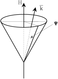
Figure 3: Velocity cone of an ultrarelativistic ($v\simeq c$) electron ($H$ = magnetic vector, $k$ wave vector, $\psi$ angle between the electron velocity and the direction of observation)

iii)radiation almost totally emitted in the forward direction of the electron motion, inside a narrow cone of aperture (see fig.4)

$$\psi\approx{\displaystyle m_{e}c^{2}\over\displaystyle\mathcal{E}}$$ (18)

Inside that cone ($\cos\psi\approx 1$) the frequency is maximum and equal to

$$\omega_{m,o}\approx\omega_{o}\left({\displaystyle{\mathcal{E}}\over\displaystyle m_{e}c^{2}}\right)^{2},$$ (19)

In the opposite direction ($\cos\psi\approx-1$) intensity and frequency are sharply reduced.

         

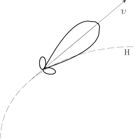
Figure 4: Distribution of the radiation emitted by an ultrarelativistic ($v\simeq c$) electron with istantaneous velocity $v$ spiralling (dashed line) around the lines of the magnetic field $H$ (orthogonal to the sheet)

iv)radiation 100 $\%$ linearly polarized when seen along the surface of the emission cone.Inside the cone the linear polarization is still dominant but a small fraction of circular polarization exists, ($V\sim o(\frac{m_{e}c^{2}}{E})$ and $I\sim U\sim Q$). Outside the cone the very small fraction of radiation produced is elliptically polarized and becomes circularly polarized when seen in directions orthogonal to the circular component of the electron spiral motion, i.e. along the $H_{p}$ direction. So the Stokes parameters depend on $H$, the angle $\mu$ between the $H$ and the line of sight, and the dimensionless frequency $\nu/\nu_{c}$, where $\nu_{c}=1.5(\omega_{m,o}/2\pi)$ is the so called critical frequency, [26],[28], itself function of $H$ (see eq.15).

b)Cloud of monoenergetic electrons

When the effects of many monoenergetic electrons with uniform distribution of pitch angles are combined, $I,Q$ and $U$ are reinforced (the Stokes parameters are additive) while $V$ is erased. In fact

$$\begin{array}[]{c}I(\nu)=c_{1}H_{p}F({\displaystyle\nu\over\displaystyle\nu_{c}})\\ {}\hfil\\ Q(\nu)=c_{2}H_{p}F_{p}({\displaystyle\nu\over\displaystyle\nu_{c}})\cos 2\chi\\ {}\hfil\\ U(\nu)=c_{2}H_{p}F_{p}({\displaystyle\nu\over\displaystyle\nu_{c}})\sin 2\chi\\ {}\hfil\\ V(\nu)\approx 0\end{array}$$ (20)

where $c_{1}$ and $c_{2}$ are constants, $F$ and $F_{p}$ frequency functions (almost monochromatic), and $\chi$ the angle between the projection of the magnetic vector on the observer plane and an axis on that plane (The projection of the magnetic vector on the observer plane is the minor axis of the polarization ellipse). When the magnetic field direction varies, the angle $\chi$ varies therefore $\cos 2\chi$ and $\sin 2\chi$ must be averaged on the magnetic field distribution along the line of sight through the cloud of emitting electrons. In conclusion the degree of polarization $p$ varies between a maximum value, (uniform magnetic field) and zero (magnetic field randomly distributed).

c)Electrons with power law energy spectrum

In the interstellar medium the radiating electrons are the cosmic ray electrons whose spectrum is a power law energy spectrum (see for instance [38], [39]) and references therein):

$$N(\mathcal{E})=K\mathcal{E}^{-\gamma}$$ (21)

where $\gamma\approx 2.4-3.0$ is the spectral index, and $K$ a normalization constant. Because the radiation produced by each electron is practically monochromatic the resulting radiation spectrum is also a power law:

$$I(\nu)=I_{0}(\gamma)H_{p}^{\frac{\gamma+1}{2}}\nu^{-\beta^{\prime}}$$ (22)

where $\beta^{\prime}=\frac{\gamma-1}{2}$ is the intensity spectral index, $\beta=\beta^{\prime}+2$ the temperature spectral index and $I_{0}$ is a slow function of $\gamma$ [26]. When the magnetic field is not uniform $H_{p}$ is replaced by $<H_{p}>$ and $I_{0}$ by a slightly different function of $\gamma$.

The Stokes parameters, products of the intensity $I(\nu)$, the degree of polarization $p$ and $\cos 2\chi$ or $\sin 2\chi$, are:

$$\begin{array}[]{c}Q=c_{3}~{}H_{p}^{\frac{\gamma+1}{2}}~{}\nu^{-\frac{\gamma-1}{2}}\cos 2\chi\\ {}\hfil\\ U=c_{3}~{}H_{p}^{\frac{\gamma+1}{2}}~{}\nu^{-\frac{\gamma-1}{2}}\sin 2\chi\\ {}\hfil\\ V\approx 0\end{array}$$ (23)

Here $c_{3}$ is a constant determined by $\gamma$ and by the magnetic field distribution along the integration path. Faraday rotation, induced by the combinations of thermal electrons (if present) and magnetic field along the line of sight through the synchrotron emitting region, usually reduces the polarization level. Moreover when the field is not uniform we have to use $<\sin 2\chi>$ and $<\cos 2\chi>$ instead of $\sin 2\chi$ and $\cos 2\chi$ so the degree $p$ of polarization decreases. Summarizing $p$ varies between 0 (random magnetic field distribution) and:

$$p_{max}={\displaystyle 3\gamma+3\over\displaystyle 3\gamma+7}<1$$ (24)

(uniform magnetic field and Faraday rotation absent).

When one looks in different directions through the interstellar medium $H$, $H_{p}=H\sin\mu$, $\chi$, $\gamma$, $\beta$ and $K$ vary (see for instance [40], [41]. Practically their values, averaged along the line of sight, behave as random variables therefore the Stokes parameters $Q_{s}$ and $U_{s}$ ($s$ stays for synchrotron) associated to the galactic (synchrotron) foreground behave as stochastic functions of the direction of observation. We can therefore write:

$$\left<Q^{2}_{s}\right>=\left<U^{2}_{s}\right>$$ (25)

It follows that for synchrotron radiation if $Q_{s}\neq 0$ also $U_{s}\neq 0$, therefore both electric and magnetic modes exist:

$$a^{E,s}\neq 0,\hskip 56.9055pta^{B,s}\neq 0$$ (26)

moreover for the synchrotron background we can write (see eqs. (13) and (25)):

$$\left<(a^{E,s})^{2}\right>=\left<(a^{B,s})^{2}\right>$$ (27)

4 CMB and its Stokes Parameters

In a homogeneous and isotropic Universe the only quantities which change as the Universe expand are temperature and intensity $I=I_{l}+I_{r}$: both decrease adiabatically. Because this is true for $I_{l}$ and $I_{r}$ separately, we do not expect anisotropy nor polarization therefore $Q=0$ and $U=I_{u}=0$ is a natural consequence.

On the contrary, inhomogeneities and perturbations of the matter density or of the gravitational field, induce anisotropy and polarization of the CMB. At the recombination epoch linear polarization is produced by the Thomson scattering of the CMB on the free electrons of the primordial plasma. The polarizarion tensor can be calculated solving the Boltzman equations, which describe the transfer of radiation in a nonstationary plasma permeated by a variable and inhomogeneous gravitational field [42], [43], [44], [15].

In our Universe the gravitational field can be divided in two parts: a background field, with homogeneous and isotropic FRW metric, and an inhomogeneous and variable mix of waves: density fluctuations, velocity fluctuations, and gravitational waves. Because of their transformation laws these waves are also said scalar, vector and tensor perturbations, respectively.

Scalar (density) perturbations affect the gravitational field, the density of matter and its velocity distribution. They were discovered by astronomers who studied the matter distribution in our Universe on scale from $\sim 1$ Mpc to $\sim 100$ Mpc. It is firmly believed they are the seeds of the large scale structure of the Universe and are reflected by the large scale CMB anisotropy detected for the first time at the beginning of the ‘90s [1], [2]. Their existence is predicted by the great majority of models of the early Universe.

Vector perturbations, associated to rotational effects, perturb only velocity and gravitational field. They are not predicted by the inflation theory and it is common believe that they do not contribute to the anisotropy and polarization of the CMB.

Tensor perturbations affect exclusively the gravitational field.

In the following we will concentrate our attention on density waves, the dominant perturbation. Because observation shows that the effects of these perturbations are small, we can treat them as small variations $\delta_{l}$, $\delta_{r}$, $\delta_{u}$ of $I_{l}$, $I_{r}$ and $I_{u}$. If we introduce the auxiliary functions $\alpha$ and $\beta$:

$$\begin{array}[]{c}\delta_{l}+\delta_{r}=(\mu^{2}-{1\over 3})\alpha,\\ {}\hfil\\ \delta_{l}-\delta_{r}=(1-\mu^{2})\beta,\\ {}\hfil\\ \delta_{u}=0,\end{array}$$ (28)

($\mu$ is the angle between the line of sight and the wave vector) and assume plane waves, the Boltzman equations (see for instance [15], [29], [30] and reference therein) become:

$$\begin{array}[]{c}{\displaystyle d\alpha\over\displaystyle d\eta}=F-{\displaystyle 9\over\displaystyle 10}\sigma_{T}n_{e}a(\eta)\alpha-{\displaystyle 6\over\displaystyle 10}\sigma_{T}n_{e}a(\eta)\beta\\ {}\hfil\\ {\displaystyle d\beta\over\displaystyle d\eta}=-{\displaystyle 1\over\displaystyle 10}\sigma_{T}n_{e}a(\eta)\alpha-{\displaystyle 4\over\displaystyle 10}\sigma_{T}n_{e}a(\eta)\beta\end{array}$$ (29)

where $F$ is the gravitational force which drives both anisotropy and polarization, $\sigma_{T}$ is the Thomson cross-section, $n_{e}$ is the density of free electrons, and $a(\eta)$ the scale factor.

These equations give:

$$\begin{array}[]{c}Q=-\frac{1}{7}(1-\mu^{2})\int F(\eta)\left(e^{-\tau}-e^{-{3\over 10}\tau}\right)d\eta\\ {}\hfil\\ U=0\end{array}$$ (30)

where $\tau(\eta)$ is the optical depth of the region where the phenomenon occurs. Rotating the coordinate system we can generate a new pair of Stokes parameters ($Q^{\prime},U^{\prime}$): no matter which is the system of reference we choose these parameters satisfy the symmetry parity condition.

Because as we saw for the CMB there is a system in which $Q\neq 0$ and $U=0$, we may conclude that magnetic modes of the CMB polarization vanish and only electric modes exist [31]. Therefore for the CMB we can write:

$$a^{E,d}\neq 0\hskip 56.9055pta^{B,d}=0$$ (31)

where index $d$ stays for density perturbation.

Concluding: in our approximation the CMB polarization is a random tensor field whose characteristcs are set by primordial density perturbations (see, for instance [45]).

5 Separation of the polarized components of Synchrotron and CMB Radiation

The CMB radiation we receive is a diffuse background which reaches us mixed with foregrounds of local origin. When the anisotropy of the CMB was detected, to remove the foregrounds from maps of the diffuse radiation, data were reorganized in the following way:

$$\hat{T}_{d}(x,y)=\hat{T}_{n}(x,y)+\hat{M}_{i}(x,y)\hat{T}_{i,c}(x,y)$$ (32)

where $\hat{T}_{d}$, is a two dimension vector (map) which gives the total signal measured at different points $(x,y)$ on the sky, $\hat{T}_{n}$ the noise vector, $\hat{M}$ the matrix which combines the components $\hat{T}_{i,c}$ of the signal. At each point $(x,y)$ we can in fact write:

$$T_{d}=g_{n}T_{n}+g_{cmb}T_{cmb,c}+g_{syn}T_{syn,c}+g_{ff}T_{ff,c}+g_{dust}T_{dust,c}+...$$ (33)

where $g_{i}$ are weights, given by $M$, $T_{syn,c}$ is the synchrotron component, $T_{ff,c}$ the free-free emission component, $T_{dust,c}$ the dust contribution and so on. Using just one map the signal components cannot be disentangled. If however one has maps of the same region of sky made at different frequencies it is possible to write a system of equations. Provided the number of maps and equations is sufficient, the system can be solved and the components of $T_{d}$ separated, breaking the degeneracy. We end up with a map of $T_{cmb}$ which can be used to estimate the CMB anisotropy.

When we look for polarization at each point on the sky we measure tensors components instead of scalar quantities, therefore to disentangle the polarized components of the CMB we need a greater number of equations. Here we will concentrate on the separation of the two dominant components of the polarized diffuse radiation: galactic synchrotron (plus dust) foreground and CMBP.

5.1 The estimator $D$

Instead of observing the same region of sky at many frequencies, we suggest a different approach. It takes advantage of the differences between the statistical properties of the two most important components of the polarized diffuse radiation (CMB (background) and synchrotron (foreground) radiation) and does not require multifrequency maps.

We define the estimator:

$$D=\left<(a^{E})^{2}\right>-\left<(a^{B})^{2}\right>$$ (34)

where $a^{E}=a^{E,s}+a^{E,d}$ and $a^{B}=a^{B,s}+a^{B,d}$ (here and in the following indexes $s$ or $d$ stay for synchrotron and density perturbations, respectively).

Because

• $E$ and $B$ modes of synchrotron do not correlate each other neither correlate with the CMB modes

  $\left<(a^{E})^{2}\right>=\left<(a^{E,s})^{2}\right>+\left<(a^{E,d})^{2}\right>+2\left<a^{E,s}a^{E,d}\right>=\left<(a^{E,s})^{2}\right>+\left<(a^{E,d})^{2}\right>$,

  $\left<(a^{B})^{2}\right>=\left<(a^{B,s})^{2}\right>+\left<(a^{B,d})^{2}\right>+2\left<a^{B,s}a^{B,d}\right>=\left<(a^{B,s})^{2}\right>+\left<(a^{B,d})^{2}\right>$,

• Electric and Magnetic modes of the CMB polarized component satisfy the condition

  $$a^{E,d}\neq 0\hskip 113.81102pta^{B,d}=0$$

• Electric and Magnetic modes $a^{E,s}$ and $a^{B,s}$, of the synchrotron radiation are both different from zero and their average values identical,

we get

$$D=\left<(a^{E,d})^{2}\right>$$ (35)

It means that $D$ provides an estimate of the contribution of the CMB to maps of the polarized diffuse radiation contaminated by galactic synchrotron emission.

Let‘ s now consider the angular power spectrum of $D$. For multipole $l$ we can write:

$$D_{l}=(a^{E}_{l})^{2}-(a^{B}_{l})^{2}={\displaystyle 1\over\displaystyle 2l+1}\sum_{m=-l}^{l}\left(|a^{E}_{lm}|^{2}-|a^{B}_{lm}|^{2}\right)$$ (36)

where $|a^{E}_{lm}|^{2}$ and $|a^{B}_{lm}|^{2}$ are random variables with gaussian distribution $p(a_{lm}^{E,B})$ (see eqs.(54) and (55) in Appendix A). According the ergodic theorem (in the limit of infinite maps, the average over 2D space is equivalent to the average over realisations) the average value of $D_{l}$ is equal to the difference of the average values of $|a^{E}_{lm}|^{2}$ and $|a^{B}_{lm}|^{2}$ summed over $m$. Taking into account equation (55) we can therefore write:

$$\left<D_{l}\right>=\left(|a^{E}_{l}|^{2}-|a^{B}_{l}|^{2}\right)$$ (37)

where :

$$\begin{array}[]{c}(a^{E}_{l})^{2}=\int\limits^{\infty}_{-\infty}|a_{lm}^{E}|^{2}p(a_{lm}^{E})d^{2}a^{E}_{lm}=\left<|a_{lm}^{E}|^{2}\right>\\ {}\hfil\\ (a^{B}_{l})^{2}=\int\limits^{\infty}_{-\infty}|a_{lm}^{B}|^{2}p(a_{lm}^{B})d^{2}a^{B}_{lm}=\left<|a_{lm}^{B}|^{2}\right>\end{array}$$ (38)

Comparing eq.38 with the ordinary definition of multipole coefficients:

$$C_{l}^{E,B}={\displaystyle 1\over\displaystyle 2l+1}\sum_{m=-l}^{l}\left<|a_{lm}^{E,B}|^{2}\right>$$ (39)

it immediately appear that we can write:

$$\begin{array}[]{c}(a^{E}_{l})^{2}=C^{E}_{l}\\ {}\hfil\\ (a^{B}_{l})^{2}=C^{B}_{l}\end{array}$$ (40)

5.2 Separation uncertainty

For synchrotron radiation $\left<D_{l}\right>$ should be zero, non zero for density perturbations, but on real maps it is always different from zero. In fact a map is just a realization of a stochastic process and the amplitudes of $|a^{E}_{lm}|^{2}$ and $|a^{B}_{lm}|^{2}$, averaged over 2D sphere, have uncertainties which add quadratically making $\left<D_{l}\right>\neq 0$ even in the case of synchrotron polarization. This effect, very similar to the well known ”cosmic variance” of anisotropy [46], [47] (the real Universe is just a realisation of a stochastic process, therefore there will be always a difference between the realization we measure and the expectation value) does not vanish if observations are repeated.

The variance of $D_{l}$ is

$${\bf V}(D_{l}^{2})=\left<D_{l}^{2}\right>-\left<D_{l}\right>^{2}$$ (41)

Being sums over $m,~{}(-l\leq m\leq+l)$ of $2l+1$ stochastic values with gaussian distribution, $a^{E}$ and $a^{B}$ have $\chi^{2}$ distributions with $2*(2l+1)$ degrees of freedom, therefore we expect their variances can be written as

$$\delta(a^{E,B})^{2}\propto\sqrt{{\displaystyle 2\over\displaystyle 2l+1}}$$ (42)

More explicitly

$$\left<D^{2}_{l}\right>={\displaystyle 1\over\displaystyle 2l+1}\left((a_{l}^{E})^{4}+(a_{l}^{B})^{4}\right)$$ (43)

and when the synchrotron foreground is dominant ($a_{l}^{E}=a_{l}^{B}$)

$$\left<D^{2}_{l}\right>={\displaystyle 2\over\displaystyle 2l+1}(a^{E}_{l})^{4}$$ (44)

in agreement with (42).

5.3 A criterium for CMBP detection

The synchrotron foreground is a sort of system noise which hampers detection of the signal, the CMB polarization. At frequencies sufficiently high ($\approx$ above 50 GHz, as we will see in the next section) the noise is small compared to the signal therefore direct detection of CMBP is possible. At low frequencies on the contrary the CMBP signal is buried in the synchrotron plus dust noise. In this case to recognize the presence of the CMB polarization we can use our estimator $D$.

At angular scale $l$, to be detectable the CMBP must satisfy the condition

$$C_{l}^{E,d}>A\cdot C_{l}^{E,s}$$ (45)

where $C_{l}^{E,i}$ are the coefficients of the multipole expansion of the $E$ modes and $A$ is the confindence level of the signal detectability. In a similar way we can write for our estimator:

$$D_{l}^{E,d}>A\cdot D_{l}^{E,s}$$ (46)

where, as we said before, $D_{l}^{E,d}=C_{l}^{E,d}$ and

$$D_{l}^{E,s}=\sqrt{{\displaystyle 2\over\displaystyle 2l+1}}(a_{l}^{E,s})^{2}$$ (47)

Therefore, the criterium for the CMBP detection becomes

$$D_{l}^{E,d}\geq A\cdot\sqrt{{\displaystyle 2\over\displaystyle 2l+1}}C_{l}^{E,s}$$ (48)

This means that using D we can recognize CMBP in a map of the polarized diffuse radiation with an uncertainty  $\simeq\sqrt{{\displaystyle 2\over\displaystyle 2l+1}}C_{l}^{E,s}$ which decreases as $l$ and angular resolution increases.

6 Angular power spectra of polarized synchrotron.

The angular power spectra of the polarized component of the synchrotron radiation have been discussed by [48], [49], [50], [51] and [52]. It appears that the power spectra of the degree of polarization $p$ and of electric and magnetic modes $E$ and $B$ follow power laws up to $l\sim 10^{3}$. The spectral index of the power law which holds for the degree of polarization is $\alpha_{p}\simeq 1.6-1.8$. For the $E$ and $B$ modes different authors get from the observations values of the spectral index different, but marginally consistent. In paper [51] and [52], using Parkes data, the authors get

$$C^{E,B}_{l}\sim C_{0,E,B}\left({\displaystyle l_{0}\over\displaystyle l}\right)^{\alpha_{E,B}}$$ (49)

with $\alpha_{E}\approx\alpha_{B}\approx 1.4\div 1.5$ and dependence of $\alpha$ on the sky region and the frequency.

In paper [48], using Effelsberg and Parkes data, the authors get:

$$C^{E,B}_{l}=C_{0}\cdot 10^{-10}\left({\displaystyle 450\over\displaystyle l}\right)^{\alpha}\cdot\left({\displaystyle 2.4\mbox{GHz}\over\displaystyle\nu}\right)^{2\beta}$$ (50)

with $\alpha=(1.8\pm 0.3)$, $\beta=2.9$ and $C_{0}=(1.6\pm 1)$ (here we modified the original expression given in [48] writing it in adimensional form). As said above the spectral indexes $\alpha$ obtained by [51] [52] and [48] are marginally consistent.

Both authors got their results analyzing low frequency data (1.4, 2.4 and 2.7 GHz), therefore the extension of their spectra to tens of GHz, the region where CMB observations are usually made, depend on the accuracy of $\beta$, the temperature spectral index of the galactic synchrotron radiation. A common choice is $\beta=2.9$ but in literature there are values of $\beta$ ranging between $\approx 2.5$ and $\approx 3.5$. Moreover $\beta$ depends on the frequency and the region of sky where measurements are made (see [38], [53], [54], [55]). Finally the values of $\beta$ in literature have been obtained measuring the total (polarized plus unpolarized) galactic emission. In absence of Faraday effect $\beta,\beta_{pol}$ and $\beta_{unpol}$, the spectral indexes of the total, polarized and unpolarized components of the galactic emission, are identical (see eqs. (22),(23)). However when Faraday effect with its $\nu^{-2}$ frequency dependence is present, we expect that, as frequency increases, the measured value of the degree of polarization (se eq. (24)) increases, up to

$$p\leq p_{max}={\displaystyle 3\beta-3\over\displaystyle 3\beta-1}$$

therefore we should measure $\beta_{pol}\leq\beta$. The expected differences are however well inside the error bars of the available data therefore at present we can neglect differences and set $\beta\simeq\beta_{pol}\simeq\beta_{unpol}$.

Instead of extrapolating low frequency results it would be better to look for direct observations of the galactic emission and its polarized component at higher frequencies. Unfortunately above 5 GHz observations of the galactic synchrotron spectrum and its distribution are rare and incomplete. At 33 GHz observations by [56] give for some patches on the sky a galactic temperature of about $2\div 4\mu K$ from which follows that at the same frequency we can expect polarized foreground signals up to several $\mu K$. At 14.5 GHz observations made at OVRO [57] give synchrotron signals of 175 $\mu K$, equivalent to about 15 $\mu K$ at 33 GHz of which up to 10 $\mu K$ can be polarized.

In conclusion there are large uncertainties when one try to decide at which frequency the polarized component of the galactic diffuse emission does not disturb observation of the CMB. To be on the safe side we can say, and all the authors of papers [48], [49], [50], [51] and [52] agree, that the CMB polarized component surely overcomes the polarized synchrotron foreground only above 50 GHz, therefore direct observations of the CMB are better made at frequencies greater of 50 GHz. Below 50 GHz observations of CMBP are problematic because the contamination by galactic polarized emission can be high and its evaluation, usually by multifrequency observations, not sure.

         

Figure 5: Power spectrum versus multipole order $l$ of the polarized components of CMB (solid line) and three possible power spectra of the galactic synchrotron radiation ($\alpha=1.5$ (dotted line), $\alpha=1.8$ (dashed line) and $\alpha=2.1$ (dot-dash line)) calculated at 43 GHz. (See text for details of calculations and model)

This conclusion is supported by figure 5. It shows plots versus the multipole order $l$ of the power spectra of the polarized components of CMB and galactic synchrotron calculated at 43 GHz. The CMB spectrum has been obtained using CMBFAST [58] and standard cosmological conditions (CMB power spectrum normalized to the COBE data at low $l$, $\Omega_{b}=0.05$, $\Omega_{CDM}=0.3$ , $\Omega_{\Lambda}=0.65$, $\Omega_{\nu}=0$, $H_{0}=65$ km/sec/Mpc, $T_{CMB}=2.726K$ , $Y_{He}=0.24$, standard recombination). The synchrotron spectrum has been calculated assuming for $E_{l}$ and $B_{l}$ the scaling law (50) with $C_{0}=2.6$ (most pessimistic case), and $\alpha=1.5;~{}1.8;~{}2.1$ and $\beta=2.9$ respectively. At this frequency (43 GHz) the CMB power becomes comparable to the synchrotron power only at very small angular scales ($l\geq 500$).

Similar calculations at other frequencies confirm that only above $\simeq 50$ GHz and at small angular scales (large values of $l$) the CMBP power spectrum overcomes the synchrotron spectrum. Below $\simeq 50$ GHz the CMBP power is always below the power level of synchrotron therefore CMBP detection is impossible even at small angular scale.

We can however overcome this limit and plan CMBP observations at lower frequencies if we use our estimator. To see how it improves the CMBP detectability we calculate the angular power spectrum of $D^{s}_{l}$, the estimator we expect when the diffuse radiation is completely dominated by synchrotron galactic emission. Combining eqs.(39), (44) and (50) we can write:

$$\sqrt{\left<(D^{s}_{l})^{2}\right>}=C_{0}\cdot 10^{-10}\sqrt{{\displaystyle 2\over\displaystyle 2l+1}}\left({\displaystyle 450\over\displaystyle l}\right)^{\alpha}\cdot\left({\displaystyle 2.4\mbox{GHz}\over\displaystyle\nu}\right)^{2\beta}$$ (51)

This quantity can be directly compared with the power spectrum of CMBP because as we saw (see eqs.(31), (37), (40) and (43), $D^{d}_{l}$ the power spectrum of the estimator evaluated when the sky is dominated by CMBP coincides with the CMBP power spectrum.

Figure 6 shows the power spectra at 37 GHz of i)$D^{s}_{l}$ the estimator for a galactic synchrotron dominated sky (solid line), calculated using eq.(50), ii)$D^{d}_{l}$ the estimator for a CMBP dominated sky which coincides with the power spectrum of CMBP (dotted line) calculated as in figure 5 with CMBFAST using the same standard cosmological conditions, iii)the power spectrum of the polarized component of the galactic synchrotron radiation (dashed line), calculated using eq.(50). As expected at 37 GHz the CMBP power level is well below the level of synchrotron power, therefore direct observations of CMBP are impossible (the maximum value of the CMBP power is about 2.5 times smaller than the synchrotron power at the same $l$). However above $l\simeq 250$ the power associated to the synchrotron estimator is definitely below the power associated to the CMBP estimator with a maximum ratio CMBP/D $\sim 7$ at $l=1000$. This confirms that the use of $D$ allows to recognize the CMBP also at frequencies well below 50 GHz.

Figure 6: Power spectrum at 37 GHz of the expected value of the estimator for a galactic synchrotron dominated sky (solid line). The dotted line represents both the estimator and the CMBP power spectrum for a CMBP dominated sky. The dashed line is the power spectrum of the polarized component of the galactic synchrotron radiation (dashed line) (see text for details of model and calculations)

7 Simulation

To further test the capability of our estimator we studied the separation of CMB and galactic synchrotron during observations using, instead of the expected values of $D_{l}$, as we did in figure 6, measured values simulated by random series of numbers, with gaussian distribution $\sim N(0,1)$, zero mean and unity variance (see eqs (54) - (55)). To simulate measurements we generate $2l+1$ random numbers to represent $a^{E}_{lm}$ and $2l+1$ random numbers to represent $a^{B}_{lm}$. We then use these values to work out $D_{l}$ using eq.(36).

         

Figure 7: Multipole power spectrum of simulated measurements of the estimator $D$ for a synchrotron dominated sky (see text) with infinite angular resolution (no smoothing on $l$, ($\Delta l=1$))

Because of their finite angular resolution observations include an average of the signal on regions whose angular extension cover a finite multipole interval $\Delta l$. For instance Boomerang data come from regions whose angular extension is equivalent to $\Delta l\sim 100$ [3], [4], [5]. To get more realistic data we averaged $D_{l}$ on an interval $\Delta l=n$:

$$\hat{D}_{l}={\displaystyle 1\over\displaystyle n+1}|\sum\limits_{k=0}^{k=+n}D_{l-n/2+k}|$$ (52)

Figure 7, figure 8 and figure 9 give plots of $|\hat{D}_{l}|$ (the sign of $D_{l}$ is arbitrary) versus $l$, for $\Delta l=1$, $\Delta l=10$ and $\Delta l=100$ respectively: the very large fluctuations of the estimator one observes when $\Delta l=1$, above $l\simeq 400$ are drastically reduced as soon as $\Delta l$ increases. The smoothing effect of the average can be appreciated comparing figure 7, figure 8 and figure 9 where $\hat{D}_{l}$ is plotted for $n=1$, $n=10$ and $n=100$ respectively:

         

Figure 8: Same as figure 7 with finite angular angular (smoothing on $\Delta l=10$)

         

Figure 9: Same as figure 7 with finite angular resolution (smoothing on $\Delta l=100$)

Figure 10, figure 11 and figure 12 are similar to figure 10 and plot at 37 GHz, instead of the expectation value of $D^{s}_{l}$, simulated measurements of it, for $\Delta l=1$ (figure 10), $\Delta l=10$ (figure 11) and $\Delta l=100$ (figure 12), respectively. Once again the CMBP power spectrum has been calculated with CMBFAST assuming the same cosmological conditions we assumed above and the synchrotron power spectrum comesfrom eq.(50) with $C_{o}=2.6,\alpha=1.5,\beta=2.9$ (most pessimistic condition).

         

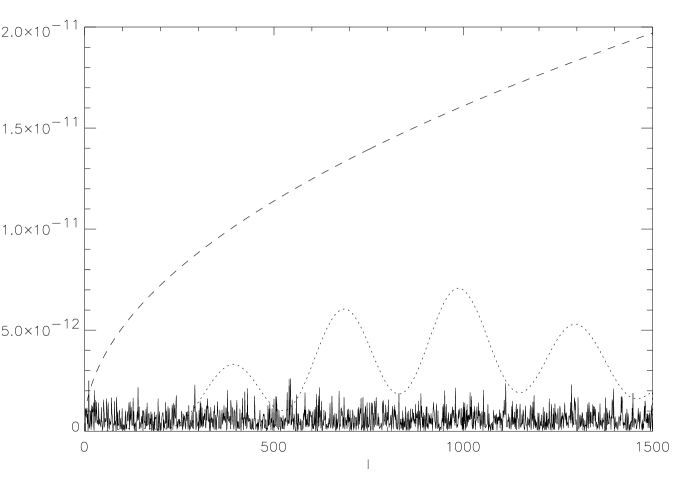
Figure 10: Similar to figure 6. Here we plot simulated measurements with infinite angular smoothing resolution (no smoothing on $l$) instead of the expectation value of the estimator at 37 GHz for a synchrotron dominated sky. The dotted line give both the estimator and the CMBP power spectrum for a CMBP dominated sky. The dashed line is the power spectrum of the galacic synchrotron when its expected contribution is maximum (eq. (50) with $\beta=2.9$, $\alpha=1.5$ and $C_{o}=2.6$) (see text for details)

         

Figure 11: Same as figure 10 with finite angular resolution (smoothing on $\Delta l=10$)

         

Figure 12: Same as figure 10 with finite angular resolution (smoothing on $\Delta l=100$)

Figure 13 is the same of figure 12 at a much lower frequency, 17 GHz. Here on the vertical axis we used logarithmic instead of linear scale, which allows a better appreciation of the differences among the three curves. The estimator power spectrum now almost touches the two highest peaks of the CMBP spectrum. Therefore, 17 GHZ is probably the lowest frequency at which one can hope to detect CMBP using $D_{l}$, in the most favorable conditions. In the most pessimistic case ($C_{0}=2.6$ and $\alpha=1.5$) the corresponding frequency is 25 GHz.

         

Figure 13: Same as figure 12 at 17 GHz using logarithmic scale on the vertical axis

8 Conclusions

Observations of the CMB polarization are hampered by the presence of the galactic polarized foreground. Only above $\sim 50GHz$ the cosmic signal is definitely above the galactic synchrotron and direct observations of CMBP are, in principle, possible. Between $\sim 30$ GHz and $\sim 50$ GHz the level of the polarized component of the synchrotron foreground is at least comparable to the CMBP level, but the observational situation is still insufficient to evaluate precisely its contribution to maps of the diffuse polarized radiation measured by a telescope. Below $\sim 30$ GHz the galactic signal is definitely dominant. So far a common approach for studies of CMBP was to make accurate maps of the diffuse polarized radiation from a given region of sky at many frequencies and disentangle the various contributions modelling their frequency dependence and spatial distribution.

We have shown that an alternative way is to take advantage of the different statistical properties of the spatial distribution of the main components of the polarized diffuse radiation: CMBP and synchrotron (plus dust) galactic foreground. By measuring the $E$ and $B$ modes of the polarized radiation we can build an estimator which improves the background/foreground ratio by a factor sufficient to allow firm recognition and extraction of the CMBP contribution from single frequency maps at least down to 25 GHz (17 GHz in the most favorable conditions) at angular scales $\leq 0.7^{o}$ ($l\geq 250$).

Appendix: stochastic properties of harmonics amplitudes

Here and overall in paper we suppose that $a_{lm}^{s}$ are complex random variables which satisfy the probability distribution law:

$$\begin{array}[]{c}p(a_{lm}^{E})={\displaystyle 1\over\displaystyle\pi E_{l}^{2}}exp\left(-{\displaystyle|a_{lm}^{E}|^{2}\over\displaystyle E^{2}_{lm}}\right)\\ {}\hfil\\ p(a_{lm}^{B})={\displaystyle 1\over\displaystyle\pi B_{l}^{2}}exp\left(-{\displaystyle|a_{lm}^{B}|^{2}\over\displaystyle B^{2}_{lm}}\right)\end{array}$$ (53)

with variance $\left<|a^{E}_{lm}|^{2}\right>=E^{2}_{l}$ and $\left<|a^{B}_{lm}|^{2}\right>=B^{2}_{l}$.

They have all the propertiers of gaussian variables (below we omitt indexes $E$ and $B$ in first and second equations):

$$\begin{array}[]{c}\int\limits_{-\infty}^{\infty}p(a_{lm})d^{2}a_{lm}=1\\ {}\hfil\\ \int\limits^{\infty}_{-\infty}a_{lm}p(a_{lm})d^{2}a_{lm}=0\end{array}$$ (54)

$$\begin{array}[]{c}\int\limits^{\infty}_{-\infty}|a_{lm}^{E}|^{2}p(a_{lm}^{E})d^{2}a^{E}_{lm}=E^{2}_{l}\\ {}\hfil\\ \int\limits^{\infty}_{-\infty}|a_{lm}^{B}|^{2}p(a_{lm}^{B})d^{2}a^{B}_{lm}=B^{2}_{l}\end{array}$$ (55)

Setting

$$\left<F\right>=\int\limits^{\infty}_{-\infty}Fp(a_{lm})d^{2}a_{lm}$$ (56)

with current index $E$ or $B$, it immediately follows:

$$\begin{array}[]{c}\left<|a_{lm}^{E}|^{4}\right>=\int\limits^{\infty}_{-\infty}|a_{lm}^{E}|^{4}p(a_{lm}^{E})d^{2}a^{E}_{lm}=2E^{4}_{l}\\ {}\hfil\\ \left<|a_{lm}^{B}|^{4}\right>=\int\limits^{\infty}_{-\infty}|a_{lm}^{B}|^{4}p(a_{lm}^{B})d^{2}a^{B}_{lm}=2B^{4}_{l}\end{array}$$ (57)

References

- [1] Strukov, I.A., et al.,1992: Mon. Not. R. Astron. Soc. 258, 37P.
- [2] Smoot, G., et al., 1992: ApJ 396, L1.
- [3] de Bernardis, P.,et al., 2000: Nature 404, 955.
- [4] de Bernardis, P.,et al., 2002: ApJ 564, 559.
- [5] Netterfield, C.B., et al., 2002: ApJ 571, 604.
- [6] http://map.gsfc.nasa.gov and references therein
- [7] Delabrouille J. and Kaplan J. 2002: AIP Conf. Proc. 609, 135.
- [8] Villa F. et al. 2002: AIP Conf. Proc. 609, 150
- [9] Kesteven M. 2002: AIP Conf. Proc. 609, 156
- [10] Piccirillo L. et al. 2002: AIP Conf. Proc. 609, 159.
- [11] Gervasi M. et al. 2002: AIP Conf. Proc. 609, 164
- [12] Masi S. et al. 2002: AIP Conf. Proc. 609, 129
- [13] S.Cortiglioni et al., 1999: AIP Conf. Proc. 476, 1999, p.186.
- [14] Rees, M.J., 1968: ApJ 153, L1.
- [15] Sazhin M.V., Benitez N., 1995: Astrophys. Lett. Commun. 32, 105.
- [16] Ng K.L., Ng K.W., 1996: ApJ 456, 413.
- [17] Melchiorri A., Vittorio N., 1997: in: The Cosmic Microwave Background, NATO ASIC Proc. 502, 419.
- [18] Prunet, S., Sethi, S.K., Bouchet, F.R., 1998: A&A 339, 187.
- [19] Fosalba P., Lazarian A., Prunet S., Tauber J.A., 2002: AIP Conf. Proc. 609, 44.
- [20] Dodelson, S., 1997: Ap.J. 482, 577.
- [21] Tegmark, M., 1999: Ap.J. 519, 513.
- [22] V. Stolyarov, M. P. Hobson, M. A. J. Ashdown, A. N. Lasenby, 2002: Mon. Not. R. Astron. Soc., in press.
- [23] Tegmark, M., Efstathiou G., 1996: Mon. Not. R. Astron. Soc. 281, 1297.
- [24] Kogut A., Hinshaw G., 2000: ApJ 543, 530.
- [25] M.V. Sazhin, 2002: AIP Conf. Proc. 609, 66.
- [26] Ginzburg V.L., Syrovatskii S.I., 1965: Ann. Rev. Astron. Astrophys. 3, 297.
- [27] Gardner F.F., Whiteoak J.B., 1966: Ann. Rev. Astron. Astrophys. 4, 45.
- [28] Ginzburg V.L., Syrovatskii S.I., 1969: Ann. Rev. Astron. Astrophys. 7, 375.
- [29] Sazhin M.V., and Shulga V.V., Vestnik MSU, 1996: Moscow State University, Moscow ser.3, N 3, p. 69.
- [30] Sazhin M.V., and Shulga V.V., Vestnik MSU, 1996: Moscow State University, Moscow ser.3, N 4, p. 87.
- [31] Seljak U., Zaldarriaga M., 1997: Phys.Rev.Lett. 78, 2054.
- [32] Goldberg, J.N., et al., 1967: J. Math. Phys. 8, 2155.
- [33] Gelfand, I.M., Minlos, R.A., Shapiro, Z, Ya., 1958: The Representation of the rotation group and the Lorenz group. FizMatGiz Publ., Moscow, 1958.
- [34] Zerilli, F. J., 1970: J. Math. Phys. 11, 2203.
- [35] Thorn, K.S., 1980: Rev. Mod. Phys. 52, 299.
- [36] Sazhin, M.V., Sironi, G., 1999: New Ast. 4, 215.
- [37] Westfold K.S., 1959: ApJ 130, 241.
- [38] Gavazzi G. and Sironi G. 1975: Rivista del Nuovo Cimento 5, 155
- [39] Longair M.S., 1994: High Energy Astrophysics, CU Press, Cambridge (UK)
- [40] Wielebinski, R., 2002: AIP Conf. Proc. 609, 90.
- [41] W. Reich, E. Fuerst, P. Reich, R. Wielebinski, M. Wolleben, 2002: AIP Conf. Proc. 609, 3.
- [42] Basko, M.M., Polnarev, A.G., 1980: Mon.Not.R.Astron.Soc. 191, L47.
- [43] Sazhin, M.V., 1984: Modern Theoretical and Experimental Problems of General Relativity and Gravitation, Moscow Pedagogical Inst. Publ., Moscow, 1984, p. 88.
- [44] Harrari, D., Zaldarriaga, M., 1993: Phys.Lett. B 319, 96.
- [45] Dolgov, A. D., Sazhin, M. V., Zeldovich, Ya. B. 1990: in Basics of modern cosmology, Editions Frontieres, Gif -Sur -Yvette, pag 251.
- [46] Knox, L., Turner, M.S., 1994: Phys.Rev.Lett 73, 3347.
- [47] Sazhin, M.V., Bryukhanov, A.A., Strukov, I.A., Skulachev, D.P., 1995: Astronomy Letters 21, 358.
- [48] Baccigalupi, C., Burigana, C., De Zotti G., Perotta F., 2002: AIP Conf. Proc. 609, 84.
- [49] Burigana C., and La Porta L., 2002: AIP Conference Proc. vol. 609,
- [50] Tucci, M., Caretti, E., Cecchini, S., Fabbri.,R., Orsini M., Pierpaoli E., 2002: New Ast. 5, 181.
- [51] Tucci, M., Caretti, E., Cecchini, S., Nicastro, L., Fabbri., R., Gaensler, B.M., Dickey, J.M., McClure-Griffiths N.M., 2002: AIP Conf. Proc. 609, 60
- [52] Bruscoli, M., Tucci, M., Natale, V., Carretti, E., Fabbri, R., Sbarra, C., Cortiglioni, s., 2002: New Ast. 7, 171
- [53] Salter C.J. and Brown R.L. 1988: in Galactic and Extragalactic Radio Astronomy, Verschuur G.L. and Kellermann K.I. Eds., Springer Verlag , Berlin, pag. 1.
- [54] Zannoni M. et al. 2000: in New Cosmol. Data and the values of Fundamental Param., IAU Symp. 201 : in press
- [55] Platania P., et al. 1998: ApJ 505, 473
- [56] Davies R.D., Wilkinson A., 1998: in Fundamental patrameters in Cosmology, Ed. Frontieres, Gif sur Yvette 1998, pag. xxxx and Davies R.D., Wilkinson A., 1999: ASP Conf.181, 77.
- [57] Mukherjee, P., Dennison, B., Ratra, B., Simonetti, John II, Ganga, K., Hamilton, J.C., 2003: Ap.J in press.
- [58] Seljak, U., Zaldarriaga, M., http:// physics.nyu.edu/ matiasz/ CMBFAST/ cmbfast.html.