THE INFLUENCE OF MAGNETIC FIELDS ON THE SUNYAEV-ZEL’DOVICH EFFECT IN CLUSTERS OF GALAXIES

Abstract

We study the influence of intracluster large scale magnetic fields on the thermal Sunyaev-Zel’dovich (SZ) effect. In a macroscopic approach we complete the hydrostatic equilibrium equation with the magnetic field pressure component. Comparing the resulting mass distribution with a standard one, we derive a new electron density profile. For a spherically symmetric cluster model, this new profile can be written as the product of a standard ($\beta$-) profile and a radius dependent function, close to unity, which takes into account the magnetic field strength. For non-cooling flow clusters we find that the observed magnetic field values can reduce the SZ signal by $\sim 10\%$ with respect to the value estimated from X-ray observations and the $\beta$-model. If a cluster harbours a cooling flow, magnetic fields tend to weaken the cooling flow influence on the SZ-effect.

, ,

1 Introduction

The SZ-effect is rapidly turning into an important astrophysical tool thanks to the progress of the observational techniques, which allow increasingly precise measurements. In view of these developments it is thus relevant to study further corrections to it, such as relativistic effects (Rephaeli, 1995), the shape of the galaxy cluster and its finite extension or a polytropic temperature profile (see e.g. Puy et al. (2000)), corrections induced by halo rotation (Cooray and Chen, 2001), Brillouin scattering (Sandoval-Villalbazo and Maartens, 2002), early galactic winds (Majumdar et al., 2001) and the presence of cooling flows (Schlickeiser, 1991; Majumdar et al., 2001). These additional effects are of different relevance and often depend on the specific cluster values.

Whereas, e.g. cooling flows are not present in every cluster of galaxies, the need for relativistic corrections due to energetic non-thermal electron populations seems to be common in most clusters. (Blasi et al., 2000; Shimon and Rephaeli, 2002). These relativistic electrons produce a hard X-ray component in excess of the thermal spectrum by Compton scattering off the Cosmic Microwave Background (CMB) and by non-thermal bremsstrahlung. Their emission has been quite possibly detected in Coma (Rephaeli et al., 1999; Fusco-Femiano et al., 1999), A2199 (Kaastra et al., 1999), A2256 (Molendi et al., 2000) and A2319 (Gruber and Rephaeli, 2002) by RXTE and BeppoSAX satellites. The main evidence for the existence of relativistic electrons comes from radio synchrotron emission of extended intracluster regions (Giovannini et al., 1999; Giovannini and Feretti, 2000) and is, therefore, closely related to the presence of magnetic fields. The magnetic fields in the intracluster gas lead to acceleration processes and modify the classical Maxwell-Boltzmann distribution of the electrons, which might acquire a significantly non-thermal spectrum and thus account for the observed hard X-ray spectra (Ensslin et al., 1999; Blasi, 2000). Consequently, several authors (Rephaeli, 1995; Itoh et al., 1998; Challinor and Lasenby, 1998; Birkinshaw, 1999) derived relativistic corrections to the thermal SZ-effect up to different leading orders. Though the magnetic field is related to the relativistic electron population, its own influence - as a non-thermal cluster component - on the SZ-effect has not yet been investigated. Whereas the importance of relativistic corrections to the SZ-effect depends on the cluster temperature, the magnetic field seems to be ubiquitous with a mean field value of $5-10\,\mu G$ in the cluster cores (Clarke et al., 2001). Independently of the diffuse non-thermal radio emission, excess Faraday rotation measure of polarized radio emission in radio sources within or behind the cluster can prove the existence of magnetic fields. This method was applied to the Coma cluster, where Feretti et al. (1995) found a large magnetic field of $B\geq 8.3\,\mu G$. Govoni et al. (1999) found a similar value ($5-10\,\mu G$) for A119. Clarke et al. (1999) derived magnetic field strengths of a few $\mu G$ for their cluster sample by using a statistical Faraday rotation measure technique. Unfortunately, the structure of the magnetic field is presently poorly known. Contrary to the static situation in non-cooling flow clusters, the magnetic field is believed to become dynamically significant in the cores of cooling flow clusters (Eilek and Owen, 2001). Taylor et al. (2001) found a magnetic field strength of up to $40\,\mu G$ in the Centaurus cluster. The converging cooling flow (see e.g. Fabian et al. (1991); Fabian (1994)) causes a compression and enhancement in the magnetic field strength and finally reconnection might transfer the magnetic energy back to the plasma when the magnetic field pressure becomes comparable to the thermal gas pressure.
As the ratio of the magnetic pressure ($P_{B}$) to the gas pressure ($P_{g}$) reaches $\frac{P_{B}}{P_{g}}\sim 10^{-2}$ for the quoted values of non-cooling flow clusters and even unity for the cores of cooling flow clusters, we consider the additional magnetic field pressure term to be significant and we will examine its influence on the SZ-effect. We remark that all the quoted values refer to large scale magnetic fields with a coherence length of typically $1-10\,kpc$. There are essentially no useful limits on the strength of any small scale magnetic fields. Our calculation is based on a macroscopic picture inferred from the existence of this additional (large scale) pressure component and we do not start our considerations at the level of the single particle movement in a magnetic field. The current cluster data reveal magnetic field values which result to be significant for a correct SZ analysis, especially towards the cluster core where the electron density increases.

The aim of the paper is to examine the influence of large scale magnetic fields on the thermal SZ-effect. We, therefore, choose a phenomenological approach, where the addition of a magnetic field pressure to the gas pressure is well justified. For a given magnetic field model, we can then estimate the change in the electron density and the temperature profiles as compared to standard ones used in the literature in the absence of magnetic fields.

The paper is organised as follows: In section 2 we present the theoretical model for the magnetic field contribution. We derive new gas density profiles which are then used to calculate the SZ-effect. We distinguish two situations according to whether a cluster harbours a cooling flow or not. Section 3 shows our results and contains a discussion of how magnetic fields influence the SZ signal and what are the observational consequences. As an illustration we apply our results to the non-cooling flow cluster A119. Our conclusions are given in section 4.

2 Magnetic field contribution

2.1 Non-cooling flow clusters

We suppose a standard spherically symmetric model for a cluster, which is assumed to be in a relaxed state with a static gravitational potential. Thus, hydrostatic equilibrium can be expected. The intracluster plasma is treated as an ideal gas and thus the well known hydrostatic equilibrium equation has the form (see e.g. Sarazin (1988)):

$$\frac{1}{\rho_{g}(r)}\frac{dP_{g}(r)}{dr}=-\frac{G\,\mathcal{M}(r)}{r^{2}},$$ (1)

where $G$ is the gravitational constant, $\rho_{g}(r)$ and $P_{g}(r)$ are the radius dependent gas density and pressure, respectively, and $\mathcal{M}(r)$ is the gravitating mass within the radius $r$. $\mathcal{M}(r)$ is mainly determined by the dark matter profile, whereas the gas mass contribution is negligible. When taking into account magnetic fields, the hydrostatic equilibrium Eq.(1) has to be completed with a magnetic hydrostatic pressure term $P_{B}$ of the form:

$$P_{B}(r)=\frac{B^{2}(r)}{8\pi},$$ (2)

where $B(r)$ is the magnetic field strength, which is supposed to be spherically symmetric. Thus, the magnetic field contributes to the total pressure opposing the gravitational force. The gas pressure $P_{g}(r)$ in Eq.(1) is replaced by the sum of gas and magnetic field pressure:

$$P_{g}(r)+P_{B}(r)=\frac{k}{\mu\,m_{p}}\rho_{g}(r)T_{g}(r)+\frac{B^{2}(r)}{8\pi},$$ (3)

where $k$ is the Boltzmann constant, $\mu$ the mean molecular weight, $m_{p}$ the proton mass and $T_{g}(r)$ the gas temperature at radius $r$.
When deriving the mass distribution from Eq.(1), either with only the gas pressure or with the magnetic field pressure added as in Eq.(3), we obviously end up with the two different equations:

$$\mathcal{M}(r) = -\frac{k\,T_{g}(r)}{G\,\mu\,m_{p}}r\left[\frac{d\ln\rho_{g}(r)}{d\ln r}+\frac{d\ln T_{g}(r)}{d\ln r}\right],$$ (4)

$$\mathcal{M}_{B}(r) = -\frac{k\,T_{B}(r)}{G\,\mu\,m_{p}}r\left[\frac{d\ln\rho_{B}(r)}{d\ln r}+\frac{d\ln T_{B}(r)}{d\ln r}\right]-\frac{r^{2}}{G\,\rho_{B}(r)}\frac{dP_{B}(r)}{dr},$$ (5)

where $T_{B}(r)$ and $\rho_{B}(r)$ describe the gas temperature and density, respectively, in the presence of the magnetic field.

As next we compare the Eqs.(4) and (5). To find the cluster mass distribution we can either proceed our analysis according to Eq.(4) or, if we take into account magnetic fields, according to Eq.(5). However, the true total gravitating cluster mass is unique and must be the same, thus $\mathcal{M}_{B}(r_{l})\equiv\mathcal{M}(r_{l})$, $r_{l}$ being the cluster limiting extension. Nevertheless, $T_{B}(r)$ and $\rho_{B}(r)$ can be different from $T_{g}(r)$ and $\rho_{g}(r)$ due to the magnetic field pressure gradient. In what follows, we want to relate $\rho_{B}(r)$ to $\rho_{g}(r)$, which is supposed to be known and to be a correct theoretical description for the gas density profile in absence of magnetic fields (e.g. $\beta$-model, Sarazin (1988)).
As dark matter is the dominant mass component in clusters of galaxies (up to $80-90\%$ of the total mass) and supposed not to be affected by magnetic fields, we expect in good approximation the equality between the Eqs.(4) and (5) to be satisfied for all radii $r$:

$$\mathcal{M}_{B}(r)=\mathcal{M}(r).$$ (6)

Clearly, this approximation is justified as long as the density profiles $\rho_{B}(r)$ and $\rho_{g}(r)$ do not differ substantially. As we will see, our results do indeed satisfy this requirement. For the sake of simplicity we assume isothermal temperature profiles: $T_{g}(r)\equiv T_{g}$, $T_{B}(r)\equiv T_{B}$. By setting equal the right hand sides of the Eqs.(4) and (5), we find a first order differential equation for $\rho_{B}(r)$, which yields:

$$\rho_{B}(r)=\rho_{g}(r)^{\frac{T_{g}}{T_{B}}}\rho_{g,0}^{1-\frac{T_{g}}{T_{B}}}\left[1+\rho_{g,0}^{\frac{T_{g}}{T_{B}}-1}\Big{(}\frac{\mu\,m_{p}}{k\,T_{B}}\Big{)}\int\limits_{r}^{r_{l}}\frac{P^{\prime}_{B}(\tilde{r})}{\rho_{g}(\tilde{r})^{\frac{T_{g}}{T_{B}}}}\,d\tilde{r}\right],$$ (7)

where prime is the derivative with respect to $r$ and $\rho_{g,0}$ is the central gas density. The boundary condition is chosen to be $\rho_{B}(r_{l})=\rho_{g}(r_{l})$ for $r_{l}$ at the cluster limiting radius, where the magnetic field is negligible. Physically, we do not expect the temperatures $T_{g}$ and $T_{B}$ to differ significantly. Thus, in the sense of a first order development, we suppose $T_{g}$ and $T_{B}$ to be approximately equal, which simplifies the above equation. Mathematically, the boundary condition and the assumption of isothermal temperature profiles even impose $T_{B}\equiv T_{g}$: At the limiting radius $r_{l}$, the magnetic field pressure gradient in Eq.(5) vanishes and the densities are then equal. As the temperatures are isothermal, the second term in brackets in the Eqs.(4) and (5) drops, stating that $T_{B}=T_{g}$ at $r_{l}$, which is then also true for the whole cluster.

To evaluate Eq.(7) we need a magnetic field model. Various physical models have been invoked to explain the rotation measure in radio sources in clusters of galaxies (Jaffe, 1980; Tribble, 1991). According to them, the magnetic field distribution is correlated with the electron density of the thermal gas. Recently, Dolag et al. (2001), based upon a correlation between X-ray surface brightness and Faraday rotation measure, derived the following relation:

$$B(r)\propto(n_{e}(r))^{\gamma},$$ (8)

where $n_{e}(r)$ is the electron number density and $\gamma$ the slope of the $B-n_{e}$ relation, which depends on the specific cluster of galaxies. They showed, that Eq.(8) can be motivated by both simulations and observational data. Furthermore, they clearly excluded the possibility of a constant magnetic field through the intracluster medium. With the relation (8) the magnetic field profile is proportional to $\rho_{B}(r)$ and we can thus rewrite Eq.(7) as follows:

$$\rho_{B}(r)=\rho_{g}(r)\left[1+\frac{1}{\rho_{B,0}^{\,\,2\gamma}}\frac{B_{0}^{\,2}}{8\pi}\Big{(}\frac{\mu\,m_{p}}{k\,T_{g}}\Big{)}\int\limits_{r}^{r_{l}}\frac{(\rho_{B}^{\,\,2\gamma})^{\prime}(\tilde{r})}{\rho_{g}(\tilde{r})}\,d\tilde{r}\right],$$ (9)

where $\rho_{B,0}$ and $B_{0}$ are the cluster central gas density and the central magnetic field value, respectively. Eq.(9) is an integro-differential equation for $\rho_{B}(r)$. It expresses the modified density $\rho_{B}(r)$ as the standard density $\rho_{g}(r)$ from Eq.(4), multiplied with a radius dependent function which involves the magnetic field pressure. As in perturbation theory, $\rho_{B}(r)$ can also be interpreted as the product of the unperturbed quantity $\rho_{g}(r)$ multiplied by the function in brackets in Eq.(9), which is close to unity. Following an iterative procedure to solve Eq.(9), $\rho_{g}(r)$ is reinserted into the function in brackets. We stop after the first iteration to get:

$$\rho_{B}(r)\cong\rho_{g}(r)\left[1+\frac{1}{\rho_{g,0}^{\,\,2\gamma}}\frac{B_{0}^{\,2}}{8\pi}\Big{(}\frac{\mu\,m_{p}}{k\,T_{g}}\Big{)}\int\limits_{r}^{r_{l}}\frac{(\rho_{g}^{\,\,2\gamma})^{\prime}(\tilde{r})}{\rho_{g}(\tilde{r})}\,d\tilde{r}\right].$$ (10)

Setting $\rho_{g}(r)=\rho_{g,0}f(r)$, where $f(r)$ is the shape of the gas profile, Eq.(10) finally reads:

$$\rho_{B}(r)=\rho_{g,0}f(r)\left[1+\frac{B_{0}^{\,2}}{8\pi}\Big{(}\frac{1}{k\,T_{g}\,n_{g,0}}\Big{)}\int\limits_{r}^{r_{l}}\frac{(f^{2\gamma})^{\prime}(\tilde{r})}{f(\tilde{r})}\,d\tilde{r}\right]\quad<\quad\rho_{g}(r),$$ (11)

where the last inequality arises immediately because the magnetic field pressure decreases towards the cluster boundary. The modified gas density $\rho_{B}$ can thus be calculated from any standard density $\rho_{g}$, the cluster temperature $T_{g}$ and some central magnetic field value $B_{0}$. We stress that this result follows from the starting point that the cluster mass $\mathcal{M}(r)=\mathcal{M}_{B}(r)$ can be determined in two different ways following the Eqs.(4) and (5), when the self-gravity of the gas is neglected.

2.2 Cooling flow clusters

We suppose again spherical symmetry. For simplicity, we adopt a homogeneous steady-state cooling flow model. The gas has a single temperature and density at a given radius and no mass drops out of the flow. The cluster is expected to be in a relaxed state, so that hydrostatic equilibrium allows us to use an isothermal $\beta$-model (Sarazin, 1988). The dynamics in the cooling flow region can thus be described by a set of Euler equations. Mass, momentum and energy conservation read (Mathews and Bregman, 1978; White and Sarazin, 1987a, b; Sarazin, 1988):

$$\frac{1}{r^{2}}\frac{d}{dr}(r^{2}\rho_{g}(r)v(r))=0,$$ (12)

$$v(r)\frac{dv(r)}{dr}+\frac{1}{\rho_{g}(r)}\frac{dP_{g}(r)}{dr}+\frac{G\mathcal{M}(r)}{r^{2}}=0,$$ (13)

$$v(r)\frac{dE(r)}{dr}-\frac{P_{g}(r)}{\rho_{g}^{2}(r)}v(r)\frac{d\rho_{g}(r)}{dr}=-\Lambda\rho_{g}(r).$$ (14)

Here $r$, $v(r)$ and $P_{g}(r)$ are the radius, gas mean velocity and gas pressure, respectively in the cooling flow. The velocity $v(r)$ is defined to be negative for the inward directed cooling flow. The internal energy is $E(r)=(3/2)\theta(r)$ with the temperature parameter $\theta$, which defines the square of the isothermal sound speed $c_{s}$:

$$\theta(r):=c_{s}^{2}(r)=\frac{kT_{g}(r)}{\mu m_{p}},$$ (15)

where $T_{g}$ is the gas temperature in the cooling flow. $\mathcal{M}(r)$ is the gravitating cluster mass inside the radius $r$. In order to determine it, the above mentioned authors used the following dark matter ($DM$) density profile:

$$\rho_{DM}(r)=\frac{\rho_{0}}{1+(r/r_{c})^{2}},$$ (16)

with a central cluster density $\rho_{0}=1.8\cdot 10^{-25}g\,cm^{-3}$ and a core radius $r_{c}=250\,kpc$. As usual, we assume that the cooling flow makes no significant contribution to the cluster mass density and that the gas self-gravity can be neglected.
The cooling function $\Lambda(\theta)$ is defined so that $\Lambda\rho_{g}^{2}$ is the cooling rate per unit volume in the gas. We use an analytical fit to the optically thin cooling function (Raymond et al., 1976) as given by (Sarazin and White, 1987; Majumdar and Nath, 2000):

$$\frac{\Lambda(\theta)}{10^{-22}erg\,cm^{3}\,s^{-1}}=4.7\cdot\exp\left[-\left(\frac{T}{3.5\cdot 10^{5}K}\right)^{4.5}\right]$$ (17)

$$+ 0.313\cdot T^{0.08}\cdot\exp\left[-\left(\frac{T}{3.0\cdot 10^{6}K}\right)^{4.4}\right]$$

$$+ 6.42\cdot T^{-0.2}\cdot\exp\left[-\left(\frac{T}{2.1\cdot 10^{7}K}\right)^{4.0}\right]$$

$$+ 0.000439\cdot T^{0.35}.$$

As noted by Majumdar and Nath (2000), this fit is accurate to within 4% for a plasma with solar metalicity in the temperature range $10^{5}\leq T\leq 10^{8}\,K$. For $10^{8}\leq T\leq 10^{9}\,K$, it underestimates cooling by a factor of order unity, compared to the exact cooling function as in Schmutzler and Tscharnuter (1993). The continuity Eq.(12) directly yields an expression for the gas density $\rho_{g}(r)$ in the cooling flow:

$$\rho_{g}(r)=\frac{\dot{m}}{4\pi r^{2}}\frac{1}{v(r)},$$ (18)

where $\dot{m}<0$ is the constant cooling flow mass deposition rate which enters as a parameter in our model. The Eqs.(12)-(18) describe our standard cooling flow model without magnetic fields.

To include the magnetic fields in our calculation we follow the paper by Soker and Sarazin (1990). As it was already argued by them, we also limit our discussion to large scale magnetic fields. We assume that the magnetic field lines are frozen-in to the inward flowing homogeneous cooling gas. Under this assumption, the radial and tangential coherence lengths vary as (Soker and Sarazin, 1990):

$$l_{r}=l_{cool}\left(\frac{v_{B}(r)}{v_{B,cool}}\right),\qquad l_{t}=l_{cool}\left(\frac{r}{r_{cool}}\right),$$ (19)

where $l_{cool}$ and $v_{B,cool}$ are the typical coherence length and inflow velocity, respectively, at the cooling radius $r_{cool}\approx 100\,kpc$. The magnetic field is assumed to be isotropic outside of $r_{cool}$, so that $l_{r}=l_{t}\equiv l_{cool}$ and $B_{r}^{2}=B_{t}^{2}/2\equiv B_{cool}^{2}/3$ for $r\geq r_{cool}$, where $B_{cool}$ is the magnetic field strength at $r_{cool}$. Inside the cooling flow region the radial and the tangential field components are then:

$$B_{r}(r)=\sqrt{\frac{1}{3}}B_{cool}\left(\frac{r_{cool}}{r}\right)^{2},\qquad B_{t}(r)=\sqrt{\frac{2}{3}}B_{cool}\left(\frac{r_{cool}}{r}\right)\left(\frac{v_{B,cool}}{v_{B}(r)}\right).$$ (20)

The compression of the gas is expected to produce a sensible increase of the frozen-in magnetic field strength. Thus, the magnetic field lines become increasingly radial as the gas flows inward. As it is pointed out by Gitti et al. (2002), this corresponds to the physical condition in the cooling flow with $v_{T}\ll|v_{B}|$, where $v_{T}$ and $v_{B}$ are the turbulent velocity and the mean inflow velocity, respectively. In this model, the turbulence does not disturb the field geometry during infall. The case $v_{T}\gg|v_{B}|$ is considered by Tribble (1993). The field strength in the Soker and Sarazin model grows faster and in the central region the field reaches values which are an order of magnitude larger than the one of Tribble, which becomes more isotropic towards the center. As it is mentioned by Gitti et al. (2002), there seems to be observational evidence for Tribble’s model in the Perseus cluster, where it was found $v_{T}\approx 60\,km/s$ and $|v_{B}|\approx 20\,km/s$ at $r_{cool}$. Contrary to this result, different authors (Clarke et al., 1999; Taylor et al., 1999, 2001) quote magnetic field values of the order $B\approx 10-100\,\mu G$ for the cores of cooling flow clusters. Furthermore, intense magnetic fields of the order of some tens of $\mu G$ have been derived by detection of extremely high Faraday rotation measures throughout radio galaxies in the centers of cooling flow clusters (Ge and Owen, 1993; Taylor and Perley, 1993). These results would favour the model by Soker and Sarazin. Being aware of this discrepancy, we will adopt the Soker and Sarazin model for the following presentation. The magnetic field pressure can then be expressed from Eq.(20):

$$P_{B}(r)=\frac{P_{B,cool}}{3}\left[\left(\frac{r_{cool}}{r}\right)^{4}+2\left(\frac{r_{cool}}{r}\right)^{2}\left(\frac{v_{B,cool}}{v_{B}(r)}\right)^{2}\right],$$ (21)

where $P_{B,cool}$ is the magnetic field pressure at the cooling radius $r_{cool}$. From their discussion about magnetic forces and small scale magnetic fields, Soker and Sarazin (1990) concluded in adding simply the magnetic field pressure term to the gas pressure in the Eqs.(13) and (14). Gonçalves and Friaça (1999) used then the same approach for their simulation of the evolution of the intracluster medium with magnetic field pressure.
Proceeding like this and eliminating the cooling flow gas density $\rho_{B}(r)$ from the Euler Eqs.(13) and (14) with Eq.(18), we end up with a system of two coupled first order ordinary differential equations for the isothermal sound speed $c_{s,B}(r)=\sqrt{\theta_{B}(r)}$ and the infall velocity $v_{B}(r)$ in $r$:

$$\frac{dv_{B}}{dr} = \frac{v_{B}\left(3G\mathcal{M}-10r\theta_{B}-\frac{\dot{m}}{2\pi}\frac{\Lambda(\theta)}{v_{B}^{2}}-16\frac{\pi}{\dot{m}}P_{B,cool}f_{1}\right)}{r^{2}(5\theta_{B}-3v_{B}^{2}+8\frac{\pi}{\dot{m}}P_{B,cool}f_{3})},$$ (22)

$$\frac{d\theta_{B}}{dr} = 2\left[\frac{\theta_{B}(2rv_{B}^{2}-G\mathcal{M})+\frac{\dot{m}}{4\pi}\frac{\Lambda(\theta)}{v_{B}^{2}}\left(v_{B}^{2}-\theta_{B}-\frac{8}{3}\frac{\pi}{\dot{m}}P_{B,cool}f_{3}\right)+\frac{16}{3}\frac{\pi}{\dot{m}}P_{B,cool}\theta_{B}f_{2}}{r^{2}\left(5\theta_{B}-3v_{B}^{2}+8\frac{\pi}{\dot{m}}P_{B,cool}f_{3}\right)}\right]$$ (23)

$$+\frac{8\pi r^{2}}{\dot{m}}\frac{P_{B,cool}}{3}f_{4}\left(\frac{2v_{B}^{3}r-v_{B}G\mathcal{M}+\frac{\dot{m}}{6\pi}\frac{\Lambda(\theta)}{v_{B}}+\frac{16}{3}\frac{\pi}{\dot{m}}P_{B,cool}v_{B}f_{2}}{r^{2}\left(5\theta_{B}-3v_{B}^{2}+8\frac{\pi}{\dot{m}}P_{B,cool}f_{3}\right)}\right).$$

These equations reduce to the system of equations derived by Mathews and Bregman (1978) in the absence of magnetic fields, $P_{B,cool}\equiv 0$. The functions $f_{i}$ are defined as follows:

$$f_{1}(r) = \frac{4}{3}\frac{v_{B}r_{cool}^{4}}{r}+\frac{5}{3}\frac{rr_{cool}^{2}v_{B,cool}^{2}}{v_{B}},$$ (24)

$$f_{2}(r) = \frac{v_{B}r_{cool}^{4}}{r}-\frac{rr_{cool}^{2}v_{B,cool}^{2}}{v_{B}},$$ (25)

$$f_{3}(r) = \frac{v_{B}r_{cool}^{4}}{3r^{2}}+\frac{8}{3}\frac{r_{cool}^{2}v_{B,cool}^{2}}{v_{B}},$$ (26)

$$f_{4}(r) = \left(\frac{r_{cool}}{r}\right)^{4}+2\left(\frac{r_{cool}}{r}\right)^{2}\left(\frac{v_{B,cool}}{v_{B}}\right)^{2}.$$ (27)

Both Eqs.(22) and (23) have singularities at the sonic radius $r_{s}$. Under favorable conditions, the sonic singularity corresponds to a crossing of two critical solutions which are asymptotes to families of hyperbolae near the singularity. This was discussed by Mathews and Bregman (1978) in the absence of magnetic fields. The Eqs.(22) and (23) allow for transitions from subsonic to supersonic flows, if the numerators and denominators vanish at $r_{s}$:

$$0 = 5\theta_{B}(r_{s})-3v_{B}^{2}(r_{s})+8\frac{\pi}{\dot{m}}P_{B,cool}f_{3}(r_{s}),$$ (28)

$$0 = r_{s}\left(6v_{B}^{2}(r_{s})-\frac{16\pi}{\dot{m}}P_{B,cool}f_{3}(r_{s})\right)+\frac{\dot{m}\Lambda(T_{s})}{2\pi v_{B}^{2}(r_{s})}$$ (29)

$$+\frac{16\pi}{\dot{m}}P_{B,cool}f_{1}(r_{s})-3G\mathcal{M}(r_{s}),$$

but the quotients are well behaved. Given the form for $\mathcal{M}(r)$, $\Lambda(T)$ and the parameters $P_{B,cool}$, $\dot{m}$, $r_{cool}$ and $v_{B,cool}$, we could solve these equations for possible sonic point(s) $r_{s}$, depending on the chosen temperature $T_{s}$. This procedure was adopted by several authors who described the cluster dark matter density with a King profile. As it was noted by Mathews and Bregman (1978) and Sulkanen et al. (1989), this profile allows either one or three solutions for $r_{s}$ in Eq.(29) in the absence of magnetic fields. The sonic radius $r_{s}$ is then given by the smallest value. To find solutions for the Eqs.(22) and (23), in the absence of magnetic fields, the above authors started the integration away from the sonic point $r_{s}$ towards the cooling radius $r_{cool}$. Since the expressions for the derivatives are indeterminate at $r_{s}$, they had to be replaced by nonsingular expressions, derived by making use of the Bernoulli-de l’Hôpital’s rule, which have to be matched to hydrostatic equilibrium outside the cooling flow region. As the presence of magnetic fields complicates substantially this procedure, we avoid this time-consuming method. For simplicity, we choose a different approach which we describe in section 3.2. The magnetic field influence in the region outside $r_{cool}\approx 100\,kpc$ is calculated by the method described in section 2.1.

3 Results and discussion

3.1 Non-cooling flow clusters

The scope of this section is twofolded: First, we discuss the theoretical impact of the modified density $\rho_{B}(r)$, and second, we look at the observational consequences and apply as an example our calculations to a specific cluster: A119. Based on the new density profile $\rho_{B}(r)$, we calculate the change in the SZ-effect.

3.1.1 Theoretical considerations

King (1966) developed a self-consistent truncated density distribution and gave an analytic function for a cluster potential. Based on the hydrostatic equilibrium Eq.(1) and a constant temperature, one derives then the well known isothermal $\beta$-model for the gas density (for a review, see e.g. Sarazin (1988)). Since then, this model has been extensively used in the literature. In the present discussion we will limit the standard input density $\rho_{g}$ in Eq.(11) to this $\beta$-model:

$$\rho_{g}(\beta,r)=\rho_{g,0}f(r)=\rho_{g,0}\left(1+\left(\frac{r}{r_{c}}\right)^{2}\right)^{-3\beta/2},$$ (30)

where $r_{c}$ is the cluster core radius and $\beta$ a fitting parameter. As the $\beta$-model is an appropriate theoretically motivated description in the absence of magnetic fields, Eq.(11) states that, observational data, which involve magnetic fields, should not be fitted with a $\beta$-model. The correct fitting function $\rho_{B}$ is related to a $\beta$-model, $\rho_{g}(\beta,r)$, through the function in brackets in Eq.(11):

$$\rho_{B}(r)=\rho_{g}(\beta,r)[1+h_{B}(r)],$$ (31)

where we introduced the notation $h_{B}(r)$ for the radius dependent magnetic field contribution. Eq.(31) clearly shows, that the gas density profile $\rho_{B}(r)$, as used for the surface brightness $S_{X}$ or energy spectra, is no longer of the type of a $\beta$-model.
To get an estimate on how significantly $\rho_{B}(r)$ varies compared to $\rho_{g}(\beta,r)$, we adopt some standard cluster values, which should be free of the magnetic field influence. The use of these standard (observational) values will be justified in more detail in the next section 3.1.2. The input parameters are: $r_{c}=250\,kpc$, $T_{g}=2\cdot 10^{7}\,K$, $n_{g,0}=1.2\cdot 10^{-2}cm^{-3}$, $\beta=2/3$, $B_{0}=7.5\,\mu G$ and $\gamma=0.9$. For the isothermal $\beta$-model $\rho_{g}(\beta,r)$, as introduced in Eq.(30), the function $h_{B}(r)$ can be found analytically to yield:

$$h_{B}(r)=A\cdot\frac{2\gamma}{2\gamma-1}\cdot\left\{\left[1+\frac{r_{l}^{2}}{r_{c}^{2}}\right]^{3\beta(1/2-\gamma)}-\left[1+\frac{r^{2}}{r_{c}^{2}}\right]^{3\beta(1/2-\gamma)}\right\},$$ (32)

with $A=\frac{B_{0}^{2}}{8\pi}\left(\frac{1}{k\,T_{g}\,n_{g,0}}\right)$, $\gamma\neq 0.5$.
Fig. 1 shows the normalized density profiles for $\rho_{g}(\beta,r)$ and $\rho_{B}(r)$. We note that the modified profile $\rho_{B}(r)$ is lower than $\rho_{g}(\beta,r)$ with the biggest difference of $10-20\%$ in the most inner part of the cluster, where the magnetic field becomes important.

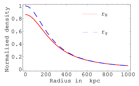
Figure 1: The modified profile $\rho_{B}(r)$ compared to the $\beta$-profile $\rho_{g}(\beta,r)$ for standard cluster values. The mean molecular weight is $\mu=0.63$. The profiles are normalized by the central gas density $\rho_{g,0}$.

Based on these profiles, the SZ-effect can be calculated. The frequency dependent intensity change of the cosmic microwave background photons (CMB) due to inverse Compton scattering off the hot intracluster electrons can be expressed as follows (Sunyaev and Zel’dovich, 1972; Rephaeli, 1995; Birkinshaw, 1999):

$$\Delta I(x)=i_{0}\,g(x)\int\limits\left(\frac{kT_{g}}{m_{e}c^{2}}\right)\sigma_{T}n_{e}\,dl,$$ (33)

where $x=\frac{h\nu}{kT}$ is the dimensionless frequency with $T$ the CMB temperature and $i_{0}=\frac{2(kT)^{3}}{(hc)^{2}}$. The function $g(x)$ defines the spectral shape of the thermal SZ-effect. The integral is the Comptonization parameter $y$ describing the cluster properties with $T_{g}$, $m_{e}$ the electron cluster temperature and electron mass, respectively. $n_{e}$ is the electron number density in the cluster and $\sigma_{T}$ the Thomson cross section. ($k$, $h$, $c$ are the Boltzmann constant, the Planck constant and the speed of light, respectively.) As we are interested in the influence of magnetic fields, we define $\alpha$ to be the ratio between the SZ-effect with the modified density $\rho_{B}(r)$ and the standard SZ-effect with $\rho_{g}(\beta,r)$. For our standard values we find:

$$\alpha:=\frac{\Delta I_{B}}{\Delta I}=\frac{\int_{0}^{r_{l}}\rho_{B}(\tilde{r})d\tilde{r}}{\int_{0}^{r_{l}}\rho_{g}(\beta,\tilde{r})d\tilde{r}}=0.92,$$ (34)

where the integration is along a line of sight through the cluster center with a limiting radius $r_{l}=1000\,kpc$. From our theoretical analysis we thus find that magnetic fields reduce the SZ-effect by $\approx\,10\%$ compared to the value one would get for an average standard cluster without magnetic fields.
Indeed, $\alpha=\alpha(B_{0},T_{g},n_{g,0},r_{l},\beta,\gamma)$ depends on several observational values. Modifying the central magnetic field strength $B_{0}$, while keeping constant the other parameters, can substantially change the ratio $\alpha$. $B_{0}\approx 1\,\mu G$ reduces the SZ-effect by less than $1\%$, whereas $B_{0}\approx 10\,\mu G$ gives $\alpha=0.85$. Similarly, a lower temperature $T_{g}=10^{7}\,K$ combined with our standard values gives $\alpha=0.84$, whereas a very hot cluster with $T_{g}=10^{8}\,K$ leads to $\alpha=0.98$. In an analogous way, $\alpha$ decreases with a smaller central gas number density $n_{g,0}$. Reducing $n_{g,0}$ by $20\%$ gives $\alpha=0.90$, instead a $20\%$ increase results in $\alpha=0.93$. A larger cluster limiting radius $r_{l}$ makes the magnetic field influence generally more important. $\alpha$ is not sensitive to little changes in the parameter $\beta$, because both $\rho_{g}(\beta,r)$ and $\rho_{B}(r)$ depend on it. Dolag et al. (2001) estimated the slope $\gamma$ for the $n_{e}$ - $B$ relation to be in the range $\gamma\in(0.5-1.0)$. $\alpha$ decreases then for lower values of $\gamma$, reaching $\alpha=0.86$ in the limiting case $\gamma=0.5$. All our results for $\alpha$, with $\gamma=0.9$, are thus still conservative estimates.

3.1.2 Observational consequences

We now switch to an observer’s point of view. The observational data of a specific cluster, like surface brightness and energy spectrum, do already contain the magnetic field effect! As argued before, fitting these data with an isothermal $\beta$-model does not correspond to the real physical picture. However, the still large error bars in the present data will not allow to discriminate between an isothermal $\beta$-fit and a fit with the profile $\rho_{B}$. This is in particular true for the value of the central cluster density, which is often affected by errors of the order of $10\%$ (see e.g. Mohr et al. (1999)). The isothermal $\beta$-profile $\rho_{g}(\beta_{Fit})$ with the parameter $\beta_{Fit}$, determined from observations, must thus be compared to $\rho_{B}$:

$$\rho_{B}=\rho_{g}(\beta)[1+h_{B}(r)]\quad\longleftrightarrow\quad\rho_{g}(\beta_{Fit}).$$ (35)

As the central cluster region is often not very well resolved in X-ray data, $\beta_{Fit}$ is usually determined using the data from the outer parts. In these regions, the magnetic field influence is very small, i.e. $h_{B}\approx 0$. In good approximation we get therefore:

$$\beta\approx\beta_{Fit}.$$ (36)

The isothermal $\beta$-model will thus overestimate the real density $\rho_{B}(r)$, because $h_{B}(r)<0$. The error will be largest in the central region where the magnetic field pressure grows fast and becomes important. The central gas density can be overestimated by $10-20\%$, as it is seen in Fig. 1. We, therefore, expect the observed SZ signal to be smaller by $\approx 10\%$ compared to the expected value as estimated from X-ray data, when the magnetic field influence has not been taken into account.
Following these arguments, we applied Eq.(11) to a well documented non-cooling flow cluster: A119, which is characterized by the presence of three extended radio galaxies. From different observations remarkably consistent values are found (Mohr et al. (1999), Dolag et al. (2001) and references therein) and the existence of a cooling flow can be excluded for all practical purposes (White et al., 1997). For an isothermal $\beta$-model, the cluster parameters are: $\beta_{Fit}=0.56$, $\gamma=0.9$, $B_{0}=7.5\,\mu G$, $T_{g}=5.92\cdot 10^{7}K$, $n_{g,0}=2.593\cdot 10^{-3}\,cm^{-3}$, $r_{c}=800\,kpc$, $r_{l}=1550\,kpc$. From our discussion above, the quoted central value $n_{g,0}$ should be overestimated. The other values are acceptable in good approximation, as explained. The results for the normalized profiles of $\rho_{B}(r)$ compared to $\rho_{g}(\beta,r)$ are shown in Fig. 2 and the calculated ratio $\alpha$ turns out to be $\alpha\approx 0.905$. As $n_{g,0}$ is overestimated, this is a conservative result and the real influence of the magnetic fields on the SZ-effect could be even a few percent larger. Reducing the central density by $10\%$ gives a ratio of $\alpha=0.895$. If magnetic fields are neglected in A119, the SZ-effect is thus overestimated by $\approx 10\%$.

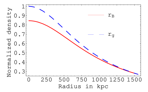
Figure 2: The modified profile $\rho_{B}(r)$ compared to the $\beta$-profile $\rho_{g}(\beta,r)$ for A119. The mean molecular weight is $\mu=0.63$. The profiles are normalized by the central gas density $\rho_{g,0}$.

3.2 Cooling flow clusters

Majumdar and Nath (2000) already studied the effect of cooling flows on the SZ distortion and the possible cosmological implications, in particular on the Hubble constant. In this section we analyse how magnetic fields, in top of their result, can influence the SZ signal. First, we discuss the solution of the Eqs.(22) and (23) with magnetic fields, and second, we give the results of our SZ calculation for the magnetic cooling flow model described in section 2.2. We distinguish the cooling flow region from the region outside $r_{cool}$. The later one is analysed following the result obtained in section 2.1.

Once the sonic radius $r_{s}$ is found from the Eqs.(28) and (29), integrating away from $r_{s}$ requires then to find nonsingular expressions for the derivatives of the differential Eqs.(22) and (23). This is a non-trivial task with the additional magnetic field contribution. Furthermore, this procedure (shooting method) requires an iterative process to match the hydrostatic boundary conditions at $r_{cool}$. If we want to separate the magnetic field influence, this gets even more complicated as we would have to match both $\rho_{B}(r_{cool})$ and $\rho_{g}(r_{cool})$ with the same cooling flow parameter $\dot{m}$. We would thus have to find possible values for $\theta_{B}(r_{s})$ and $\theta(r_{s})$ at the sonic radius - which differ by the magnetic field contribution in the Eqs.(22) and (23) - which must then lead to the required values for $\rho_{B}(r_{cool})$ and $\rho_{g}(r_{cool})$ at the cooling radius. Since these values at $r_{cool}$ are derived by the procedure described in section 2.1, they are not independent from each other neither, but related through the magnetic field strength $B(r_{cool})$. Sarazin and White (1987) were already aware of how sensitive the integration of the Eqs.(22) and (23), in the absence of magnetic fields, can be. Not only three boundary conditions ($\rho,\theta,v$) must be matched, but the possible values of them are additionally constrained by three physically motivated conditions like hydrostatic equilibrium, mass deposition rate and vanishing numerators in the Eqs.(22) and (23) for a regular remaining flow. Not surprisingly that the range of allowed boundary conditions to find a transonic flow is extremely small.
We stress that our goal is not to develop a sophisticated cooling flow model, but to get an estimate of how magnetic fields can modify the SZ-effect in a cooling flow cluster. We therefore avoid the time consuming and complicated procedure as outlined above, and start our integration with physically reasonable parameters from $r_{cool}$ towards $r_{s}$. The transition at $r_{s}$ between subsonic and supersonic is always accompanied by shocks. Moreover, this most inner part will also be under the influence of a central galaxy. Since the interplay between cooling flows, central galaxy, shocks and the SZ-effect is not clear, we do not attempt to find solutions to the Eqs.(22) and (23) inside the sonic radius $r_{s}$. We will, therefore, cut out this supersonic region for our SZ calculation. Converging cooling flows amplify the magnetic field strength enormously until the magnetic field pressure ($P_{B}$) becomes comparable to the thermal gas pressure ($P_{g}$). Our numerical studies show that this occurs typically at $\sim 10\,kpc$. The ultimate fate of the magnetic field is still a matter of debate. Field line reconnection or convective motions resulting in buoyantly rising regions might be possible answers. Furthermore, Christodoulou and Sarazin (1996) pointed out, that more realistic magnetized models can in this region not be treated correctly in spherical symmetry. Based on the above arguments we decided to stop the integration of the Eqs.(22) and (23) at the pressure equipartition radius $r_{B}(>r_{s})$, where $\frac{P_{B}}{P_{g}}\sim 1$.

We briefly discuss the input values for our results. The gravitating cluster mass $\mathcal{M}(r)$ is fixed as described in section 2.2. We assume that the cooling flow gas makes no significant contribution to the mass density of the cluster. For the region outside $r_{cool}$, a standard isothermal $\beta$-model with $\beta=\frac{2}{3}$, $T_{g}=1.9\cdot 10^{8}\,K$ and a central gas density $n_{g,0}=1.2\cdot 10^{-2}\,cm^{-3}$ is consistently adopted. We choose a magnetic field strength $B(r_{cool})\approx 1\,\mu G$, which reproduces the observed values of the order of $B_{0}\approx 50\,\mu G$ for the cluster core, as found from the cooling flow model in the Eq.(20). Assuming again $\gamma=0.9$, these values determine then with the Eq.(11) the density profiles $\rho_{g}(r)$ and $\rho_{B}(r)$ for the region outside $r_{cool}$, and define the starting values $\rho_{g}(r_{cool})$ and $\rho_{B}(r_{cool})$ for the cooling flow region. Once the mass deposition rate $\dot{m}$ is fixed, the continuity Eq.(18) completely determines the initial velocities $v_{B}(r_{cool})$ and $v(r_{cool})$ for the integration of the Eqs.(22) and (23). For these velocities at $r_{cool}$ we must require that they are of the order of a few tens of $km/s$, which corresponds to the turbulent velocity $v_{T}$. From the difference between $\rho_{B}(r_{cool})$ and $\rho_{g}(r_{cool})$, ($\rho_{B}(r_{cool})\stackrel{{\scriptstyle<}}{{\sim}}\rho_{g}(r_{cool})$), it is obvious that $|v_{B}(r_{cool})|\stackrel{{\scriptstyle>}}{{\sim}}|v(r_{cool})|$. The initial sound speed squared, $\theta_{B}(r_{cool})\equiv\theta(r_{cool})$, is directly related to $T_{B}\equiv T_{g}$. Finally, the so derived initial conditions and chosen parameters have to allow for the existence of a cooling flow: $t_{cool}\stackrel{{\scriptstyle<}}{{\sim}}t_{Hubble}$. From the above discussion it is clear that the integration with possible values from $r_{cool}$ towards $r_{s}$ is also limited by constraints, which can be summarized as follows:

$$\mathcal{M}(r)=\mathcal{M}_{B}(r),$$ (37)

$$\rho_{g}(r_{cool})=\frac{\dot{m}}{4\pi r_{cool}^{2}}\frac{1}{v(r_{cool})},\qquad|v(r_{cool})|\simeq v_{T},$$ (38)

$$\rho_{B}(r_{cool})=\frac{\dot{m}}{4\pi r_{cool}^{2}}\frac{1}{v_{B}(r_{cool})},\qquad|v_{B}(r_{cool})|\simeq v_{T},$$ (39)

$$t_{cool}=\frac{5}{2}\frac{\theta}{\rho\Lambda}\stackrel{{\scriptstyle<}}{{\sim}}t_{Hubble}\simeq 10^{10}yr.$$ (40)

These constraints have to be fulfilled with observationally reasonable values $\dot{m}$ and $B_{0}$. As a possible set of initial values and cluster parameters we have chosen: $B(r_{cool})=1\,\mu G$, $\dot{m}=-300\,M_{\odot}/yr$, $\sqrt{\theta(r_{cool})}\equiv\sqrt{\theta_{B}(r_{cool})}=1600\,km/s$, $|v(r_{cool})|=|v_{B}(r_{cool})|=15\,km/s$.

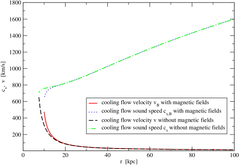
Figure 3: The influence of magnetic fields on the cooling flow velocity $|v(r)|$ and the isothermal sound speed $c_{s}(r)$ as a function of radius. The mass deposition rate is $\dot{m}=-300\,M_{\odot}yr^{-1}$, $r_{cool}=100\,kpc$ and $B(r_{cool})=1\mu G$. The initial conditions for the integration are: $\sqrt{\theta(r_{cool})}=\sqrt{\theta_{B}(r_{cool})}=1600\,km/s$ and $|v(r_{cool})|=|v_{B}(r_{cool})|=15\,km/s$.

Fig.3 shows how the cooling flow dynamics are influenced by magnetic fields. The integration for the profiles with magnetic fields is stopped at the pressure equipartition radius $r_{B}$, whereas the profiles in absence of magnetic fields are stopped close to the sonic radius $r_{s}$ where the Mach number is $M\approx 0.9$.

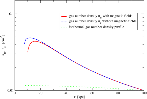
Figure 4: The influence of magnetic fields on the cooling flow gas number density. Parameters and initial conditions as adopted in Fig.3.

Fig.4 and Fig.5 give the corresponding gas number density and temperature profiles for the cooling flow region. Since the magnetic field strength at $r_{cool}$ is very weak, but the cluster temperature high, the difference between $\rho_{g}(r_{cool})$ and $\rho_{B}(r_{cool})$ is completely negligible, as it results from Eq.(11). Therefore, the initial velocities $|v(r_{cool})|$ and $|v_{B}(r_{cool})|$ can be set equal for all practical purposes. The influence of the magnetic fields on the SZ-effect is thus entirely determined by the cooling flow region.
Similarly to Eq.(34), we define a ratio $\alpha_{CF}$ for the cooling flow $(CF)$ region. For our parameters we find:

$$\alpha_{CF}:=\frac{\Delta I_{B,CF}}{\Delta I_{CF}}=\frac{\int_{r_{B}}^{r_{cool}}\rho_{B}(\tilde{r})T_{B}(\tilde{r})d\tilde{r}}{\int_{r_{B}}^{r_{cool}}\rho_{g}(\tilde{r})T_{g}(\tilde{r})d\tilde{r}}=0.98,$$ (41)

where we cut out the most central part of the cluster and the lower integration limit is taken to be the pressure equipartition radius $r_{B}=10\,kpc$. If the above ratio is completed with the SZ contribution from the isothermal region outside $r_{cool}$, ($T_{g}\int_{r_{cool}}^{r_{l}}\rho_{iso}(\tilde{r})d\tilde{r},$ with $\rho_{iso}$ an isothermal $\beta$-model and $r_{l}=1000\,kpc$), one finds $\alpha_{CF}\approx 0.99$. The presence of magnetic fields reduces thus only slightly the cooling flow correction to the SZ-effect. When calculating the ratio $\alpha_{B}$ between the magnetic field influenced profiles and the standard isothermal profiles, we find instead:

$$\alpha_{B}:=\frac{\Delta I_{B,CF}}{\Delta I}=\frac{\int_{r_{B}}^{r_{cool}}\rho_{B}(\tilde{r})T_{B}(\tilde{r})d\tilde{r}+T_{g}\int_{r_{cool}}^{r_{l}}\rho_{iso}(\tilde{r})d\tilde{r}}{T_{g}\int_{r_{B}}^{r_{l}}\rho_{iso}(\tilde{r})d\tilde{r}}=1.01,$$ (42)

compared to $1.02$, which we get without taking into account the magnetic field in the cooling flow. This is not surprising because of the weakness of the initial magnetic field strength at $r_{cool}$, which leads to practically identical initial conditions. The magnetic field strength becomes only important towards the very center and there it then almost compensates the small cooling flow effect. For the chosen parameters, magnetic field and even cooling flow do not modify much the SZ-effect.
Nevertheless, our numerical investigations showed that for a higher magnetic field strength, $B(r_{cool})\approx 6\,\mu G$, and a higher temperature, $T_{g}\approx 5\cdot 10^{8}\,K$, the ratio in Eq.(41) can reach $\alpha_{CF}=0.94$. Moreover, at variance with the above discussed example, a higher magnetic field strength at $r_{cool}$ leads also to a sizeable lower gas density, as compared to the case without magnetic field, in the region outside $r_{cool}$. This fact, as discussed in Section 3.1.1, modifies accordingly the contribution to the SZ-effect coming from the integration outside $r_{cool}$. For such cooling flow parameters, Majumdar and Nath (2000) expect an overestimation of the standard SZ-effect by $\sim 10\%$, due to the presence of a non-magnetized cooling flow. We instead find that this overestimation gets reduced to $5-8\%$ when the (higher) magnetic field is taken into account. Finally we note that our results are conservative estimates since we always cut out the most central part of the cluster.

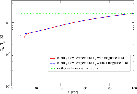
Figure 5: The influence of magnetic fields on the cooling flow temperature. Parameters and initial conditions as adopted in Fig.3.

4 Conclusions

In a phenomenological approach we added the magnetic field pressure to the gas pressure and for clusters without cooling flows we derived in a perturbative procedure a new gas density profile. This can be related to a standard $\beta$-profile and a function, which takes into account the radius dependent magnetic field strength, which is assumed to be correlated to the electron density. For reasonable cluster parameters we find that magnetic fields reduce the standard SZ signal by $\sim 10\%$. Indeed, a reduction of up to $\sim 15\%$ seems possible. Our perturbative approach based on the equal mass assumption, $\mathcal{M}_{B}(r)=\mathcal{M}(r)$, turns out to be well justified by this order of magnitude correction: The corresponding decrease in the gas density is $\leq 10-15\%$ and, therefore, the change in the dark matter dominated total cluster mass profile is less than $1\%$. The simplifying assumption of an isothermal temperature is adequate, because the interplay between temperature and a variable magnetic field strength is not yet very clear (Dolag et al., 2001).
Furthermore, our considerations showed that the central cluster gas density is probably overestimated by $10-20\%$ when fitted with a standard $\beta$-model. Better data in future might reveal the need for a modified $\beta$-profile as discussed here.
Other possible causes of deviations from the (standard) $\beta$-model have been discussed in the literature in the context of the determination of the Hubble constant (Birkinshaw et al. (1991); Inagaki et al. (1995) and references therein). Generally, the finite extension of a cluster (already adopted in our calculation) lowers the SZ signal by $5-10\%$ compared to the case of an infinite isothermal $\beta$-model, and requires then a larger core radius $r_{c}$ in the $\beta$-model. Other departures from the standard $\beta$-model include asphericity and small-scale clumping. The most extreme variation of geometry of the original spherical model is obtained if the unique axis of the prolate ($Z>1$) or oblate ($Z<1$) gas distribution is oriented along the line of sight. The SZ signal scales then with the factor $Z$, which is the ratio of the length of the unique axis to the major or minor axis, respectively. Typically, $0.5<Z<2$, and asphericity introduces thus a variation of a factor $\sim 2$ in the core radius $r_{c}$. Whereas this effect will be averaged out in a large enough cluster sample, all cluster atmospheres will be clumpy to some degree. This might result in an overestimation of the standard SZ signal at the percentage level, but current simulations are limited in resolution and clumpiness might be more important. Whereas all these effects modify the parameters of the standard $\beta$-model, the inclusion of magnetic fields requires an extended $\beta$-profile, which takes explicitly into account the magnetic field strength. Unfortunately, in an integrated SZ measurement all the effects will sum up and they can hardly be separated. Precise future X-ray data might then help to reveal the inner cluster structure.

For the cooling flow clusters, following the treatment by Soker and Sarazin (1990), we generalized the equations for the sound speed and infall velocity derived by Mathews and Bregman (1978) such as to include also a magnetic field. For typical initial magnetic field values at $r_{cool}$, $P_{B}/P_{g}\sim 10^{-4}$, we find an equipartition radius $r_{B}\sim 10\,kpc$ and we derive profiles which are in agreement with Soker and Sarazin. Our somewhat larger sonic radius $r_{s}\sim 5\,kpc$ - though not irrealistic as it was found by Sulkanen et al. (1989), who derived sonic radii of $\sim 10-20\,kpc$ for plausible cluster and cooling flow parameters - results probably from different initial conditions. As the integration for the equations of sound speed and infall velocity is very delicate or even impossible for any arbitrary combination of parameters, our results can not immediately be generalized. Current discussions about the magnetic field model in the cooling flow region limit further our conclusions. Nevertheless, it turns out that the gas density in the cooling flow gets somewhat smaller in the presence of magnetic fields as compared to the case without. This translates then into a weaker influence of the order of some percent of the magnetized cooling flow on the SZ-effect. In special cases magnetic fields might almost compensate the cooling flow correction to the SZ-effect.
Indeed, a precise calculation would require more sophisticated models which are adapted to the specific cluster parameters. For all these reasons, cooling flow clusters do not seem to be ideal targets for SZ observations.

Acknowledgments

This work was supported by the Swiss National Science Foundation. Part of the work of D.P. has been conducted under the auspices of the Dr Tomalla Foundation.

References

- Birkinshaw et al. (1991) Birkinshaw, M., Hughes, J.P., Arnaud, K.A., 1991. ApJ 379, 466
- Birkinshaw (1999) Birkinshaw, M., 1999. Phys. Rep. 310, 97
- Blasi (2000) Blasi, P., 2000. ApJ 532, 9
- Blasi et al. (2000) Blasi, P., Olinto, A.V., Stebbins, A., 2000. ApJ 535, L71
- Challinor and Lasenby (1998) Challinor, A., Lasenby, A., 1998. ApJ 499, 1
- Christodoulou and Sarazin (1996) Christodoulou, D.M., Sarazin, C.L., 1996. ApJ 463, 80
- Clarke et al. (1999) Clarke, T.E., Kronberg, Ph.P., Böhringer, H. in: Proceedings of the Workshop: “Diffuse Thermal and Relativistic Plasma in Galaxy Cluster”, 1999, eds. H. Böhringer, L. Feretti & P.Schuecker, MPE Report 271, 82
- Clarke et al. (2001) Clarke, T.E., Kronberg, P.P., Böhringer, H. 2001. ApJ 547, L111
- Cooray and Chen (2001) Cooray, A., Chen, X., 2002. ApJ 573, 43
- Dolag et al. (2001) Dolag, K., Schindler, S., Govoni, F., Feretti, L., 2001. AA 378, 777
- Eilek and Owen (2001) Eilek, J.A., Owen, F.N., 2001. ApJ 567, 202
- Ensslin et al. (1999) Ensslin, T.A., Lieu, R., Biermann, P.L., 1999. AA 344, 409
- Fabian et al. (1991) Fabian, A.C., Nulsen, P., Canizares, C., 1991. AA Rev. 2, 191
- Fabian (1994) Fabian, A.C., 1994. Ann. Rev. Astrophys. 32, 277
- Fusco-Femiano et al. (1999) Fusco-Femiano, R., dal Fiume, D., Feretti, L., Giovannini, G., Grandi, P., Matt, G., Molendi, S., Santangelo, A., 1999. ApJ 513, L21
- Feretti et al. (1995) Feretti, L., Dallacasa, D., Giovannini, G., Tagliani, A., 1995. AA 302, 680
- Ge and Owen (1993) Ge, J.P., Owen, F.N., 1993. AJ 105, 778
- Gonçalves and Friaça (1999) Gonçalves, D.R., Friaça, A.C., 1999. MNRAS 309, 651
- Giovannini et al. (1999) Giovannini, G., Tordi, M., Feretti, L., 1999. New Astronomy 4, 141
- Giovannini and Feretti (2000) Giovannini, G., Feretti, L., 2000. New Astronomy 5, 335
- Gitti et al. (2002) Gitti, M., Brunetti, G., Setti, G., 2002. AA 386, 456
- Govoni et al. (1999) Govoni, F., Dallacasa, D., Feretti, L., Giovannini, G., Taylor, G.B. in: Proceedings of the Workshop:“Diffuse Thermal and Relativistic Plasma in Galaxy Cluster”, 1999, eds. H. Böhringer, L. Feretti & P.Schuecker, MPE Report 271, 87
- Gruber and Rephaeli (2002) Gruber, D.E., Rephaeli, Y., 2002. ApJ 565, 877
- Inagaki et al. (1995) Inagaki, Y., Suginohara, T., Suto, Y., 1995. PASJ 47, 411
- Itoh et al. (1998) Itoh, N., Kohyama, Y., Nozawa, S., 1998. ApJ 502, 71
- Loeb and Mao (1994) Loeb, A., Mao, S., 1994. ApJ 435, L109
- Jaffe (1980) Jaffe, W., 1980. ApJ 241, 925
- Kaastra et al. (1999) Kaastra, J.S., Lieu, R., Mittaz, J.P.D., Bleeker, J.A.M., Mewe, R., Colafrancesco, S., Lockman, F.J., 1999. ApJ 519, L119
- King (1966) King, I.R., 1966. Astron.J. 71, 64
- Majumdar and Nath (2000) Majumdar, S., Nath, B., 2000. ApJ 542, 597
- Majumdar et al. (2001) Majumdar, S., Nath, B., Chiba, M., 2001. MNRAS 324, 537
- Mathews and Bregman (1978) Mathews, W.G., Bregman, J.N., 1978. ApJ 224, 308
- Mohr et al. (1999) Mohr, J.J., Mathiesen, B., Evrard, A.E., 1999. ApJ 517, 627
- Molendi et al. (2000) Molendi, S., De Grandi, S., Fusco-Femiano, R., 2000. ApJ 534, L43
- Puy et al. (2000) Puy, D., Grenacher, L., Jetzer, Ph., Signore, M., 2000. AA 363, 415
- Raymond et al. (1976) Raymond, J.C., Cox, D.P., and Smith, B.W., 1976. ApJ 204, 290
- Rephaeli (1995) Rephaeli, Y., 1995. Annu. Rev. Astron. Astrophys. 33, 541
- Rephaeli et al. (1999) Rephaeli, Y., Gruber, D., Blanco, P., 1999. ApJ 511, L21
- Sandoval-Villalbazo and Maartens (2002) Sandoval-Villalbazo, A., Maartens, R., 2001. astro-ph/0105323
- Sarazin (1988) Sarazin, C., 1988. in: X-ray emission from clusters of galaxies, Cam. Uni. Press
- Sarazin and White (1987) Sarazin, C., White, III R.E., 1987. ApJ 320, 32
- Schlickeiser (1991) Schlickeiser, R., 1991. AA 248 , L23
- Schmutzler and Tscharnuter (1993) Schmutzler, T., Tscharnuter, W.M., 1993. AA 273, 318
- Shimon and Rephaeli (2002) Shimon, M., Rephaeli, Y., 2002. astro-ph/0204355
- Soker and Sarazin (1990) Soker, N., Sarazin, C.L., 1990. ApJ 348, 73
- Sulkanen et al. (1989) Sulkanen, M.E., Burns, J.O., Norman, M.L., 1989. ApJ 344, 604
- Sunyaev and Zel’dovich (1972) Sunyaev, R.A., Zel’dovich, Ya.B., 1972. Comm. Astrophys. Space Phys. 4, 173
- Taylor and Perley (1993) Taylor, G.B., Perley, R.A., 1993. ApJ 416, 554
- Taylor et al. (1999) Taylor, G.B., Allen, S.W., Fabian, A.C., in: Proceedings of the Workshop: “Diffuse Thermal and Relativistic Plasma in Galaxy Cluster”, 1999, eds. H. Böhringer, L. Feretti & P.Schuecker, MPE Report 271,77
- Taylor et al. (2001) Taylor, G.B., Fabian, A.C., Allen, S.W., 2001 astro-ph/0109337
- Tribble (1991) Tribble, P.C., 1991. MNRAS 250, 726
- Tribble (1993) Tribble, P.C., 1993. MNRAS 263, 31
- White et al. (1997) White, D., Jones, C., Forman, W., 1997. MNRAS 292, 419
- White and Sarazin (1987a) White, III R.E., Sarazin, C., 1987a. ApJ 318, 612
- White and Sarazin (1987b) White, III R.E., Sarazin, C., 1987b. ApJ 318, 629