Effects of a Soft X-ray Background on Structure Formation at High Redshift

Abstract

We use three dimensional hydrodynamic simulations to investigate the effects of a soft X-ray background, that could have been produced by an early generation of mini-quasars, on the subsequent cooling and collapse of high redshift pregalactic clouds. The simulations use an Eulerian adaptive mesh refinement technique with initial conditions drawn from a flat $\Lambda$-dominated cold dark matter model cosmology to follow the nonequilibrium chemistry of nine chemical species in the presence of both a soft ultraviolet Lyman-Werner H₂ photodissociating flux of strength $F_{LW}=10^{-21}$  erg s^-1 cm^-2 Hz^-1 and soft X-ray background extending to $7.2$ keV including the ionization and heating effects due to secondary electrons. Although we vary the normalization of the X-ray background by two orders of magnitude, the positive feedback effect of the X-rays on cooling and collapse of the pregalactic cloud expected due to the increased electron fraction is quite mild, only weakly affecting the mass threshold for collapse and the fraction of gas within the cloud that is able to cool, condense and become available for star formation. Inside most of the cloud we find that H₂ is in photodissociation equilibrium with the soft UV flux. The net buildup of the electron density needed to enhance H₂ formation occurs too slowly compared to the H₂ photodissociation and dynamical timescales within the cloud to overcome the negative impact of the soft UV photodissociating flux on cloud collapse. However, we find that even in the most extreme cases the first objects to form do rely on molecular hydrogen as coolant and stress that our results do not justify the neglect of these objects in models of galaxy formation. Outside the cloud we find the dominant effect of a sufficiently strong X-ray background is to heat and partially ionize the inter-galactic medium, in qualitative agreement with previous studies.

1 Introduction

One of the most important questions in current cosmology is to understand how the cosmological dark ages ended by identifying the nature of the first luminous sources and determining their impact on subsequent structure formation and the reionization of the universe. Recent observations are beginning to constrain the epoch of reionization and give modest information about possible first sources. Observations of metals throughout even low column density Ly$\alpha\$lines (Ellison et al. 1999, 2000; Schaye et al. 2000) suggest the need for an early population of stars to pre-enrich the inter-galactic medium (IGM). Observed spectra of high redshift quasars such as SDSS 1030+0524 (Fan et al. 2001) at $z=6.28$ and Ly$\alpha\$emitters at these redshifts (e.g. Hu et al. 2002) start to constrain the overlap stage of hydrogen reionization. Observations of patchiness in the HeII optical depth in the Lyman alpha forest at $z\sim 3$ (Reimers et al. 1997) might signal a recent period of helium reionization. Multi-wavelength observations planned in the near future hope to study the reionization epoch in detail. Direct imaging of quasars and star clusters at $z>10$ may be possible using the Next Generation Space Telescope (Haiman & Loeb 1999, Barkana & Loeb 2000). Emission measurements in the 21 cm line using LOFAR and the Square Kilometer Array could identify the first epoch of massive star formation (Tozzi et al. 2000). Searches for polarization effects and secondary anisotropies in the Cosmic Microwave Background induced by scattering off the increased electron fraction produced during reionization are planned by Planck and the next generation of millimeter telescopes such as ALMA.

In order to correctly interpret the findings of these observations, we need to understand the predictions of the current cosmological structure formation paradigm. The initial stages of collapse of structure at high redshift in cold dark matter cosmologies have been well studied analytically and numerically (see, for example, the excellent review by Barkana & Loeb 2001 and references therein). Structure forms from small density perturbations via gravitational instability where smaller clumps merge to form larger clumps within and at the intersections of filaments. By redshifts $30\la z\la 20$ pregalactic clouds with masses (virial temperatures) $M\sim 10^{5}$ - $10^{6}\,M_{\odot}$ ( $T_{vir}\sim 1000$  K ) have formed sufficient molecular hydrogen to begin to cool reducing pressure support in their central regions and allowing their cores to collapse to high density (Haiman, Thoul & Loeb 1996; Tegmark et al. 1997; Omukai & Nishi 1998; Abel et al. 1998; Fuller & Couchman 2000). However, it is only recently that 3-D numerical simulations have achieved sufficient resolution to follow this collapse reliably from cosmological initial conditions to the extremely high densities and stellar spatial scales expected for the first luminous sources (Abel, Bryan, & Norman 2000, 2001). These and related studies (e.g. Bromm, Coppi & Larson 2001; Nakamura & Umemura 2001) show that the final stages of collapse are slow (quasi-static) and that fragmentation in the primordial, metal-free gas is difficult. Thus the first sources were most probably massive stars. This has led to renewed interest in the evolutionary properties of such metal-free, massive stars (Fryer, Woosley & Heger 2001; Schneider et al. 2001; Oh 2001; Oh et al. 2001). However, the micro-galaxies ($\ga 10^{6}M_{\odot}\approx 10^{-6}$ times the mass of the Milky Way) which host the first stars collapse over a large redshift interval. At the same time in different regions of space also rarer but much larger objects are forming whose integrated emitted light cannot be reliably predicted nor constrained strongly from existing observations. Consequently, the radiation spectrum from the first luminous sources is uncertain.

Clearly, a background of soft ultraviolet (UV) radiation is expected from the first stars. The neutral primordial gas remains optically thin to soft UV photons below the hydrogen ionization edge until the gas collapses to high density. In particular photons in the Lyman-Werner bands ($11.2\,{\rm eV}\,<E_{\gamma}<13.6$ eV) can travel large distances and readily photodissociate the fragile H₂ coolant in their own and neighboring clouds via the two-step Solomon process. Such a soft UV background alone is expected to suppress the subsequent collapse of low mass clouds ($T_{vir}<10^{4}$  K ) that require H₂ to cool (Dekel & Rees 1987; Haiman, Rees & Loeb 1997; Omukai & Nishi 1999; Ciardi et al. 2000; Haiman, Abel & Rees 2000; Glover & Brand 2001; Machacek, Bryan & Abel 2001; Oh & Haiman 2001). In Machacek, Bryan & Abel (2001, hereafter referred to as MBAI) we used fully 3-dimensional AMR simulations in the optically thin approximation starting from cosmological initial conditions in a $\Lambda$CDM cosmology to follow the evolution and collapse of pregalactic clouds in the presence of varying levels of soft UV flux, $0\leq F_{LW}\leq 10^{-21}$  erg s^-1 cm^-2 Hz^-1 . We confirmed that the presence of a Lyman-Werner flux $F_{LW}$ delays the onset of collapse until the pregalactic clouds evolve to larger masses and found a fitting formula for the mass threshold for collapse given the mean flux in the Lyman-Werner bands. In MBAI we also investigated what fraction of gas could cool and condense and thus become available for star formation, an important input parameter for semi-analytical models of galaxy formation, stellar feedback and its impact on the process of reionization (Ciardi et al. 2000, Ciardi, Ferrara, & Abel 2000, Madau, Ferrara, & Rees 2001). We found that the fraction of gas that could cool and become dense in metal-free pregalactic clouds in our simulations depended primarily on two numbers, the flux of soft UV radiation and the mass of the cloud, and that once above the collapse mass threshold determined by the level of photodissociating flux, the fraction of cold, dense gas available for star formation in these early structures increased logarithmically with the cloud’s mass.

If early luminous sources include a population of mini-quasars or other X-ray emitting sources such as X-ray binaries they will produce a background radiation field of soft X-rays with energies above the Lyman limit ($\ga 1$ keV). It has been suggested (Haiman, Rees & Loeb 1996; Haiman, Abel & Rees 2000; Oh 2001; Ricotti, Gnedin & Shull 2001) that the increased electron fraction produced by the ionizing photons would promote the formation of H₂ thereby undoing the negative feedback effect of the soft, Lyman-Werner UV flux on the collapse of low mass pregalactic clouds. Haiman, Rees & Loeb (1996) found that the formation rate of H₂ could be enhanced in a dense ($n_{H}\ga 1$ cm^-3), stationary, homogeneous gas cloud of primordial composition irradiated by an external, uniform power-law background flux with photon energies $\la 40$ keV. Their calculations assumed chemical equilibrium for the species. They used Lepp & Shull (1983) cooling functions for molecular hydrogen and mimicked radiative transfer effects by assuming a mean absorbing column density of $10^{22}$  cm^-2 . Haiman, Abel & Rees (2000) again considered H₂ formation in a static, isolated primordial cloud in the presence of a power-law radiation flux extending to $10$ keV. However, they adopted the more realistic profile of a truncated isothermal sphere at its virial temperature and followed the time evolution of nine chemical species. They concluded that in the cores of these objects the negative effect of the photodissociating flux on collapse is erased if as little as $10\%$ of the radiation field is from mini-quasars with energies extending into the soft X-ray band. In two recent papers, Ricotti et al. (2002a, 2002b) have also examined the effect of radiative feedback on cooling in low-mass halos and find that high-energy photons can have a positive net effect on the star formation rate.

In this paper we extend the results of our fully 3-D Eulerian AMR simulations of the formation and collapse of primordial pregalactic structure in the presence of a soft Lyman-Werner UV background (MBAI) to include the contribution of X-rays with energies extending to $7.2$ keV. This work, as in MBAI, improves upon earlier studies by following the time evolution of a collection of collapsing protogalaxies evolving together in a $1$ Mpc³ (comoving) simulation volume from cosmological initial conditions drawn from a flat $\Lambda$CDM model. Thus it treats consistently the density evolution of the cloud and includes the effects of gravitational tidal forces and merging that also impact cooling and collapse. We develop statistics on the amount of gas that can cool due to molecular hydrogen and the fraction of gas that is cold and dense enough to be available for star formation in these objects when exposed to both a soft H₂ photodissociating flux and various levels of X-rays. We also use the more recent Galli & Palla (1998) H₂ cooling functions in this work and fitting functions for the energy deposition from high energy electrons from Shull & Van Steenberg (1985) that take into account the primordial composition of the gas.

This paper is organized in the following way: In §2 we review the set-up of our simulations with particular emphasis on our treatment of photoionization and the effects of secondary electrons induced by the X-ray background. In §3 we discuss our peak identification method and the general characteristics of our simulated data set of pregalactic clouds. In §4 we investigate how varying the intensity of the X-ray background affects the amount of gas that can cool and condense, thus becoming available for star formation, in the presence of both an H₂ photodissociating flux $F_{LW}$ and ionizing X-ray background. In §5 we use radial profiles of cloud properties to elucidate the effects of the competing physical processes important to cooling and collapse. We summarize our results in §6.

2 Simulations

We use the same simulation procedure, cosmology, initial conditions, and simulation volume as in our previous work (MBAI) so that we can directly compare the results of both studies. We summarize that technique here for completeness, but refer the reader to MBAI for a more detailed discussion. We used a flat, low matter density $\Lambda$CDM model for the simulations whose parameters were chosen to give good consistency with observation. Specifically, $\Omega_{0}=0.4$, $\Omega_{b}=0.05$, $\Omega_{\Lambda}=0.6$, $h=0.65$, $\sigma_{8}=0.8$, and $n=1$ where $\Omega_{0}$, $\Omega_{b}$, and $\Omega_{\Lambda}$ are the fraction of the critical energy density carried in nonrelativistic matter, baryons, and vacuum energy, respectively, $h$ is the dimensionless Hubble parameter in units of $100$  km s^-1 Mpc^-1 , $\sigma_{8}$ is the density fluctuation normalization in a sphere of radius $8h^{-1}$ Mpc, and $n$ is the slope of the primordial density perturbation power spectrum.

Our data set consists of results from six simulations starting from identical cosmological initial conditions on the density fields derived from the $F_{LW}=10^{-21}$ erg s^-1 cm^-2 Hz^-1 simulation in MBAI. That simulation was initialized at $z=99$ with density perturbations generated for the above $\Lambda$CDM model using the Eisenstein & Hu (1998) transfer functions. The density perturbations were evolved in a $1$ Mpc³ comoving simulation volume using a fully 3-dimensional Eulerian adaptive mesh refinement (AMR) simulation code (Bryan 1999; Bryan & Norman 1997, 1999) that forms an adaptive hierarchy of rectangular grid patches at various levels of resolution where each grid patch covers some region within its parent grid needing additional refinement and may itself become a parent grid to an even higher resolution child grid. Once an active region of structure formation was identified in the simulation box, it was surrounded by multiple static refinement levels to achieve a mass resolution within that region of $4.78M_{\odot}$ and $38.25M_{\odot}$ in the initial conditions for the gas and dark matter, respectively. The region of interest was allowed to dynamically refine further to a total of $14$ levels on a $64^{3}$ top grid resulting in a maximum dynamic range of $10^{6}$ and comoving spatial resolution at maximum refinement of $0.95$ pc (corresponding to a physical spatial resolution at $z=19$ of $0.05$ pc). As in MBAI we call a peak “collapsed” when it reaches maximal refinement. Once a peak has maximally refined we can not follow the evolution of its innermost region further. At this point we introduced artificial pressure support within the inner $1-2$ pc of the core to stabilize it against further collapse (and prevent the onset of numerical instability), so that we could continue to follow the evolution of structure elsewhere. Since most of the cooling occurs outside of the collapsed H₂ core, this should not affect the determination of the cooled gas fractions presented in §4.

We model the H₂ photodissociating Lyman-Werner flux in the same way as in MBAI by assuming a constant flux $F_{LW}$ throughout the simulation with mean photon energy $12.86$ eV, thus neglecting its time-dependent turn-on and buildup. H₂ is photodissociated by the two-step Solomon process

$$H_{2}+\gamma\rightarrow H_{2}^{*}\rightarrow H+H,$$ (1)

with rate coefficient given by (Abel, et al. 1997)

$$k_{diss}=1.1\times 10^{8}F_{LW}\,\hbox{\rm s${}^{-1}$}.$$ (2)

where $H_{2}^{*}$ is any of the $76$ Lyman-Werner resonances in the $11.18$–$13.6$ eV energy range. We work in the optically thin approximation and argue that the effect of self-shielding of the UV flux by the collapsing cores will be small so that we can neglect it. We also neglect the photodetachment of $H^{-}$ that might hinder the buildup of H₂ since $H^{-}$ is needed to catalyze the formation of molecular hydrogen. However, at the internal cloud temperatures and densities considered here we expect $H^{-}$ photodetachment to be suppressed by at least two orders of magnitude relative to H₂ formation. We refer the reader to MBAI, Section 6, for a detailed discussion of these neglected processes.

In three of our simulations we turn on an additional ionizing X-ray radiation field at $z=30$. This redshift was chosen because it was the earliest redshift found in MBAI at which sources reached maximal refinement in the absence of any radiation field. For ease of comparison we model the X-ray field $F_{x}$ in the same way as Haiman, Abel & Rees (2000) using an absorbed power law spectral form given by

$$F_{x}=\epsilon_{x}F_{LW}\biggl{(}\frac{\nu}{12.86}\biggr{)}^{-\alpha}{\rm exp}[-10^{22}(\sigma_{\hbox{H~{}$\rm\scriptstyle I\ $}}+0.08\sigma_{\hbox{He~{}$\rm\scriptstyle I\ $}})]$$ (3)

with $\alpha=1$, $F_{LW}=10^{-21}$  erg s^-1 cm^-2 Hz^-1 , corresponding roughly to a spectral intensity $J_{21}=0.1$ (Haiman, Abel & Rees, 2000), and photon energies extending to $7.2$ keV. The exponential factor was chosen to approximate the absorption of photons with energies above $13.6$ eV by the neutral IGM (and thus mimic the effects of radiative transfer on average) by assuming a constant absorbing column density of $10^{22}$  cm^-2 for hydrogen, a helium column density reduced by a factor $0.08$, representing the ratio of helium to hydrogen number densities, and ionization cross sections $\sigma_{HI}$ and $\sigma_{HeI}$ for H $\rm\scriptstyle I\$and He $\rm\scriptstyle I\$. The parameter $\epsilon_{x}$ sets the relative contributions of the X-ray and soft UV component to the background radiation field. We consider four X-ray normalizations, $\epsilon_{x}=0$, $0.1$, $1$, and $10$, where $\epsilon_{x}=0$ denotes cases with only the soft Lyman-Werner flux.

Our simulations follow the nonequilibrium, time-dependent evolution of nine chemical species (H, H⁺, He, He⁺, He⁺⁺, e^-, H₂ , H${}^{+}_{2}$, H^-) using the algorithm of Anninos, et al. (1997) initialized with post-recombination abundances (Anninos & Norman 1996). The rate coefficients for the reaction network for these species are primarily those described in MBAI. We have in this work, however, updated the H₂ cooling function to that given in Galli & Palla (1998). As a check on how this affects our results, we simulate the $\epsilon_{x}=0$ (soft UV flux only) case using both the Lepp & Shull (1983) cooling function from previous work and the Galli & Palla (1998) cooling function used for the X-ray simulations here. As shown in Figure 1, there is statistically little difference between the characteristics of the population of pregalactic objects produced using the Galli & Palla (1998) H₂ cooling function in the presence of a Lyman-Werner UV flux $F_{LW}=10^{-21}$  erg s^-1 cm^-2 Hz^-1 and those produced in an identical simulation using the cooling function of Lepp & Shull (1983). Cooling is somewhat more efficient using the Galli & Palla cooling function in the most massive peaks ($M\ga 2\times 10^{6}M_{\odot}$) in our sample, resulting in a slight drop in mean temperature for these clouds and a modest increase in the fraction of gas that can cool. (See also Table 1 and §4). Although the dependence is weak, we present both of these cases, $\epsilon_{x}=0$ gp using the Galli & Palla cooling function and $\epsilon_{x}=0$ ls using the Lepp & Shull cooling function, as a measure of the sensitivity of our results to the parameterization of the cooling chemistry. A sixth simulation ($\epsilon_{x}=0$,$F_{LW}=0$) evolves the same $z=30$ initial conditions forward using Galli & Palla cooling functions in the absence of any external radiation field to test whether the X-rays can completely overcome the effects of the photodissociating flux turning a negative feedback effect into a net positive one.

The dominant reaction chain for the production of the H₂ coolant,

$$H+e^{-}\rightarrow H^{-}+\gamma$$ (4)

$$H+H^{-}\rightarrow H_{2}+e^{-},$$ (5)

is critically dependent on the electron abundance in the cloud. When X-rays are present, the electron fraction increases both because of the primary ionization of H $\rm\scriptstyle I\$, He $\rm\scriptstyle I\$, and He $\rm\scriptstyle II\$by the X-ray photon and because of the production of secondary electrons through subsequent interactions of the primary high energy electron with the gas. We follow the time evolution of the electron fraction including the effects of the X-ray secondary electrons on subsequent ionizations and heating of the gas. In general the fractions of the primary electron energy deposited as secondary ionizations and as heat depend on the energy of the primary electron. However, for primary electron energies much greater than $100$ eV they rapidly approach a constant locus. Since most of the X-ray energy input comes from high energy photons, we use the analytic fits of Shull & Van Steenberg (1985) to these asymptotic forms. Thus the fractions of primary electron energy, $f_{1}$ and $f_{2}$, available for further ionizations of H $\rm\scriptstyle I\$and He $\rm\scriptstyle I\$are

$$f_{1}=0.3908(1-x^{0.4092})^{1.7592}$$ (6)

for H $\rm\scriptstyle I\$and

$$f_{2}=0.0554(1-x^{0.4614})^{1.6660}$$ (7)

for He $\rm\scriptstyle I\$where $x$ is the ionization fraction, $x=n_{HII}/(n_{HI}+n_{HII})$. The rate coefficients for HI and HeI ionization, including the effects of the secondary electrons, are then given by

$$\begin{split}k_{24}=&\int_{\nu_{HI}}^{\infty}\frac{F_{x}\sigma_{HI}}{h_{P}\nu}\,d\nu+f_{1}\biggl{(}\int^{\infty}_{\nu_{HI}}\frac{F_{x}\sigma_{HI}}{h_{P}\nu}\bigl{(}\frac{\nu-\nu_{HI}}{\nu_{HI}}\bigr{)}\,d\nu\\ &+\frac{n_{HeI}}{n_{HI}}\int^{\infty}_{\nu_{HeI}}\frac{F_{x}\sigma_{HeI}}{h_{P}\nu}\bigl{(}\frac{\nu-\nu_{HeI}}{\nu_{HI}}\bigr{)}\,d\nu\biggr{)}\end{split}$$ (8)

for H $\rm\scriptstyle I\$ionization and

$$\begin{split}k_{26}&=\int_{\nu_{HeI}}^{\infty}\frac{F_{x}\sigma_{HeI}}{h_{P}\nu}\,d\nu+f_{2}\biggl{(}\frac{n_{HI}}{n_{HeI}}\int^{\infty}_{\nu_{HI}}\frac{F_{x}\sigma_{HI}}{h_{P}\nu}\bigl{(}\frac{\nu-\nu_{HI}}{\nu_{HeI}}\bigr{)}\,d\nu\\ &+\int^{\infty}_{\nu_{HeI}}\frac{F_{x}\sigma_{HeI}}{h_{P}\nu}\bigl{(}\frac{\nu-\nu_{HeI}}{\nu_{HeI}}\bigr{)}\,d\nu\biggr{)}\end{split}$$ (9)

for He $\rm\scriptstyle I\$ionization with $\sigma_{HI}$ ($\nu_{HI}$) and $\sigma_{HeI}$($\nu_{HeI}$) the ionization cross sections (threshold frequencies) for H $\rm\scriptstyle I\$and He $\rm\scriptstyle I\$, $n_{HI}$ and $n_{HeI}$ the H $\rm\scriptstyle I\$and He $\rm\scriptstyle I\$number densities, $F_{x}$ the ionizing X-ray radiation field, $h_{P}$ Planck’s constant, and $h_{P}\nu$ the ionizing photon’s energy. In practice the contribution of He $\rm\scriptstyle II\$to the above processes is negligible and so we drop it. The fraction $f_{3}$ of the primary electron energy deposited as heat in the gas is (Shull & Van Steenberg, 1985)

$$f_{3}=0.9971(1-(1-x^{0.2663})^{1.3163}).$$ (10)

We self-consistently evolve the ionization fraction $x$ throughout the simulation using it to evaluate the $x$-dependent rate and heating functions (Equations 8 - 10) at each time step after turn-on of the ionizing background and follow the subsequent formation of structure in the simulation volume to redshifts $z\sim 19.5$. The dominant contribution to the rate equation for the electron density from Equations 8 and 9 comes from the secondary ionizations of H $\rm\scriptstyle I\$produced by He $\rm\scriptstyle I\$photoionized electrons. As pointed out by Venkatesan, Giroux & Shull (2001), our use of the two-power-law extrapolation of $\sigma_{HeI}$, as in Abel et al. (1997) and Haiman, Abel & Rees (2000), overestimates the contribution of the high energy end of the X-ray spectrum to He $\rm\scriptstyle I\$ionization. However because it enters into both Equations 3 and 9, changes in the cross-section tend to cancel out. Indeed, adopting the cross-section from Verner et al. (1996) increases the ionization rate by only 35%. Since, as we will show, the primary effect is from ionization, this amounts to using a value of $\epsilon_{x}$ which is 35% larger than quoted (the heating rate is also decreased by 50%, which is only important for the highest value of $\epsilon_{x}$).

In summary our data set consists of six simulations each identically initialized at $z=30$, before the onset of significant cooling, and then evolved self-consistently within the $\Lambda$CDM cosmology to redshifts $z\sim 19.5$. The simulations differ only by the type and normalization of radiation fields present. Two simulations ($\epsilon_{x}=0$ gp and $\epsilon_{x}=0$ ls) include only a soft H₂ photodissociating flux ($F_{LW}=10^{-21}$  erg s^-1 cm^-2 Hz^-1 ) and quantify the sensitivity of our results to the Galli & Palla (1998) parameterization of the H₂ cooling function used here compared to the Lepp & Shull (1984) parameterization used in previous work. Three of the simulations distinguished by their X-ray flux normalizations $\epsilon_{x}=0.1$, $1$, and $10$, introduce an additional ionizing X-ray background at $z=30$ to probe the effect of an early population of miniquasars on subsequent structure formation. This is the main emphasis of this work. For comparison, the sixth simulation ($\epsilon_{x}=0$,$F_{LW}=0$) evolves structure in the region in the absence of any radiation field.

3 Sample Characteristics

The locations of high-density halos are identified using the HOP algorithm (Eisenstein and Hut 1998) acting on the dark matter density distribution. We choose all dark matter concentrations identified by the HOP algorithm to have dark matter mass $m_{dm}>4.0\times 10^{4}\,M_{\odot}$ and an average dark matter particle mass $m_{part}\leq 39\,M_{\odot}$. Our results are not sensitive to the halo mass cutoff adopted above since objects near and below this cutoff ($M_{vir}\la{\rm a\,few}\times 10^{4}M_{\odot}$) simply can not cool. The constraint on the average dark matter particle mass guarantees that our sample is restricted to the region of highest dark matter mass resolution and that the peaks selected for further analysis have not been significantly contaminated by more massive dark matter particle elements that could have migrated into the region from a lower resolution grid patch. The mean properties and radial profiles of the $\sim 300$ pregalactic objects selected from each simulation are then calculated. As in MBAI, we define the virial radius $r_{vir}$ of the object to be that radius of a sphere within which the average density of the cloud exceeds $200$ times the mean density of the universe, the virial mass $M_{vir}$ to be the total mass enclosed within that radius, and the virial temperature $T_{vir}$ (given by Equations 5 and 6 in MBAI) to be the expected mean gas-mass-weighted temperature of a cloud in the absence of any external heating and before cooling starts.

In Figure 2 we show the masses of the pregalactic objects in our sample as a function of redshift for the simulations with $\epsilon_{x}=0$ gp, $0.1$, $1$, and $10$. The horizontal shift seen in the $\epsilon_{x}=0$ gp and $\epsilon_{x}=0.1$ data is due to our choice of output redshifts for those simulations. The assignment of virial masses below the dark matter selection limit of $4\times 10^{4}M_{\odot}$ for a few of the peaks in our sample is caused by differences in the definition of a peak’s extent in the HOP (peak identification) algorithm versus $r_{vir}$ in the spherically averaged radial profile analysis. Since these low mass objects can not cool, they do not affect our subsequent results in any way. We see in Figure 2 the characteristic pattern of hierarchical structure formation whereby larger objects form from smaller ones through merging. Although mergers are apparent, especially in the higher mass peaks, we do not follow the evolution of all the low-mass clouds in our simulation and, therefore, do not construct complete merger trees for objects in the data sample. Thus, as in MBAI, we caution the reader that all of the peaks are not statistically independent. In particular, this results in reduced scatter in the measured properties for the highest mass peaks, which are rare in our simulation volume.

When we compare the results of our several simulations, we find that the redshift distributions of virial masses for peaks in our data are very similar, nearly independent of the level of X-ray flux. This is to be expected since the gravitational potential controlling the formation of the cloud is dominated by dark matter everywhere except for the innermost core after collapse and the dark matter is unaffected by the internal cooling chemistry. There is, however, a small, systematic shift to lower virial masses seen at redshifts $z\la 24$ for clouds exposed to the highest level of X-ray flux ($\epsilon_{x}=10$). This is consistent with X-ray heating of gas within those clouds making it more difficult for the gas to be trapped in their dark-matter-dominated gravitational potentials.

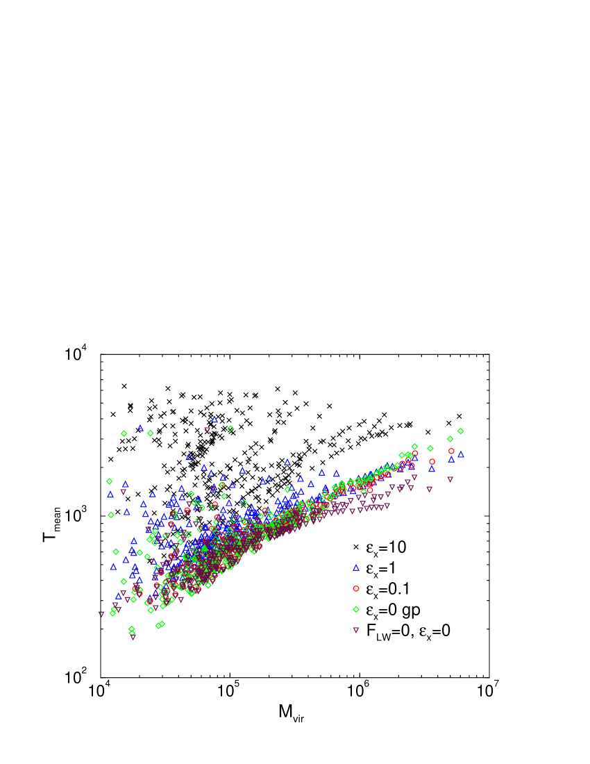
Figure 3: Mean gas-mass-weighted temperature as a function of virial mass for pregalactic clouds in the presence of a Lyman-Werner flux $F_{LW}=10^{-21}$  erg s^-1 cm^-2 Hz^-1 with no X-ray background ($\epsilon_{x}=0$ gp, green diamonds) and with a soft X-ray background whose relative normalizations are $\epsilon_{x}=0.1$ (red circles), 1 (blue triangles up) and 10 (black crosses). The case with no external radiation fields ($F_{LW}=0$, $\epsilon_{x}=0$) is represented by maroon down-pointing triangles. While most points fall along the virial relation, the $\epsilon_{x}=10$ case shows substantial heating from X-rays. In addition, cooling becomes important for the most massive objects.

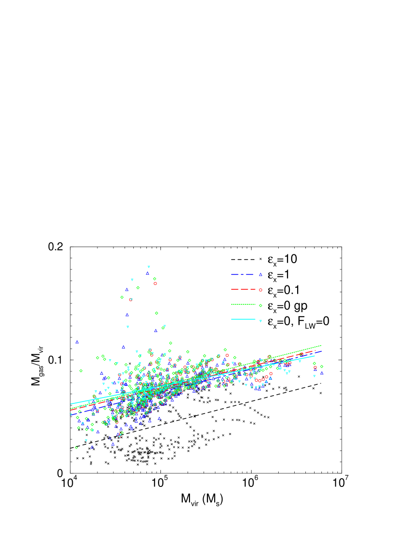
Figure 4: Gas fraction as a function of virial mass for clouds used in the analysis sample with Lyman-Werner flux $F_{LW}=10^{-21}$  erg s^-1 cm^-2 Hz^-1 and X-ray flux normalizations $\epsilon_{x}=0$ gp (green diamonds), $0.1$ (red circles), $1$ (blue triangles up), $10$ (black crosses). Maroon triangles down represent the $F_{LW}=0$, $\epsilon_{x}=0$ no radiation field case. Lines represent a mean regression analysis of the data set with respect to $\ln(M_{vir})$ for cases $\epsilon_{x}=0$ gp (green dotted), $0.1$(red long dashed), $1$(blue dot dashed), $10$(black dashed), and no radiation fields (maroon solid). While most objects fall near to the global ratio of 0.08, the $\epsilon_{x}=10$ case shows the effect of X-ray heating.

This X-ray heating of low mass clouds is more apparent in Figure 3 where we show the mean gas-mass-weighted temperature as a function of virial mass for pregalactic clouds exposed to a mean Lyman-Werner flux $F_{LW}=10^{-21}$  erg s^-1 cm^-2 Hz^-1 and X-ray flux varying over two orders of magnitude. We also show the $\epsilon_{x}=0$, $F_{LW}=0$ case (no background radiation fields) for comparison. For $\epsilon_{x}=1$ there is a modest increase in the mean temperature of the cloud for masses $M_{vir}\la 5\times 10^{5}M_{\odot}$; while for $\epsilon_{x}=10$ heating is dramatic with the mean gas temperature of the clouds raised well above their virial temperatures for $M_{vir}\la 10^{6}M_{\odot}$. In Figure 4 we investigate the consequences of this heating by plotting the cloud gas fraction $M_{gas}/M_{vir}$ as a function of $M_{vir}$ for halos in our data sample. The lines are from mean regression analyses of the data for each level of X-ray flux. Because there is large scatter in the data (correlation coefficients of only $\sim 0.5$ – $0.6$ ) the lines are only meant to guide the eye. However the decrease of gas fraction with increasing X-ray flux is clear with mean gas fractions given by $\sim 0.08$, $0.08$, $0.07$, and $0.04$ for X-ray flux normalizations $\epsilon_{x}=0$ gp, $0.1$, $1$, and $10$. The mean gas fractions for the low flux cases ($\epsilon_{x}\leq 1$) agree with the mean gas fraction ($0.08$) in the sample of halos not exposed to an external radiation field. This is consistent with most of the accreted gas being retained by the gravitational potential. However, heating in clouds experiencing the highest X-ray flux, such as those nearby to a newly formed miniquasar, causes a significant fraction of the gas to be evaporated into the surrounding intergalactic medium. Such effects have interesting consequences for re-ionization (Haiman, Abel & Madau 2001).

In Figure 3 we also see that X-ray enhanced cooling (positive feedback) occurs in the most massive peak in the simulation once its mass exceeds $2\times 10^{6}M_{\odot}$. Above this mass the mean temperature of the cloud exposed to both X-rays and the Lyman-Werner flux is noticeably lower than for the case with the Lyman-Werner flux alone and the mean temperature for a given mass decreases with increasing X-ray flux for $\epsilon_{x}\leq 1$. However, in all cases the mean temperature of the cloud lies above the limiting case with no radiation fields present. Furthermore the onset of cooling in the absence of background radiation fields occurs at $M_{vir}\sim 2-3\times 10^{5}M_{\odot}$, nearly an order of magnitude sooner. For the maximum X-ray flux level we consider, $\epsilon_{x}=10$, the situation is even worse. While cooling is apparent in the high mass objects ($M_{vir}\ga 10^{6}M_{\odot}$) it does not overcome the effects of X-ray heating and drop to its virial temperature until $M_{vir}>2\times 10^{6}M_{\odot}$. The mean temperature remains above that found for clouds exposed to the H₂ photodissociating flux alone ($\epsilon_{x}=0$ gp) up to the highest masses we find in our sample. Thus the presence of the X-ray background, even at these high levels, is insufficient to turn the negative feedback effect of the softer H₂ photodissociating UV background into a net positive one.

In Table 1 we present a quantitative example by comparing the mean masses, gas fractions, and temperatures found in our simulations for the most massive pregalactic cloud at redshift $z=20$ when it has grown through merging to a mass $M_{vir}\approx 5\times 10^{6}\,M_{\odot}$ ($T_{vir}\approx 5300$  K ) and radius $r_{vir}\approx 239$ pc. First in the absence of any X-ray flux we see that use of Galli & Palla (1998) cooling functions does increase cooling in this cloud producing about a $10\%$ reduction in its mean temperature over that obtained using cooling functions by Lepp & Shull (1983). Second, positive feedback does occur, but the effect is quite modest. Exposing the cloud to increasing levels of X-rays initially promotes cooling, as expected, causing the mean cloud temperature to decrease by $16\%$ for $\epsilon_{x}=0.1$ and $25\%$ for $\epsilon_{x}=1$ over the case with no X-rays and Galli & Palla cooling. However even in the maximal $\epsilon_{x}=1$ case, the mean temperature is $33\%$ higher in this cloud than in the cloud evolved from the same $z=30$ initial conditions but with no radiative feedback. Finally once the X-ray background becomes sufficiently strong, heating outside the core dominates. For $\epsilon_{x}=10$ the mean temperature of this cloud increased by $25\%$ over that of the cloud exposed to only the soft Lyman-Werner UV background and is more than a factor of $2$ above the mean temperature found for the cloud without radiative feedback. Furthermore, the fraction of gas retained by the gravitational potential decreased from $9-10\%$ of the cloud mass for $0\leq\epsilon_{x}\leq 1$ to $7\%$ for $\epsilon_{x}=10$, another reflection of the evaporation of X-ray heated gas from the outer radii in even this most massive cloud in our data set.

4 Cold Gas Fractions

A critical input parameter into semi-analytical structure formation and reionization models that include stellar feedback is the amount of gas in pregalactic objects that is available to form stars. In MBAI we used our data sample to determine both the fraction of gas in these low mass pregalactic objects that can cool $f_{c}$ and the fraction of gas $f_{cd}$ that can both cool and become dense in the presence of a mean Lyman-Werner H₂ photodissociating flux, thus quantifying the negative feedback effect of the soft UV radiation produced by the first stars on subsequent star formation. In this section we address how these gas fractions, $f_{c}$ and $f_{cd}$, change when an ionizing X-ray background is present and whether at some level they can reverse, as suggested by Haiman, Abel & Rees (2000), the negative feedback of the H₂ photodissociating flux.

As in MBAI we define $f_{c}$ and $f_{cd}$ in the following way:

$f_{c}$ is the fraction of total gas within the virial radius with temperature $T<0.5T_{vir}$ and gas density $\rho>1000\rho_{mean}$ where $\rho_{mean}$ is the mean gas density of the universe. This is the amount of gas within the cloud that has been able to cool due to molecular hydrogen cooling.

$f_{cd}$ is the fraction of total gas within the virial radius with temperature $T<0.5T_{vir}$ and gas density $\rho>10^{19}M_{\odot}\,\hbox{\rm Mpc${}^{-3}$}\sim 330$  cm^-3 . This is the fraction of gas within the cloud that is available for star formation.

The above criteria are applied on a cell by cell basis within the virial radius for each peak in the data sample described in §3. The temperature threshold has been chosen to ensure that the gas is substantially cooler than the virial temperature of the peak. The density threshold for cold, dense gas corresponds to the gas density at which the baryons become important to the gravitational potential and thus to the subsequent evolution of the core. The density threshold for the cooled gas is chosen to minimize the contribution of cold, infalling substructure and of cool gas within $r_{vir}$ but still outside the virial shock. (Please see MBAI Section 4 for more detail.)

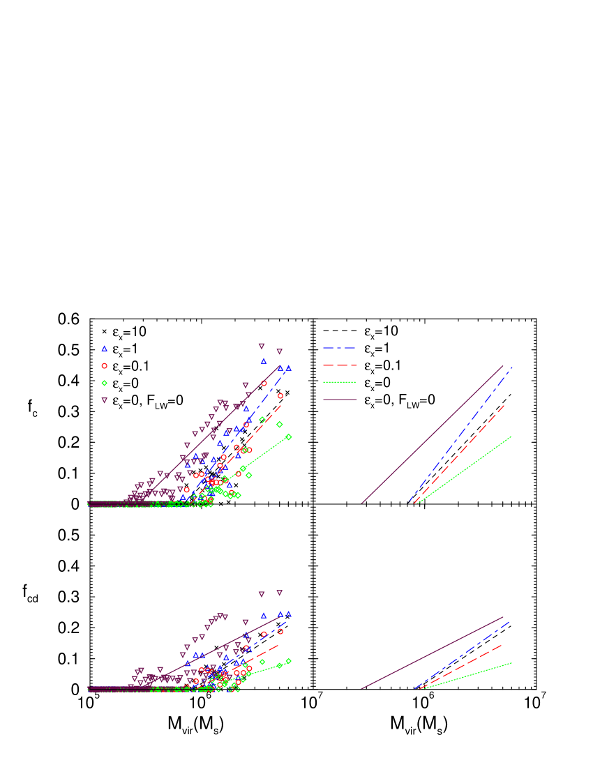
Figure 5: Fraction of cold gas within the virial radius as a function of cloud mass and X-ray flux for a soft Lyman-Werner UV background flux $F_{LW}=10^{-21}$  erg s^-1 cm^-2 Hz^-1 . In the top panels, we plot $f_{c}$, the fraction of gas that has cooled via H₂ cooling ($T<0.5T_{vir}$, $\rho>1000\rho_{mean}$) with $\rho_{mean}$ the mean baryonic density of the universe, while in the lower panels, we show $f_{cd}$, the fraction of cold, dense gas ($T<0.5T_{vir}$, $\rho>10^{19}$ $M_{\odot}$ Mpc^-3) available for star formation. Maroon triangles down show the limiting $F_{LW}=0$, $\epsilon=0$ case with no radiation fields present. Lines represent mean regression analyses of $f$ with the logarithm of the cloud mass for the cases $\epsilon_{x}=0$ gp (green dotted), $0.1$ (red long dashed), $1$ (blue dot dashed), $10$ (black dashed), and $F_{LW}=0$, $\epsilon_{x}=0$(maroon solid). The right-hand panels show the same fitted lines as in the left-hand panels, but plotted without data for clarity.

In Figure 5 we show the fraction of gas that can cool (top panel) and the fraction of gas that can both cool and become dense (bottom panel) and thus be available for star formation for each of our simulations ($\epsilon_{x}=0$ gp, $0$ ls, $0.1$, $1$, $10$ and $F_{LW}=0$ $\epsilon_{x}=0$). In Table 2 we show the results of a mean regression analysis of $f_{c}$ and $f_{cd}$ with the logarithm of the cloud mass,

$$f_{i}=B_{i}\ln(M/M_{i})$$ (11)

for $i=c$ (cooled gas), $i=cd$ (cold, dense gas) and $M>M_{i}$. $M_{i}$ and $K_{i}$ ($i=c,cd$) are the mass thresholds and correlation coefficients for each process derived from the regression analyses. We again see that the fractions of gas that can cool ($K_{c}\sim 0.8$) or cool and become dense ($K_{cd}\sim 0.9$) are highly correlated with the mass of the pregalactic cloud, although as discussed in §3 the reduced scatter in the high mass end is partially due to the small number of independent high mass peaks in our simulation volume.

The most striking aspect of Figure 5 is that the positive feedback of an X-ray background on structure formation is remarkably weak, even though we vary the X-ray intensity by two orders of magnitude. As the relative normalization of the X-ray flux is increased to $\epsilon_{x}=1$, the mass threshold at which gas can cool or cool and become dense (and thus available for star formation) does decrease as expected if the positive effect of X-rays on H₂ formation partially compensates for the H₂ destruction by the soft UV Lyman-Werner photons, but only modestly. This decrease in the mass threshold for gas to cool, from $\sim 8.5\times 10^{5}\,M_{\odot}$ for $\epsilon_{x}=0$ to $\sim 7\times 10^{5}\,M_{\odot}$ for $\epsilon_{x}=1$, and for gas to both cool and become dense, from $10^{6}M_{\odot}$ for $\epsilon_{x}=0$ to $8\times 10^{5}M_{\odot}$ for $\epsilon_{x}=1$, caused by the presence of the X-ray background is much less than the decrease from $10^{6}\,M_{\odot}$ to $4.2\times 10^{5}\,M_{\odot}$ in these thresholds found in MBAI caused by an order of magnitude reduction in the H₂ photodissociating flux (from $10^{-21}$ to $10^{-22}$  erg s^-1 cm^-2 Hz^-1 ) and the mass thresholds for the case with $\epsilon_{x}=1$ are still a factor $\ga 3$ higher than for the case when no Lyman-Werner UV background is present. Thus, in contrast to Haiman, Abel & Rees (2001), we find that the positive effect of the X-rays is too weak to overcome the delay in cooling caused by the H₂ photodissociating flux. As the X-ray flux is increased further to $\epsilon_{x}=10$, the mass threshold for cooling increases again, because at these X-ray flux levels the weakly enhanced cooling must compete with significant X-ray heating of the gas within the cloud. This is consistent with the fact that the redshift when maximal refinement first occurs, i.e. when the first peak “collapses” in the simulation volume, increases with increasing X-ray flux for $0\leq\epsilon\leq 1$ ($z=21.5$, $22.6$, $23.2$ for $\epsilon=0$ gp and ls, $0.1$, $1$ respectively) , decreases slightly ($z=23$) for $\epsilon=10$, but in all cases occurs significantly later than $z=26.5$, the redshift of maximal refinement in our no radiation field control simulation.

The effect of the X-ray background on the amount of gas that can cool and become dense once cooling commences is more significant, but still small. In Figure 5 and Table 2 we see that the regression coefficients $B_{i}$, $i=c,cd$ increase by as much as a factor $\sim 2$ with increasing X-ray flux for $\epsilon_{x}\leq 1$. This trend reverses for the highest flux level we consider ($\epsilon_{x}=10$) because then X-ray heating of the gas within the cloud is important, reducing the fraction of gas that has been able to cool to temperatures significantly below the cloud’s virial temperature to values similar to that obtained with $\epsilon_{x}=0.1$, an X-ray flux two orders of magnitude smaller. The slopes for the two most intense X-ray flux levels ($B_{c}=0.17-0.20$ and $B_{cd}\sim 0.1$) are also somewhat steeper than those ($B_{c}=0.15$ and $B_{cd}\sim 0.08$) found in our $F_{LW}=0$, $\epsilon_{x}=0$ control simulation. Better statistics are needed for high mass clouds to determine whether this steepening is significant. Note, however, that in the most massive peak at $z=20$ the fraction of gas available for star formation in the $F_{LW}=0$ control simulation ($0.31$) is still significantly higher than the maximum found ($0.24$) for that cloud when both X-rays and the soft Lyman-Werner background are present. We also find that use of the Galli & Palla (1998) rather than Lepp & Shull (1984) fit for the H₂ cooling function increases the slope of the fitting function for the cold and dense gas available for star formation by $\sim 30\%$. As in MBAI we attribute the softer slope for the $\epsilon_{x}=0$ gp(ls) cases to poor statistics and increased scatter near the cooling threshold.

5 Internal Cloud Properties

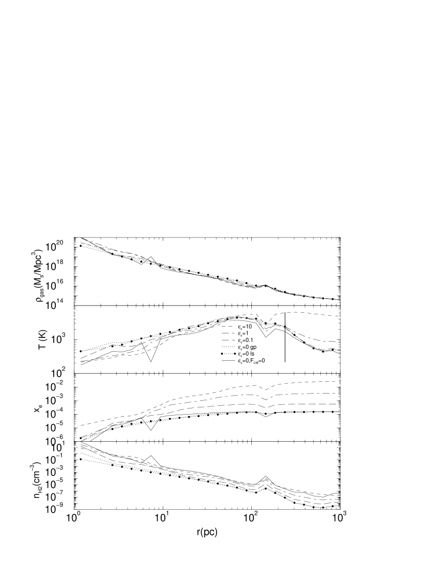
Figure 6: Radial profiles of (from top to bottom) the gas density $\rho_{gas}$, temperature $T$, electron abundance $x_{e}$ and H₂ number density $n_{H2}$ for a pregalactic cloud of mass $5\times 10^{6}M_{\odot}$ at $z=20$ with $F_{LW}=10^{-21}$  erg s^-1 cm^-2 Hz^-1 and relative X-ray flux normalizations $\epsilon_{x}=0$ gp (dotted), $0$ ls (dotted with filled circles), $0.1$ (long dashed), $1$ (dot-dashed), and $10$ (dashed) and with no background radiation fields (solid). The vertical line denotes the virial radius $r_{vir}=239$ pc.

We can gain a better understanding of the physical processes at work when pregalactic structure is exposed to both X-ray and Lyman-Werner UV backgrounds (and hope to explain why the effect is so mild) by studying the internal structure of a collapsing cloud. In this section we compare radial profiles of physical properties for a single cloud for the various levels of X-ray and soft UV flux used in our simulations. Guided by Figure 3 and Table 1, we choose the most massive peak in our simulations ($M_{vir}\sim 5\times 10^{6}M_{\odot}$) at $z=20$ for these comparison studies. In Figure 6 we present the spherically averaged radial profiles of the gas density $\rho_{gas}$, temperature $T$, electron abundance $x_{e}=n_{e}/(n_{HI}+n_{HII})$ and H₂ number density $n_{H2}$ for this cloud. The virial radius $r_{vir}=239$ pc is denoted by a vertical line in the gas temperature panel. The enhancement seen in the gas density and H₂ number density (corresponding to the dip in temperature and electron abundance) for radii $100<r<200$ pc is the characteristic signature of infalling substructure. As is often the case in hierarchical models, the most massive peak lies within a dynamically active filament in the simulation volume where mergers are common and, in fact, has only recently formed ($z=20.5$) through the completion of the merger of two nearly equal mass subcomponents (see the massive peaks in MBAI, Figure 5).

The most remarkable feature of the profiles in Figure 6 (and one of the main results of this paper) is how weakly the X-rays affect the cloud properties, particularly the gas density and temperature, even though we vary the X-ray flux by two orders of magnitude. The gas density profiles at radii $r>10$ pc for the various X-ray fluxes are nearly indistinguishable, although they do steepen somewhat for $\epsilon_{x}=1$ and $10$ and approach more closely the density profile for the no radiation field case ($F_{LW}=0$, $\epsilon_{x}=0$). The gas density profiles differ most in the inner $10$ pc of the structure. The density tends to increase with increasing X-ray flux for fixed soft UV flux $F_{LW}=10^{-21}$  erg s^-1 cm^-2 Hz^-1 . However, it appears to saturate for $\epsilon_{x}=1$ with the profile flattening significantly for $\epsilon_{x}=10$, the highest X-ray flux case. While the maximum density shown for the $\epsilon_{x}=1$ simulation is similar to that for the case with no radiation field, substructure is much more obvious in the latter. This is a consequence of the lower mass threshold (See §4) for a cloud to become dense and collapse. Thus infalling substructure is more highly evolved (colder and denser) when no background fields are present.

The temperature panel of Figure 6 is particularly interesting. We find that the dominant effect of the higher two X-ray flux levels is to heat and (from the third panel) partially ionize the lower density gas near the virial radius. This serves to weaken the accretion shock as the X-ray flux is increased until for our extreme case ($\epsilon_{x}=10$), the temperature of the lower density IGM exceeds the virial temperature of the cloud. Interior to the accretion shock and over most of the object’s extent ($10\la r\la 200$ pc), the temperature profiles are remarkably similar. The onset of cooling within the cloud occurs near $r\sim 60$ pc for all the simulations where the density has reached $\rho\sim 3\times 10^{16}$ Mpc^-3 ($n\sim 1$  cm^-3 ), in agreement with Haiman, Abel & Rees (2000). The temperature does decrease modestly with increasing X-ray flux demonstrating positive feedback. As the X-ray flux is increased, thereby increasing the electron fraction through secondary ionizations, there is more H₂ coolant produced so that the cloud cools more efficiently (See the lower two panels of Figure 6). Within $10$ pc sufficient H₂ has formed by $z=20$ to drive the temperature to its minimum for molecular hydrogen alone, $\sim 200\,{\rm K\ }$, in the high X-ray flux cases ($\epsilon_{x}=1$, $10$) and the no radiation field case ($F_{LW}=0$,$\epsilon_{x}=0$). The temperature is close to its minimum for the other cases ($\epsilon_{x}=0.1$,$0$ ls, $0$ gp). Again, the major difference between the profiles is that in the $F_{LW}=0$, $\epsilon_{x}=0$ case infalling substructure at $r\sim 7.4$ pc is clearly seen; while it is not seen in any of the profiles that include Lyman-Werner and X-ray backgrounds, even those with the highest X-ray fluxes (see MBAI for more discussion of substructure in halos, in particular Figure 5 of that paper). For the no radiation field case this substructure has formed sufficient molecular hydrogen ($n_{H2}\sim 0.5$) to cool to $\sim 200$  K (the minimum temperature for H₂ cooling) and reach high density; while in all other cases the cooling has been delayed within the substructure by the H₂ photodissociating soft UV component of the background radiation field.

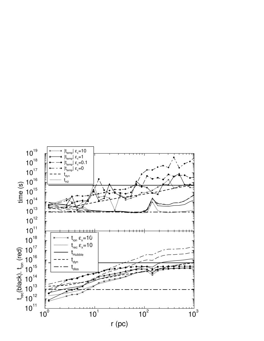
Figure 7: Radial profiles of timescales relevant to cooling and collapse at z=20 for the same cloud as in Figure 6. In the top panel we plot $t_{temp}$ as lines with points for the four values of $\epsilon_{x}$. These times are generally longer or equal to the dynamical time (shown as a dashed line for just one model because all four cases are quite similar). On the other hand, the H₂ formation times for the four cases (same line styles as for $t_{temp}$ but without the points are very close to the H₂ photodissociation time which is ploted as a dot-dashed line. In the bottom panel, we compare the ionization and recombination times for the four values of $\epsilon_{x}$ using the same line convention as in the top panel ($t_{ion}$ is plotted with symbols, while $t_{rec}$ is not). Note that one cannot define $t_{ion}$ for the $\epsilon_{x}=0$ case so we do not plot it. The two time-scales are comparable either for high densities (i.e. small radii) or large values of the X-ray flux, $\epsilon_{x}$.

In Figure 7 we plot timescales important to cloud cooling and collapse for the same pregalactic cloud, redshift, and X-ray background levels used in Figure 6. In the top panel we show the H₂ formation time $t_{H2}$, H₂ photodissociation time $t_{diss}$, and the magnitude of the timescale for temperature change (loosely, the “cooling” time) $|t_{temp}|$ compared to the dynamical time $t_{dyn}$ and Hubble time $t_{Hubble}$. In the lower panel we compare the recombination time $t_{rec}$ and ionization time $t_{ion}$ to $t_{Hubble}$ and $t_{diss}$. All of the timescales except $t_{temp}$ and $t_{ion}$ are given by the equations in MBAI. We repeat them here for completeness:

$$t_{dyn}=\biggl{(}\frac{3\pi}{16G\rho}\biggr{)}^{1/2},$$

$$t_{Hubble}=\frac{2}{3H_{0}}(\Omega_{0}(1+z)^{3})^{-1/2},$$

$$t_{H2}=\frac{n_{H2}}{k_{7}n_{HI}n_{e}},$$ (12)

$$t_{diss}=k_{diss}^{-1}=9\times 10^{-9}/F_{LW},$$

$$t_{rec}=7.7\times 10^{9}T^{0.64}/n_{e},$$

where $G$ is the gravitational constant, $\rho$ is the total density, $H_{0}$ is the Hubble constant today, $\Omega_{0}$ is the fraction of the critical density carried in matter today, $z$ is the redshift, $n_{H2}$, $n_{HI}$, and $n_{e}$ are the molecular hydrogen, neutral hydrogen, and electron number densities, $F_{LW}$ is the mean Lyman-Werner UV flux, $T$ is the temperature and $k_{7}\approx 1.8\times 10^{-18}T^{0.88}$ cm³ s^-1 over this temperature range.

We have defined a timescale for temperature change due to radiative processes (very loosely, a generalization of the “cooling” time) that includes both radiative cooling and the effects of heating by X-ray photo-electrons

$$t_{temp}=\frac{e}{de/dt|_{r}}$$ (13)

where $e$ is the thermal energy of the gas and $de/dt|_{r}$ is its rate of change due to radiative processes, such that $t_{temp}>0$ indicates net cooling, while $t_{temp}<0$ indicates net heating. The sharp fluctuations in $|t_{temp}|$ seen in Figure 7 when ionizing X-rays are present result from the competition between regions where heating versus cooling dominates within the radial shells. Most often the net effect of the X-ray flux on the outer parts of the cloud is to heat the gas; while net cooling is more likely in the interior regions.

The ionization time is given by

$$t_{ion}=\frac{n_{e}}{\epsilon_{x}n_{HI}R}$$ (14)

where $n_{e}$, $n_{HI}$ and $n_{HeI}$ are the electron, neutral hydrogen and neutral helium number densities, and $R=k_{24}+(n_{HeI}/n_{H})k_{26}$ is the ionization rate in the gas (See Equations 8 and 9). The ionization rate is dominated by the production of secondary electrons from H $\rm\scriptstyle I\$produced by primaries from the X-ray photoionization of He $\rm\scriptstyle I\$. Although we evolve the true ionization fraction $x=n_{HII}/(n_{HI}+n_{HII})$ at each timestep in our calculation, $n_{HII}\approx n_{e}$ in our simulations so that the ionization fraction $x$ is well approximated by the electron abundance $x_{e}$ shown in the third panel of Figure 6. From that figure we see that the ionization fraction remains small, $x\la 0.02$, within the cloud, even for the highest X-ray flux level. Thus $R$ in Equation 14 is nearly constant, $R\sim 2.6\times 10^{-18}$ s^-1.

Figure 7 shows that for all the cases with a soft UV Lyman-Werner background, i.e. with or without an extra ionizing X-ray component, the pregalactic cloud is in photodissociation equilibrium over much of its interior ($10\la r\la 100$ pc). Thus the H₂ number density is well approximated by its photodissociation equilibrium value

$$n_{H2}^{equil}\approx\frac{k_{7}n_{HI}n_{e}}{k_{diss}}.$$ (15)

The photodissociation timescale is much shorter than either the recombination or ionization times in this region. In addition, for the cases with the most X-ray flux, the cloud is also close to ionization equilibrium. However, the recombination rate is still slightly faster than the ionization rate. We can use the fact that the cloud is both in photodissociation equilibrium and in approximate ionization equilibrium over these radii ($10\la r\la 100$ pc) to understand the scaling properties of $n_{H2}$ seen in the bottom panel of Figure 6. Since $n_{HII}\approx n_{e}$ ionization equilibrium implies that the electron number density $n_{e}^{equil}$ scales as

$$n_{e}^{equil}\propto(\epsilon_{x}F_{LW}n_{HI})^{1/2}T^{0.32}$$ (16)

Thus for interior regions where both ionization and photodissociation equilibrium hold we may substitute Equations 2 and 16 and into Equation 15 (for fixed $F_{LW}$) to obtain

$$n_{H2}^{equil}\propto\epsilon_{x}^{1/2}n_{HI}^{3/2}T^{1.2}$$ (17)

Since at these radii Figure 6 shows that the density and temperature profiles are similar, we expect the amount of H₂ coolant to scale roughly as $n_{H2}\sim\epsilon_{x}^{1/2}$. Thus changing the X-ray flux by a factor $100$ only changes the amount of H₂ coolant by about a factor of $10$ (as seen in the bottom panel of Figure 6). Only in the core region do we see ionization dominate for the high X-ray flux cases; however by this redshift (see Figure 6) the core has already maximally cooled. X-ray enhanced production of molecular hydrogen in this region will not promote additional cooling. Thus the positive feedback effect of X-rays, while present, is too slow to dramatically reverse the delay in cooling and collapse caused by the rapid photodissociation of H₂ in these systems. Note also that the dynamical collapse time is faster than recombination or ionization times over most of cooling region for $\epsilon_{x}=0.1$ and comparable to $t_{rec}$ and $t_{dyn}$ for $\epsilon_{x}=1$, so density evolution can not be ignored.

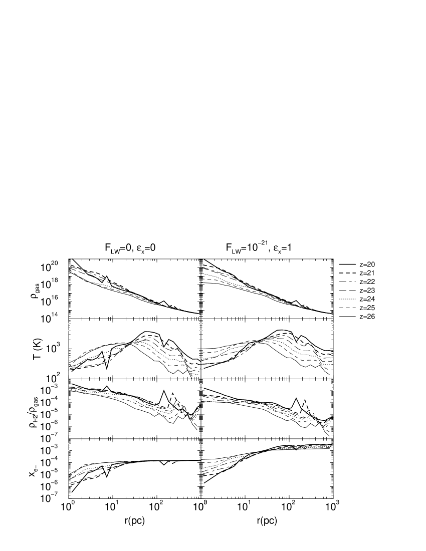
Figure 8: Evolution of radial profiles of (from top to bottom) the gas density $\rho_{gas}$, temperature $T$, H₂ mass fraction $\rho_{H2}/\rho_{gas}$ and electron abundance $x_{e}$ from $z=26$ to $z=20$ for the pregalactic cloud of Figure 6. Left panels show the case with no background radiation fields present ($F_{LW}=0$, $\epsilon_{x}=0$); while right panels show the case with maximal positive feedback ($F_{LW}=10^{-21}$  erg s^-1 cm^-2 Hz^-1 , $\epsilon_{x}=1$). Lines denote redshifts $z=26$(thin solid), $25$(thin dashed), $24$(dotted), $23$(long dashed), $22$(dot dashed), $21$(thick dashed), and $20$(thick solid).

We can check that this is actually the case for our collapsing cloud by tracking the evolution of its internal properties. In Figure 8 we show the evolution of the density $\rho_{gas}$, temperature $T$, H₂ mass fraction $\rho_{H2}/\rho_{gas}$, and electron abundance $x_{e}$ from redshifts $26\geq z\geq 20$ for the case with maximal positive feedback $\epsilon_{x}=1$ (right panels) and the case with no background radiation fields $F_{LW}=0$,$\epsilon_{x}=0$ (left panels). For the $\epsilon_{x}=1$ case at high redshift $z\sim 26$, the electron fraction is not significantly enhanced in the core region. The photodissociation timescale is much shorter than all other timescales in the problem so that the level of H₂ coolant is controlled by its photodissociation equilbrium value. At this redshift the cloud temperature is still high ($\sim 1000$  K ), the H₂ mass fraction is near its critical value (see MBAI) and the cloud has just begun to cool. The density profile in the core is still roughly constant, as expected for a cloud before collapse, and gradually steepens into a characteristic $r^{-2}$ form by $z\sim 23$. In contrast, the control case with no radiative feedback evolves much more quickly. By $z=26$ the fraction of molecular hydrogen, whose build up in this case is not regulated by photodissociation, is $\ga 10^{-3}$, more than an order of magnitude greater than for the $\epsilon_{x}=1$ case at the same redshift. The temperature in the core is $\sim 450$  K at $z=26.5$ and has cooled to its minimum value by $z=26$. The cloud has collapsed as indicated by the steep core density profile. Densities in the core are more than an order of magnitude greater than those for the case with radiative feedback. We also see from Figure 8 that the electron abundance near the virial radius is an order of magnitude greater for the case with X-rays than without. Thus the dominant effect of the X-rays is to partially ionize the lower density regions. We also see in both cases evidence for and the importance of growth through merging of smaller substructures in the formation of the cloud.

In the outer low density region $r\ga r_{vir}$, we see enhanced H₂ formation caused by the increased electron fraction; however, the levels of H₂ remain below the critical threshold (see MBAI) for cooling to be important. We also caution the reader that the H₂ fractions for the low density regions shown in Figure 6 and the right panel of Figure 8 should be considered conservative upper limits on the amount of coolant present because H^- photodetachment, which we ignore, is no longer negligible once $n_{HI}\la 0.045$ ($\rho_{gas}\la 6\times 10^{15}\,M_{\odot}\,\hbox{\rm Mpc${}^{-3}$}$). We find that the dominant effect of the X-rays at these large radii is to heat and partially ionize the intergalactic medium, in qualitative agreement with recent work on the IGM by Venkatesan et al. (2001).

6 Summary

In this paper we used high resolution numerical simulations to investigate the effect of radiative feedback on the formation of $10^{5}$ –$10^{7}M_{\odot}$ pregalactic clouds when the radiation spectrum extends to energies above the Lyman limit ($\ga 1$ keV). Such an ionizing X-ray component is expected if the initial mass function of the first luminous sources contains an early generation of miniquasars or very massive stars. The range of pregalactic objects we consider is important because they are large enough to form molecular hydrogen, but too small to cool by hydrogen line cooling. Thus any process that affects the amount of H₂ coolant within the cloud affects its ability to cool, lose pressure support and collapse to high density. The soft, UV flux in the $11$–$13$ eV Lyman-Werner band produced by the first stars can destroy the fragile H₂ in these objects delaying subsequent collapse and star formation until later redshifts when the objects have evolved to larger masses. We test whether the presence of ionizing X-rays can mitigate or even reverse this effect by increasing the electron fraction in the gas and thus enhancing the formation of molecular hydrogen coolant. Since the relative amplitude of the X-ray to soft UV components in the background spectrum of the first luminous sources is unknown, we study four cases with relative X-ray normalizations ranging from zero to ten for mean soft UV flux at $12.86$ eV of $10^{-21}$  erg s^-1 cm^-2 Hz^-1 . We compare these results to the case with no background radiation fields. We draw our initial conditions from a $\Lambda$CDM cosmological model. The simulations evolve the nonequilibrium rate equations for $9$ species of hydrogen and helium including the effects of secondary electrons. A summary of our main findings are as follows:

• Ionizing X-rays do have a positive effect on subsequent structure formation, but the effect is very mild. Even in the presence of X-rays photodissociation is rapid delaying the collapse of the cloud until later redshifts when larger objects have collapsed.

• The mass thresholds for gas to cool and for gas to cool and become dense decrease only weakly with increasing X-ray flux up to relative X-ray normalization $\epsilon=1$ when compared to the case with only a soft UV radiation field, but remain $\ga$ a factor three more massive than the mass collapse threshold found when no radiation fields were present. Equivalently, the redshift for collapse decreases weakly with increasing X-ray flux up to $\epsilon_{x}=1$ from that for the case with only a soft UV radiation field, but collapse occurs significantly later than in the case with no background radiation field.

• The fraction of gas that can cool or cool and become dense (and thus become available for star formation) within a cloud increases with increasing X-ray flux. We fit these fractions with a simple fitting formula (Equation 11) that increases logarithmically with cloud mass and find that the slope of this fitting formula increases by as much as a factor $\sim 2$ with increasing X-ray flux for X-ray normalizations $\epsilon_{x}\leq 1$.

• The weak positive effect of the ionizing X-rays appears maximal for relative normalization $\epsilon_{x}=1$. For significantly higher X-ray fluxes the positive trends described in the previous two items is reversed. Heating becomes important both within the cloud and in the surrounding intergalactic medium thus weakening the characteristic accretion shock near the virial radius. The mean temperature of the cloud is raised well above its virial temperature causing a significant fraction of the gas to be evaporated into the surrounding intergalactic medium.

We conclude that although an early X-ray background from quasars or mini-quasars does enhance cooling in pregalactic objects, the effect is weaker than found in previous studies that did not follow the evolution of the collapsing cloud. The net impact on subsequent structure formation is still negative due to photodissociation of the H₂ coolant by the soft UV radiation spectrum of the first stellar sources, and the pattern of subsequent structure formation is only weakly changed by including an ionizing X-ray component. We should point out that that we have not included star formation and its subsequent effect on the forming halos in these simulations (except insofar as we have modelled the radiative background), so obviously more work on this subject is required. In this context, it is interesting to note that Ricotti et al. (2002a, 2002b) have simulated star formation and radiative transfer in somewhat more massive halos (albeit with a mass resolution 100 times lower than used here) and find a self-regulated feedback loop that includes positive feedback.

Together with the findings of MBAI our results suggest that radiative feedback from cosmological radiation backrounds have subtle effects on the formation of luminous objects within the micro–galaxies. The negative feedback of a soft UV background may change the minimum mass of a dark halo within which gas may cool by a factor of a few. However, even in the most extreme cases considered the first objects to form rely on molecular hydrogen as coolant. Hence, our results do not justify the neglect of halos cooling by molecular hydrogen in all current studies of galaxy formation.

We found that heating from an early X-ray background only slightly modifies the temperature and density profiles of halos at the time when a cool core is first formed in their centers. One may speculate that such temperature variations may lead to varying accretion rates onto the proto–star which will form within them (Abel, Bryan & Norman 2002). If so early radiation backgrounds may influence the spectrum of initial masses of Population III stars. To answer such detailed questions will rely on carrying out yet higher resolution simulations than the ones presented here.

This work is supported in part by National Science Foundation grant ACI-9619019. The computations used the SGI Origin2000 at the National Center for Supercomputing Applications. M.E.M. gratefully acknowledges the hospitality and support of the MIT Center for Space Research where most of this work was done.

Figure 1: (upper) Mean temperature as a function of virial mass for pregalactic clouds in the presence of a Lyman-Werner flux $F_{LW}=10^{-21}$  erg s^-1 cm^-2 Hz^-1 . (lower) Virial mass as a function of redshift $z$ for pregalactic clouds in the presence of a Lyman-Werner flux $F_{LW}=10^{-21}$  erg s^-1 cm^-2 Hz^-1 . Diamonds (pluses) represent halos simulated using Galli & Palla (Lepp & Shull) cooling functions.

Figure 2: Virial mass as a function of redshift for peaks used in the analysis sample with Lyman-Werner flux $F_{LW}=10^{-21}$  erg s^-1 cm^-2 Hz^-1 and X-ray flux normalizations of $\epsilon_{x}=0$ gp (diamonds), $0.1$ (circles), $1$ (triangles) and $10$ (squares).

$\epsilon_{x}$ $M_{vir}$ $M_{gas}$ $M_{gas}/M_{vir}$ $T_{mean}$ $T_{vir}$ $10^{6}\,M_{\odot}$ $10^{6}\,M_{\odot}$ K K $0$ ls $5.0$ $0.50$ $0.10$ $3200$ $5300$ $0$ gp $5.0$ $0.49$ $0.10$ $3000$ $5300$ $0.1$ $5.1$ $0.48$ $0.09$ $2500$ $5400$ $1$ $5.1$ $0.47$ $0.09$ $2200$ $5400$ $10$ $4.9$ $0.37$ $0.07$ $3800$ $5200$ none $5.0$ $0.43$ $0.09$ $1700$ $5300$

Table 1: Mean properties of the most massive peak at redshift $z=20$ exposed to a mean Lyman-Werner flux $F_{LW}=10^{-21}$  erg s^-1 cm^-2 Hz^-1 and ionizing X-ray background whose spectrum is given by Equation 3 where $\epsilon_{x}$ denotes the relative X-ray flux normalization. The row labeled “none” denotes the $F_{LW}=0$, $\epsilon_{x}=0$ case.

$\epsilon_{x}$ $B_{c}$ $M_{c}$ $K_{c}$ $B_{cd}$ $M_{cd}$ $K_{cd}$ $10^{5}M_{\odot}$ $10^{5}M_{\odot}$ $0$ ls $0.077$ $8.5$ $0.87$ $0.033$ $10$ $0.83$ $0$ gp $0.113$ $8.6$ $0.86$ $0.047$ $9.5$ $0.84$ $0.1$ $0.171$ $7.9$ $0.87$ $0.084$ $8.8$ $0.79$ $1$ $0.205$ $7.0$ $0.90$ $0.111$ $8.0$ $0.79$ $10$ $0.166$ $6.9$ $0.85$ $0.105$ $8.3$ $0.80$ none $0.153$ $2.7$ $0.94$ $0.080$ $2.7$ $0.82$

Table 2: Coefficients determined by a mean regression analysis assuming the functional form $f_{i}=B_{i}\ln(M/M_{i})$ ($M>M_{i}$) where $f_{i}$ are the fractions of cold gas ($i=c$) and cold, dense gas ($i=cd$) formed in pregalactic clouds when both soft UV Lyman-Werner and ionizing X-ray backgrounds are present. The mean Lyman-Werner flux is fixed at $F_{LW}=10^{-21}$  erg s^-1 cm^-2 Hz^-1 . Relative X-ray normalizations are given by $\epsilon_{x}$, $K_{i}$ are the respective correlation coefficients for the fits, ls (gp) denotes the use of Lepp & Shull (Galli & Palla) cooling functions, and “none” labels the $F_{LW}=0$, $\epsilon_{x}=0$ case.

References

- [Abel et al. (1997)] Abel, T., Anninos, P., Zhang, Y., & Norman, M. L. 1997, New Astronomy, 2, 181
- [Abel et al. (1998)] Abel, T., Anninos, P., Zhang, Y., & Norman, M. L. 1998, ApJ, 508, 518
- [Abel, Bryan & Norman (2000)] Abel, T. , Bryan, G.L., & Norman, M.L. 2000, ApJ, 540, 39
- [Abel, Bryan & Norman (2002)] Abel, T., Bryan, G.L., & Norman, M.L. 2002, Science, 295, 93
- [Bromm, Coppi & Larson (2001)] Bromm, V., Coppi, P.S. & Larson, R.B. 2001, ApJ, 563, ? (in press) preprint astro-ph/0102503
- [Barkana & Loeb (2001)] Barkana, R. & Loeb, A. 2001, Physics Reports, 349, 125
- [Ciardi, Ferrara & Abel (2000)] Ciardi, B., Ferrara, A. & Abel, T. 2000, ApJ, 533, 594
- [Ciardi et al. (2000)] Ciardi, G., Ferrara, A., Governato, f. & Jenkins, A. 2000, MNRAS, 314, 611
- [Dekel & Rees (1987)] Dekel, A. & Rees, M.J. 1987, Nature, 326, 455
- [Eisenstein & Hu (1998)] Eisenstein, D.J. & Hu, W. 1998, ApJ, 496, 605
- [Eisenstein & Hut (1998)] Eisenstein, D.J. & Hut, P. 1998, ApJ, 498,137
- [Ellison et al. (1999)] Ellison, S.L, Lewis, G.F., Pettini, M., Chaffee, F.H., Irwin, M.J. 1999, ApJ, 520, 456
- [Ellison et al. (2000)] Ellison, S. L., Songaila, A., Schaye, J. & Pettini, M. 2000, AJ, 120, 1175
- [Fan et al. (2001)] Fan, X., Narayanan, V.K., Strauss, M.A., White, R.L., Becker, R.H., Pentericci, L., & Rix, H.-W. 2001, AJ submitted, astro-ph/0111184
- [Fuller & Couchman (2000)] Fuller, T.M. & Couchman, H.M.P. 2000, ApJ, 544, 6
- [Fryer, Woosley & Heger (2001)] Fryer, C. L., Woosley, S.E. & Heger, A. 2001, ApJ, 550, 372
- [Galli & Palla (1998)] Galli, D. & Palla, F. 1998, A &A, 335, 403
- [Glover & Brand (2001)] Glover, S.C.O. & Brand, P.W.J.L. 2001, MNRAS, 321, 385
- [Haiman, Abel & Madau (2001)] Haiman, Z., Abel, T. & Madau, P. 2001, ApJ, 551, 599
- [Haiman, Abel & Rees (2000)] Haiman, Z., Abel, T. & Rees, M.J. 2000, ApJ, 534, 11
- [Haiman, Rees & Loeb (1996)] Haiman, Z., Rees, M.J. & Loeb, A. 1996, ApJ, 467, 522
- [Haiman, Rees & Loeb (1997)] Haiman, Z., Rees, M.J. & Loeb, A. 1997, ApJ, 476, 458
- [Haiman, Thoul & Loeb (1996)] Hiaman, Z., Thoul, A.A., & Loeb, A. 1996, ApJ, 464, 523
- [Hu et al. (2002)] Hu, E.M, Cowie, L.L., McMahon, R.J., Capak, P., Iwamuro, F., Kneib, J.-P., Maihara, T., Motohara, K. 2002, ApJl, submitted, preprint astro-ph/0203091
- [Lepp & Shull (1983)] Lepp, S. & Shull, J.M. 1983, ApJ, 270, 578
- [Machacek, Bryan & Abel (2001)] Machacek, M.E., Bryan, G.L. & Abel, T. 2001, ApJ, 548, 509
- [Madau, Ferrara & Rees (2001)] Madau, P., Ferrara, A. & Rees, M.J. 2001, ApJ, 555, 92
- [Nakamura & Umemura (2001)] Nakamura, F & Umemura, M. 2001, ApJ, 548, 19
- [Oh (2001)] Oh, S.P. 2001, ApJ, 553, 499
- [Oh & Haiman (2001)] Oh, S.P. & Haiman, Z. 2001, preprint astro-ph/0007351
- [Oh et al. (2001)] Oh, S.P., Nollett, K.M., Madau, P. & Wasserburg, G.J. 2001, ApJ, submitted preprint astro-ph/0109400
- [Omukai & Nishi (1998)] Omukai, K. & Nishi, R. 1998, ApJ, 508, 141
- [Reimers et al. (1997)] Reimers, D., Kohler, S., Wisotzki, L., Groote, D., Rodriquez-Pascal, P., & Wamsteker, W. 1997, A & A, 327, 890
- [Ricotti, Gnedin & Shull (2001)] Ricotti, M., Gnedin, N. & Shull, J.M. 2001, ApJ, 560, 580
- [Ricotti et al. (2002a)] Ricotti, M., Gnedin, N. & Shull, J.M. 2002a, ApJ, in press preprint astro-ph/0110431v2
- [Ricotti et al. (2002b)] Ricotti, M., Gnedin, N. & Shull, J. M. 2002b, ApJ, in press preprint astro-ph/0110432v2
- [Schaye et al. (2000)] Schaye, J., Rauch, M., Sargent, W.L.W., Kim, T.-S. 2000, ApJ, 541, L1
- [Schneider et al. (2001)] Schneider, R., Ferrara, A., Natarajan, P., & Omukai, K. 2001, preprint astro-ph/0111341
- [Tegmark et al. (1997)] Tegmark, M., Silk, J., Rees, M.J., Blanchard, A., Abel, T., & Palla, F. 1997, ApJ, 474, 1
- [Tozzi et al. (2000)] Tozzi, P., Madau,P., Meiksin, A. & Rees, M.J 2000, ApJ, 528, 597
- [Shull & Van Steenberg (1985)] Shull, J.M. & Van Steenberg, M.E. 1985, ApJ, 298, 268
- [Venkatesan, Giroux & Shull (2001)] Venkatesan, A., Giroux, M.L., & Shull, J.M. 2001, ApJ, in press, preprint astro-ph/0108168
- [Vernier et al. 1996] Vernier, D.A., Ferland, G. J., Korista, K.T., & Yakovlev, D.G. 1996, ApJ, 465, 487