Detection of Solar-like Oscillations in the G7 Giant Star $\xi$ Hya

We report the firm discovery of solar-like oscillations in a giant star. We monitored the star $\xi$ Hya (G7III) continuously during one month with the CORALIE spectrograph attached to the 1.2m Swiss Euler telescope. The 433 high-precision radial-velocity measurements clearly reveal multiple oscillation frequencies in the range 50 – 130 $\mu$Hz, corresponding to periods between 2.0 and 5.5 hours. The amplitudes of the strongest modes are slightly smaller than $2\,\rm{m\,s}^{-1}$. Current model calculations are compatible with the detected modes.

1 Introduction

Doppler studies with high-precision instruments and reduction algorithms have been refined dramatically, mainly in the framework of the search for exoplanets. These refinements have led to a breakthrough in the observations of solar-type oscillations, which have now been found repeatedly (Procyon, Martic et al. martic (1999); $\beta$ Hyi, Bedding et al. bedding (2001); $\alpha$ Cen A, Bouchy & Carrier bouchy3 (2001); $\delta$ Eri, Carrier et al. carrier (2002)). The signal-to-noise ratio (S/N) in the oscillation frequency spectra is, for each of these cases, so good that the resemblance with the solar oscillation spectrum is obvious.

Observations of solar-like oscillations in the giant star $\alpha\,$UMa have been claimed by Buzasi et al. (buzasi (2000)), based upon space photometry gathered with the star tracker of the WIRE satellite. However, the interpretation of these reported oscillations frequencies is not straightforward. Guenther et al. (guenther (2000)) find a possible solution in terms of a sequence of radial modes with a few missing orders for a star of 4.0–4.5 $\rm\thinspace M_{\odot}$. The interpretation is not supported by theoretical calculations by Dziembowski et al. (dziembowski (2001)). Velocity observations of Arcturus provide evidence for solar-type oscillations with periods from 1.7 to 8.3 days and a frequency separation of evenly spaced modes of $\Delta\nu\sim 1.2\ \mu$Hz (Merline, 1999). WIRE data (Retter et al. retter (2002)), however, points to an excess power at 4.1 $\mu$Hz and a frequency spacing of $\Delta\nu=0.8\leavevmode\nobreak\ \mu$Hz.

In this Letter, we provide clear evidence for the presence of solar-type oscillations in the giant star $\xi$ Hya ($m_{V}=3.54$). This star has a mass close to $M=3.0\hbox{$\rm\thinspace M_{\odot}$}$, and is thus considerably heavier than the Sun. Moreover, its luminosity amounts to $L\sim 61\hbox{$\rm\thinspace L_{\odot}$}$ and its effective temperature $T_{\rm eff}=5000$ K, which places the star among the giants. In the current Letter we present the first results of our study. Detailed modelling will be presented, when completed, in a subsequent paper.

2 The radial-velocity measurements

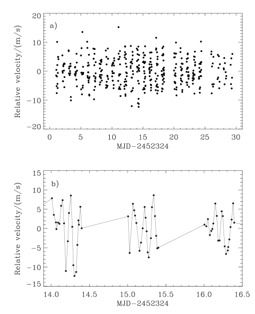
Figure 1: Radial-velocity measurements of $\xi$ Hya. The dispersion reaches $4.6\,{\rm m}\,{\rm s}^{-1}$. a) The whole time string; b) zoom of a small part of the time series.

The $\xi$ Hya observations were made during one full month (2002 February 18 - March 18) with Coralie, the high-resolution fiber-fed echelle spectrograph (Queloz et al. queloz (2001)) mounted on the 1.2-m Swiss telescope at La Silla (ESO, Chile). During the stellar exposures, the spectrum of a thorium lamp carried by a second fiber is simultaneously recorded in order to monitor the spectrograph’s stability and thus to obtain high-precision velocity measurements. The spectra were extracted at the telescope, using the INTER-TACOS (INTERpreter for the Treatment, the Analysis and the COrrelation of Spectra) software package developed by D. Queloz and L. Weber at the Geneva Observatory (Baranne et al. baranne (1996)). The wavelength coverage of these spectra is 3875-6820 Å, recorded on 68 orders. By taking about 2 measurements every hour, a total of 433 optical spectra was collected. The exposure times were typically 180 s and the S/N ratio for all spectra was in the range of 110–230 at 550 nm.

By the use of the optimum-weight procedure (Bouchy et al. bouchy2 (2001)), radial velocities are computed for each night relative to the highest S/N spectrum obtained in the middle of the night. This method requires a Doppler shift that remains small compared to the line-width (smaller than $100\,\rm{m\,s}^{-1}$) (Bouchy & Carrier bouchy3 (2001)). Since the Earth’s motion can introduce a Doppler shift larger than $800\,\rm{m\,s}^{-1}$ during a whole night, each spectrum is first corrected for the Earth’s motion before deriving the radial velocities. This is achieved by shifting all spectra with the Earth’s velocity at the time of observation and by subsequent rebinning, so that the spectra all have the same wavelength values. From each rebinned spectrum a velocity is derived. The mean radial velocity for each night is then subtracted. The resulting velocities are shown in Fig. 1. The rms scatter of the time series is $4.6\,\rm{m\,s}^{-1}$ and is largely due to the oscillations. The mean error on each measurement is $2.3\,\rm{m\,s}^{-1}$.

3 Time-series analysis

Figure 2: Power spectrum for $\xi$ Hya. Modes are clearly present in the range 50–130 $\mu$Hz, corresponding to periods of 2.0-5.5 hours. Panel a) is the power spectrum of the time series using one single spectrum as the reference. Panel b) is for the time series derived using one reference spectrum per night. The insert in Panel b) shows the window function. The frequency scale is made similar to the main plot to facilitate comparison.

The power spectrum of the 433 data points is presented in Fig. 2. In order to show that the excess power in the lower panel in the range 50–130 $\mu$Hz is not due to elimination of power at low frequencies by the reduction procedure, we show a power spectrum in the upper panel where no correction for drift has been applied. Although more noisy the increase in power between 50 $\mu$Hz and 130 $\mu$Hz is also evident in the upper panel. A set of oscillation modes is clearly present, with a power distribution that is remarkably similar to that seen in the Sun and other stars on or near the main sequence, although obviously at much lower frequency. We will show the spectrum displays the characteristic near-uniform spacing of the dominant peaks.

Figure 3: Autocorrelation of the power spectrum for $\xi$ Hya. All points with amplitude $v<1.2$ $\,\rm{m\,s}^{-1}$have been set to zero. The dash-dot-dot-dot vertical lines mark the position of the 11.574 $\mu$Hz daily alias and half of it, and the dash-dot line indicates the peak pointing to a frequency spacing of 6.8 $\mu$Hz.

To characterize this pattern we have calculated the autocorrelation of the power spectrum. In order to eliminate the effect of the noise, we have ignored all points with amplitudes below a given threshhold (1.2 $\,\rm{m\,s}^{-1}$). In Fig. 3 the alias at 1 c/d stands out clearly, but in addition a spacing $\Delta\nu\sim 6.8\ \mu$Hz is present in the power spectrum. This is consistent with the visual impression of a regular pattern present in the the power spectrum (Fig. 2).

The expected velocity amplitude for solar-like oscillations scales as $L/M$ according to Kjeldsen & Bedding (kjeldsen (1995)). Using the stellar parameters from Sect. 4 and a mass of 3.0 $\rm\thinspace M_{\odot}$ (Sect. 4) we find $v_{\rm osc,pred}=4.6\,{\rm m}\,{\rm s}^{-1}.$ The observed amplitudes in Fig. 2 are only about one third of this prediction. Recent calculations by Houdek & Gough (2002), however, indicate that the simple scaling law of Kjeldsen & Bedding (kjeldsen (1995)) does indeed not apply. They predict a velocity amplitude $v=2.1\,{\rm m}\,{\rm s}^{-1}$, slightly higher than the ones observed by us for $\xi$ Hya.

The stochastic nature of solar-like oscillations implies that a timestring of radial velocities cannot be expected to be a set of coherent oscillations and can therefore not be reproduced perfectly by a sum of sinusoidal terms. As a starting point it is nevertheless a good assumption to try to fit the radial-velocity data of $\xi$ Hya by such a set of functions, as the lifetimes are expected to exceed the length of the observing run (Houdek & Gough 2002). We have performed an iterative fit using different methods, among which Period98 (Sperl sperl (1998)) and a procedure by Frandsen et al. (praesepe (2001)). An oscillation with a S/N above 4 is detected at 9 frequencies. When a fit based upon these 9 frequencies is removed from the time series, 5 additional peaks still occur but with a too low S/N to accept them without additional confirmation (hence we do not list them). After removing the 14 frequencies, only a noise spectrum is left. The results for the 9 frequencies are presented in Table 1, where the S/N indicated is calculated from the remaining noise in the amplitude spectrum at the position of each mode. The noise is slightly higher in the range of the modes than at high frequencies, where $\sigma=0.2\,\,\rm{m\,s}^{-1}$. The frequencies of the modes with amplitudes above $1.5\,\rm{m\,s}^{-1}$, i.e., of the five highest-amplitude modes, are unambiguous. Dividing the dataset in two, four out of five modes with S/N $>5.0$ are present in each set. For lower S/N the alias problems lead to a risk that false detections are made. Modes with S/N $<5$ must be considered with some caution. Confirmation of these frequencies is needed by additional observations.

Table 1: Oscillation frequencies detected in the radial velocities of $\xi$ Hya ordered by amplitude. Formal errors of the fit are given in parenthesis as errors of the last digits. The S/N is calculated by dividing the amplitude by the noise in a 10 $\mu$Hz bin in the residual spectrum centered on the frequency of the mode. Frequencies in italic indicate modes where the frequency detection methods disagree on the correct alias. The last column gives the difference between the observed frequency and the frequency derived from Eq. (1).

ID	Frequency		Amplitude	S/N	$\Delta\nu$
	c/d	$\mu$Hz	$\,\rm{m\,s}^{-1}$		$\mu$Hz
F1	5.1344(26)	59.43	1.85(23)	6.6	0.77
F2	6.8366(27)	79.13	1.84(23)	5.8	-0.86
F3	7.4265(29)	85.96	1.76(23)	5.3	-1.14
F4	8.2318(32)	95.28	1.65(23)	5.1	1.07
F5	9.3507(33)	108.22	1.59(23)	6.0	-0.21
F6	8.7399(36)	101.16	1.36(22)	4.5	-0.16
F7	10.0287(43)	116.07	1.25(23)	5.0	0.53
F8	9.0831(44)	105.13	1.24(24)	4.3
F9	8.5339(40)	98.77	1.23(23)	4.1

What is stated above has been verified by the analysis of several sets of simulated data assuming a variety of lifetimes in order to check the validity of the identified modes. The details of such simulations will be published in a subsequent paper.

The first seven modes can be ordered in a sequence of modes, which fits the straight line

$$\nu(n)=1.78+7.11(\pm 0.14)\leavevmode\nobreak\ n$$ (1)

where $n$ is an integer (the order of the mode). Some $n$ values are missing. The maximum deviation from the line is 1.14 $\mu$Hz (Table 1). The regularity seen is similar to the results reported for Arcturus (Merline, 1999) and $\alpha$ UMa (Guenther et al., guenther (2000)). The first seven modes could all be radial modes, although we cannot rule out the possibility of alternating degree $\ell=0$ and $\ell=1$ modes. This, however, is not consistent with the model presented in Sect. 4.

From the present data, we cannot firmly exclude that frequency F8 in Table 1 corresponds to the same mode as F7. The two modes are resolved, but if the damping time is short, they might be different realizations of the same mode.

4 First interpretation

Figure 4: Hertzsprung-Russell diagram with evolutionary tracks for $Z=0.019$ for masses $3.07M_{\odot}$ (solid line), $2.93$ and $3.15M_{\odot}$ (lower and upper dashed lines, respectively). The location of $\xi$ Hya in the diagram is given by the error box.

In order to study the nature of the oscillations detected in $\xi$ Hya, it is necessary to compare the observed frequency spectrum with model predictions, taking into account the constraints on the three observational stellar parameters $T_{\rm eff}$, $L$ and $Z$. We have redetermined the atmospheric parameters and use $T_{\rm eff}=5000\pm 100\$K, $L=61.1\pm 6.2$ $\rm\thinspace L_{\odot}$, $\log g=2.85$, [M/H] = $0.06\pm 0.07$ ($Z=0.019\pm 0.006$) and $v\sin i=1.8\pm 1.0\$$\,\rm{km\,s}^{-1}$. Details of how these values were obtained will be reported in a subsequent paper.

Using the evolution code of Christensen-Dalsgaard (1982), evolutionary tracks were produced, spanning the error box defined by the uncertainties of $T_{\rm eff}$, $L$ and $Z$. The model tracks were computed using the EFF equation of state (Eggleton et al. 1973), OPAL opacities (Iglesias, Rogers & Wilson 1992), Bahcall & Pinsonneault (1992) nuclear cross sections, and the mixing-length formalism (MLT) for convection.

The evolutionary track passing through the observed ($T_{\rm eff}$, $L$) corresponds to a mass of $3.07M_{\odot}$ for $Z=0.019$ (Fig. 4). Oscillation frequencies were calculated for the model in that track closest to the observed location of $\xi$ Hya in the HR diagram. The average separation between radial modes in the range 50–100 $\mu$Hz is $\Delta\nu_{\rm theo}=7.2\,\mu$Hz in agreement with the observational value. The model frequencies fit a linear relation for orders $5<n<17$ or $50<\nu<125\leavevmode\nobreak\ \mu$Hz given by $\nu=7.15+7.14\leavevmode\nobreak\ n$ with absolute values only 1–2 $\mu$Hz from the observed frequencies. The maximum deviation of the model frequencies from the line is $\sim 0.5\leavevmode\nobreak\ \mu$Hz.

Radial modes are expected to dominate the spectrum for giant stars (cf. Dziembowski et al. dziembowski (2001), Fig. 2). Further analysis of the spectrum is beyond the scope of the current discovery paper and will be done in a forthcoming paper, dealing in detail with the issue of modelling and considering also the possibility that $\xi$ Hya could be a core helium burning star with a smaller mass.

5 Conclusions

The main conclusions of this study are as follows. Solar-like oscillations have been firmly discovered in the bright G7III star $\xi$ Hya. The amplitudes of the strongest modes are somewhat below $2\,\rm{m\,s}^{-1}$. The observed frequency distribution of the modes detected (Table 1) is in agreement with theoretically calculated frequencies both in terms of the spacing and the absolute values. The modes with the largest amplitudes can be well matched with radial modes that have an almost equidistant separation around 7.1 $\mu$Hz.

A most important and exciting result of our study is the confirmation of the possibility, suggested by the results reported on $\alpha$ UMa and Arcturus, to observe solar-like oscillations in stars on the red giant branch. This opens the red part of the HR diagram for detailed seismic studies. The latter require an accuracy within the range of current and future ground-based instruments. Such future studies will only be successful if an extremely high stability of the instrument is achieved and if one performs multisite observing campaigns covering several months in order to resolve the frequency spectrum of the oscillations and to eliminate the aliasing problems.

- (1) Bahcall, J. N. & Pinsonneault, M. H. 1992, Rev. Mod. Phys., 64, 885
- (2) Baranne, A., Queloz, D., Mayor, M. et al. 1996, A&AS, 119, 1
- (3) Bedding, T. R., Butler, P. R., Kjeldsen, H., et al. 2001, ApJ, 549, L105
- (4) Bouchy, F. & Carrier, F. 2001, A&A, 374, L5
- (5) Bouchy, F., Pepe, F. & Queloz, D. 2001, A&A, 374, 733
- (6) Buzasi, D., Catanzarite, J., Laher, R. et al. 2000, ApJ, 532, L133
- (7) Carrier, F., Bouchy, F. & Eggenberger, P. 2002, in “Asteroseismology across the HR diagram”, Eds. M.J. Thompson, M.S. Cunha & M.J.P.F.G. Monteiro, Kluwer Academic Publishers, in press
- (8) Christensen-Dalsgaard, J. 1982, MNRAS, 199, 735
- (9) Dziembowski, W. A., Gough, D. O., Houdek, G. & Sienkewicz, R. 2001, MNRAS, 328, 601
- (10) Eggleton, P. P., Faulkner, J. & Flannery, B. P. 1973, A&A, 23, 325
- (11) Frandsen, S., Pigulski, A., Nuspl, J. et al. 2001, A&A, 376, 175
- (12) Guenther, D. B., Demarque, P., Buzasi, D. et al. 2000, ApJ, 520, L45
- (13) Houdek, G. & Gough, D. O. 2002, MNRAS, submitted
- (14) Iglesias, C. A., Rogers, F. J. & Wilson, B. G. 1992, ApJ, 397, 717
- (15) Kjeldsen, H. & Bedding, T. R 1995, A&A, 293, 87
- (16) Martic, M., Schmitt, J., Lebrun, J. et al. 1999, A&A, 351, 993
- (17) Merline, W.J. 1999, in “Precise Stellar Radial Velocities”, IAU Coll. 170, Eds. J.B. Hearnshaw & C.D. Scarfe, ASP Conf. Ser. Vol. 185, 187
- (18) Queloz, D., Mayor, M., Ubry, S. et al. 2001, The Messenger, 105, 1
- (19) Retter, A., Bedding, T.R., Buzasi, D. & Kjeldsen, H. 2002, in “Asteroseismology across the HR diagram”, Eds. M.J. Thompson, M.S. Cunha & M.J.P.F.G. Monteiro, Kluwer Academic Publishers, in press (Astro-ph/0208518)
- (20) Sperl M. 1998, Comm. in Asteroseismology (Vienna), 111, 1