GRAVITATIONAL LENSING AT MILLIMETER WAVELENGTHS

Summary.

The study of gas and dust at high redshift gives an unbiased view of star formation in obscured objects as well as the chemical evolution history of galaxies. With today’s millimeter and submillimeter instruments observers use gravitational lensing mostly as a tool to boost the sensitivity when observing distant objects. This is evident through the dominance of gravitationally lensed objects among those detected in CO rotational lines at $z>1$. It is also evident in the use of lensing magnification by galaxy clusters in order to reach faint submm/mm continuum sources. There are, however, a few cases where millimeter lines have been directly involved in understanding lensing configurations. Future mm/submm instruments, such as the ALMA interferometer, will have both the sensitivity and the angular resolution to allow detailed observations of gravitational lenses. The almost constant sensitivity to dust emission over the redshift range $z\approx 1-10$ means that the likelihood for strong lensing of dust continuum sources is much higher than for optically selected sources. A large number of new strong lenses are therefore likely to be discovered with ALMA, allowing a direct assessment of cosmological parameters through lens statistics. Combined with an angular resolution $<0\hbox{$\,.\!\!^{\prime\prime}$}1$, ALMA will also be efficient for probing the gravitational potential of galaxy clusters, where we will be able to study both the sources and the lenses themselves, free of obscuration and extinction corrections, derive rotation curves for the lenses, their orientation and, thus, greatly constrain lens models.

1 Introduction

Rapid progress in the development of millimeter astronomical facilities, such as the increase of antennae sizes and/or of the number of array elements, or as the continuing improvement in the sensitivity of detectors, have now made it possible to explore the high redshift universe in this window and therefore to exploit the potentialities of gravitational lensing effects.

Why is it so important to explore this wavelength domain? In one short statement: the presence of cold dust and of molecular material can be traced in this window and both components witness the formation of heavy elements. If they are detected in galaxies at high redshifts, they allow us to probe star formation in the early universe. They reveal as well processes related to the startup of active galactic nuclei (AGN) and signal the presence of massive black-holes. Large amounts of molecular gas are encountered in the close environment of the central engine in AGN. This material is often regarded as the fuel which allows to activate the AGN. An evolutionary scenario would then connect IR-luminous galaxies rich in molecular material and with intense star formation to the formation/feeding of massive black holes.

Several fundamental questions are therefore underlying the search for dust and molecular gas at high redshift: the redshift of galaxy formation? the chemical evolution of the universe with time? the evolution of the dust content in the universe at early ages? the epoch and the scenario of the formation of massive black holes? the startup and evolution of AGN activity? Do we have already some clues to answer these questions? The most powerful AGNs, quasars, are now detected up to redshift around 6.5, and galaxies up to redshift 6. So we know that in this redshift range the universe already hosted galaxies and massive black holes and that its metal content was substantial since the spectra of high redshift AGNs are very similar to those of low redshift AGNs. Yet, only a few objects are known at these high redshifts and this may provide a biased view. It is therefore mandatory to enlarge the sample and of course, the goal is also to push the redshift limit.

Pushing the redshift limit also means that we are investigating sources with lower and lower flux density. This can be achieved through technical improvements, using larger collectors and better detectors. The ALMA project is showing the way. Another manner is to take advantage of the effects induced by gravitational lensing (for a review of its theoretical basis, see the comprehensive book by Schneider et al. schneider92 ). Firstly, image magnification allows us to detect more distant sources of cold dust and molecular gas of a given intrinsic luminosity, or to detect at a given redshift sources of fainter intrinsic luminosity. The latter in particular is important for good determinations of luminosity functions. Secondly, differential magnification effects can be used as an elegant tool to probe the size of molecular and dusty structures in the lensed source, as long as the lensing system provides the appropriate geometry. In this case, it is imperative to have an excellent model of the lensing system, as any structural information about the source itself for example is recovered by tracing the image back through the lensing system. Both aspects will be discussed at length in this paper. In some cases molecular absorption lines allow us to obtain information about the lensing galaxy itself.

Apart from hydrogen and helium, carbon and oxygen are the heavy elements with highest abundance in the universe. Therefore, the CO molecule is the most suitable candidate for the detection of molecular gas in emission at high redshift. The CO molecules can be detected directly through their thermal line emission in the source or as silhouetted absorbers along the line of sight to a background source. The latter may occur for example for the lensing galaxy. Several other molecules have been detected at high redshift, HCO⁺, HCN, H₂CO…, while dust is detected essentially through its thermal emission.

We provide in Sect. 2 an overview of the CO line emission and of the high redshift CO sources detected so far. The role played by gravitational lensing in studying CO sources at high redshift is highlighted. In Sect. 3 we review molecular absorption and the importance of such measurements to investigate the properties of the lensing galaxies. Sect. 4 introduces the dust continuum emission and the use of differential magnification effects which can be made to probe the dust content of the lensed objects. Three cases particularly well studied are discussed in detail in Sect. 5. In Sect. 6 existing lens models for PKS1830-211 are reviewed and a new one introduced. Finally, in Sect. 7 the future of this type of investigations is presented in the perspective of new instrumental developments in general and of ALMA in particular.

2 MOLECULAR EMISSION

The goal of this section is primarily to highlight the benefits of exploiting gravitational lensing effects in the millimeter range, that is in CO line emission. Therefore, after some brief comments on the pioneering observations of low redshift sources, we shall concentrate on the results obtained on high redshift sources. This section deals essentially with the CO line emission, while the following sections will discuss molecular absorption lines and dust thermal emission.

Detection and measurements of the ¹²CO rotational transitions in Galactic and extragalactic sources have had a great impact on the development of astrochemistry. The J=1-0 CO transition is excited by collisions with H₂ molecules, even in clouds at low kinetic temperature. The low-J transitions are in general optically thick, the opacity being determined observationally by the relative intensity of the corresponding ¹³CO transition. On the contrary, the high-J transitions are optically thin. Therefore, it is quite interesting to perform multi-transition studies to ascertain in a more secure fashion the physical conditions, temperature and density, in the emitting molecular material. This is particularly true in the case of very dense molecular material exposed to intense radiation fields, like in the environment of an AGN or in powerful star forming regions. The conversion factor which is used to derive the total mass of molecular material from the observed L_CO, is also highly dependent on the physical conditions in the molecular material. It has been determined to be 4.6 M_⊙ (K km s^-1 pc²)^-1 in standard Milky Way clouds solomon87 . Recently it has been shown that lower values of the conversion factor (by up to a factor 10) should be used in the case of dense and warm material as usually encountered in a molecular torus around an AGN downes98 .

2.1 Low- and intermediate redshift galaxies

Following far-infrared (FIR) observations by IRAS, an important population of IR-luminous (dust-rich) galaxies was found. This was the starting point for investigating as well their molecular content, using the millimeter facilities available in the late 80’s. A number of IR-luminous galaxies and AGNs were detected, mostly in the CO(1-0) transition and the field develop quickly. Regarding low redshift sources, let us briefly mention the detection of AGNs such as Mrk 231 sanders87 , Mrk 1014 sanders88 , I Zw 1 barvainis89 and of some low redshift quasars sanders89 alloin92 or radio galaxies phillips87 mirabel89 mazzarella93 . At moderate redshift, CO was detected in the radio galaxy 3C48 ($z=0.369$) scoville93 . This search is continuing through e.g. the Caltech CO high and low redshift radio galaxy survey evans99 .

On the side of CO sources at high redshift (z$>$2), the first object detected was IRAS 10214+4724 brown92 solomon92 . All along the 90’s, millimeter dishes and interferometer arrays in service were pushed to their limits in searching for other candidates, selected for example upon the strength of their submillimeter flux. A large amount of observing time was dedicated to such programs at the OVRO, BIMA, Nobeyama and IRAM facilities. At face value, the success rate in detecting high redshift CO sources has been modest. One reason for this is the uncertainty in the precise redshift of the emitting molecular gas under search, while the backends of the instruments are narrow in comparison to the redshift range to be explored. Another reason is of course the limited sensitivity of existing instruments. Only the most luminous and most gas-rich systems can be detected. The situation should improve with new facilities such as ALMA (See Sect. 7.1). Sources detected so far are detailed below, in order of increasing redshift.

Table 1: Galaxies at z$>$1 with molecular emission (January 2002)

Name	z		$M_{\rm H_{2}}$	$M_{\rm d}$/M⊙	$L_{\rm FIR}$/L⊙	Grav. lens	Ref.
BR1202$-$0725	4.69		$6\times 10^{10}$	$2\times 10^{8}$	$\sim 1\times 10^{12}$	?	ohta96 , omont96
BR0952$-$0115	4.43		$3\times 10^{9}$	$3\times 10^{7}$	$\sim 1\times 10^{12}$	YES	guilloteau99
BRI1335$-$0414	4.41		$1\times 10^{11}$	continuum det.	—	NO?	guilloteau97
PSS2322+1944	4.12		$3\times 10^{11}$	$1\times 10^{9}$	—	?	cox02
APM08279+5255	3.91		$2\times 10^{9}$	$1\times 10^{7}$	$\sim 8\times 10^{13}$	YES	downes99b
4C60.07	3.79		$8\times 10^{10}$	$2\times 10^{8}$	$\sim 2\times 10^{13}$	NO	papadopoulos00
6C1909$+$722	3.53		$4\times 10^{10}$	$2\times 10^{8}$	$\sim 2\times 10^{13}$	NO	papadopoulos00
MG0751+2716	3.20		$8\times 10^{10}$	—	—	YES	barvainis02
SMM02399$-$0136	2.81		$8\times 10^{10}$	continuum det.	$\sim 1\times 10^{13}$	YES	frayer98
MG0414$+$0534	2.64		$5\times 10^{10}$	continuum det.	—	YES	barvainis98
SMM14011$+$0252	2.56		$5\times 10^{10}$	continuum det.	$\sim 3\times 10^{12}$	YES	frayer99
H1413$+$117	2.56		$2\times 10^{9}$	$1\times 10^{8}$	$\sim 2\times 10^{12}$	YES	barvainis94
53W002	2.39		$1\times 10^{10}$	weak continuum	—	NO	scoville97
F10214$+$4724	2.28		$2\times 10^{10}$	$9\times 10^{8}$	$\sim 7\times 10^{12}$	YES	brown92
HR 10	1.44		$7\times 10^{10}$	$2\times 10^{8}$	$\sim 9\times 10^{11}$	NO	andreani00

Masses and fluxes corrected for gravitational magnification (approx.)
 

2.2 High redshift galaxies

The first source discovered, IRAS 10214+4724, at $z=2.285$, has been detected in CO(3-2), CO(4-3) and CO(6-5) brown92 solomon92 . A report on the detection of CO(1-0) tsuboi94 remains to be confirmed. The source is a gravitationally lensed ultraluminous IR-galaxy broadhurst95 downes95 . The magnification factor is found to be around 10 for the CO source which has an intrinsic radius of 400 pc. Conversely, the far-IR emission detected in this object is magnified 13 times and arises from a source with radius 250 pc, while the mid-IR is magnified 50 times and arises from a source with radius 40 pc. After correcting for magnification, and using a conversion factor L${}^{\prime}_{\rm CO}$ to M(H₂) of 4 M_⊙ (K km s^-1 pc²)^-1 radford91 , the molecular gas mass is found to be $2\times 10^{10}$ M_⊙, in agreement with the estimated dynamical mass $3\times 10^{10}$ M_⊙. As noted above however, such a value for the conversion factor, obtained from CO(1-0) observations of Galactic molecular clouds, might not be applicable in the case of warmer and denser molecular material. A value for the conversion factor which is 5 times lower than the standard has been found in a study of extreme starbursts in IR-luminous galaxies downes98 . Hence, the mass value quoted above should regarded as an upper limit to the mass of the molecular gas in IRAS 10214+472. Still pending is the question of the CO line emission share between a hidden AGN and a starburst in the 400 pc region surrounding the AGN. We notice also that the large extension (3 to 12 kpc) in CO emission reported by scoville95 has not been confirmed by the IRAM interferometer data downes95 .

One interesting case is that of the radio galaxy 53W002 at $z=2.394$, located at the center of a group of $\sim$20 Lyman-$\alpha$ emitters. A possible detection of the CO(1-0) line at Nobeyama was reported in yamada95 , although not yet confirmed by others. The first detection in CO(3-2) by OVRO scoville97 suggested a large extension (30 kpc) and the existence of a velocity gradient. None of these features has been confirmed by an IRAM interferometer data set with higher signal to noise ratio alloin00 . From an astrometric analysis it is found that the 8.4 GHz and CO source are coincident, at a location consistent with that of the optical/UV continuum source. The most likely origin of the molecular emission is therefore from the close environment of the AGN. One should notice that 53W002 is definitely not a gravitationally lensed source. Using a conversion factor L${}^{\prime}_{\rm CO}$ to M(H₂) in the range 0.4 - 0.8 M_⊙ (K km s^-1 pc²)^-1, more appropriate for dense and warm molecular gas around an AGN barvainis97 , the resultant molecular gas mass is found to be in the range $(0.6-1.0)\times 10^{10}$ M_⊙.

The Cloverleaf, H1413+117 is a well known gravitationally lensed Broad Absorption Line (BAL) quasar at $z=2.558$ magain88 . Its CO(3-2) transition was first observed with the IRAM 30m dish barvainis94 and then with BIMA wilner95 . Later, the CO(4-3), CO(5-4) and CO(7-6) transitions have been detected, together with HCN(4-3) and a fine-structure line of CI. From a detailed analysis of these transitions, the molecular gas was found to be warm and dense barvainis97 with a low conversion factor of 0.4 M_⊙ (K km s^-1 pc²)^-1. High resolution maps in the CO(7-6) transition were obtained with OVRO yun97 and with the IRAM interferometer alloin97 kneib98a . The IRAM map has the best resolution and signal to noise ratio. Comparing with the HST images and exploiting differential gravitational effects, the CO(7-6) map allowed a derivation of both the the size and the kinematics of the molecular/dusty torus around the quasar central engine kneib98a (for further details see Sect. 5.2). After correcting for the amplification factor (30 according to the model used for the lensing system), and using the mean conversion factor 0.6 M_⊙ (K km s^-1 pc²)^-1 (derived by Barvainis et al. barvainis97 ), the derived mass of molecular gas M(H₂) is $2\times 10^{9}$ M_⊙, in agreement with the dynamical mass of $8\times 10^{8}$ M_⊙.

The source SMM 14011+0252 was observed with OVRO in CO(3-2) at $z=2.565$ frayer99 , following its discovery as a strong submillimeter source detected in the course a survey of rich lensing clusters smail98b . Correcting for an amplification factor of 2.75 and using a conversion factor of 4 M_⊙ (K km s^-1 pc²)^-1, the mass of molecular gas turns out to be $5\times 10^{10}$ M_⊙, while the dynamical mass is found to be larger than $1.5\times 10^{10}$ M_⊙. The CO emission is extended on scales of $\sim$10 kpc and associated with likewise extended radio continuum emission ivison01 . Optical and near-infrared (NIR) imaging shows two objects (designated J1 and J2), separated by 2$\,.\!\!^{\prime\prime}$1 ivison00 . Both the molecular gas and the radio continuum, however, have their strongest emission $\sim$1^′′ north of the J1/J2 components and are extended between J1 and J2. This suggests that the optical/NIR emission comes from two ‘windows’ in the obscuring molecular gas and dust and that J1/J2 represent emission from a coherent large galaxy. The extended nature of the radio continuum, the lack of X-ray emission fabian00 and the lack of optical broad emission lines (Wiklind et al. 2002 in prep) suggest that only star formation powers the large FIR luminosity. Assuming a Salpeter initial mass function and correcting for the gravitational magnification, the FIR luminosity indicates a star formation rate exceeding 10³ M_⊙ yr^-1.

The gravitationally lensed quasar MG 0414+0534 was observed with the IRAM interferometer in the CO(3-2) transition at $z=2.639$ barvainis98 . The lensed nature of this system is known from a 5 GHz map hewitt92 . It displays four quasar-spots separated at most by $\sim 2^{\prime\prime}$. The beam of the IRAM data (2$\,.\!\!^{\prime\prime}$0 $\times$ 0$\,.\!\!^{\prime\prime}$9) does not allow to separate the components in the CO(3-2) velocity-integrated map. However, by fitting the UV data directly, it has been possible to resolve the combined A components (A1+A2) from component B and to get separate CO(3-2) spectra. The relative strength A:B in the 5 GHz radio continuum is 5:1. The millimeter continuum rather shows a ratio 7:1 and differences are seen between the A and B CO(3-2) spectra, suggesting that differential magnification effects may be at work. The magnification factor is unknown: hence only an upper limit can be derived for the molecular gas mass. Assuming in addition a conservative conversion factor of 4 M_⊙ (K km s^-1 pc²)^-1, the upper limit found for M(H₂) is $2.2\times 10^{11}$ M_⊙. This figure is below the upper limit derived for the dynamical mass, $9\times 10^{11}$ M_⊙.

Another source detected first through submillimeter observations is SMM 02399-0136 ivison98 . It is known to be gravitationally amplified by a foreground cluster of galaxies, the amplification factor being 2.5. This source has been detected with OVRO in the CO(3-2) transition at $z=2.808$ frayer98 . The mass of molecular gas deduced in this object, correcting for a 2.5 amplification factor and using the conversion factor applicable to Galactic clouds, 4 M_⊙ (K km s^-1 pc²)^-1, is $8\times 10^{10}$ M_⊙. From the upper limit on the apparent size of the CO emitting source (5^′′) and the width of the CO line (710 km s^-1), an upper limit to the mass of molecular gas of $1.5\times 10^{10}$ M_⊙ can be derived frayer98 . The SCUBA results indicate that SMM 02399-0136 is an IR-hyperluminous galaxy. On the other hand, optical data shows clearly than it hosts as well a dust-enshrouded AGN ivison98 . A precise share of CO emission between the two components remains to be investigated.

In the course of a systematic CO emission survey of gravitationally lensed sources with the IRAM interferometer barvainis02 , the source MG 0751+2716 has been detected in the CO(4-3) transition at $z=3.200$. This source was first discovered to be a gravitationally lensed quasar, from VLA maps lehar97 . It shows four quasar-spots with maximum separation of 0$\,.\!\!^{\prime\prime}$9. The lensing galaxy, which provides the image geometrical configuration, is part of a group of galaxies adding another shear to the lens-system tonry99 . The lensing system remains to be modeled in detail. Therefore, the amplification factor is not known. However, given the observed strength of the CO line emission it should be large. Assuming that the CO emission in this source is mostly from the close environment of the AGN, we consider a conversion factor in the range 0.4 to 1 M_⊙ (K km s^-1 pc²)^-1. The corresponding upper limit (no correction applied for the unknown amplification factor) for the mass of molecular gas is in the range $8\times 10^{10}$ to $2\times 10^{11}$ M_⊙ barvainis02 .

The distant powerful radio galaxy 6C 1909+722 has been detected in the CO(4-3) line at $z=3.53$, with the IRAM interferometer, and in dust submillimeter emission using SCUBA papadopoulos00 . It is unlikely to be a gravitationally lensed object. Hence, the derived mass of molecular material is quite large, even assuming a conservative value for the conversion factor (about one fifth the value derived from Galactic molecular clouds). It is found to be in the range $(0.5-1.0)\times 10^{11}$ M_⊙.

Another possibly unlensed powerful radio galaxy 4C 60.07, has been detected in the CO(4-3) line emission at $z=3.79$ at IRAM, and in dust thermal emission at submillimeter wavelengths with SCUBA and at millimeter wavelengths at IRAM papadopoulos00 . Remarkably, the CO line emission extends over 30 kpc and breaks into two components: one corresponding to the AGN (radio core) and a second one which is rather related to a major episode of star formation. This state of merging is speculatively interpreted as the formative stage of an elliptical host around the residing AGN. Again, the molecular mass is found to be quite large, around $10^{11}$ M_⊙.

The gravitationally lensed BAL quasar, APM 08279+5255, has been detected in the CO(4-3) and CO(9-8) transitions at $z=3.911$, with the IRAM interferometer downes99b . The CO line ratio points towards warm and dense molecular gas. Thermal emission from the dust component is also measured. Both the molecular and dust luminosities appear to be very high. Gravitational amplification is therefore suspected and has subsequently been confirmed through the detection of three optical/NIR components ledoux98 egami00 (see also Sect. 5.1 and Fig. 13). The magnification factors for the molecular gas and dust where estimated downes99b . After correcting for these factors, the dust mass is found to be in the range $(1-7)\times 10^{7}$ M_⊙, and the molecular gas mass in the range $(1-6)\times 10^{9}$ M_⊙. In this interpretation, the molecular/dusty component is in the form of a nuclear disk with radius 90-270 pc orbiting the central engine of the BAL quasar. This source looks therefore quite similar to the Cloverleaf. Recently, however, extended low-excitation CO emission (the J=1-0 and J=2-1 transitions) have been detected using the VLA papadopoulos01 . This extended emission is likely to be associated with a cooler molecular component than the CO(9-8) emission.

Finally, let’s discuss the four sources detected so far at z larger than 4:

PSS 2322+1944 The radio quiet quasar PSS 2322+1944 has recently been detected in the CO(5-4) and CO(4-3) transitions at a redshift of $z=4.12$ with the IRAM interferometer cox02 . The velocity-integrated CO line fluxes are $3.74\pm 0.56$ and $\rm 4.24\pm 0.33$ Jy km s^-1, with a linewidth $\approx 330$ km s^-1. The 1.35 mm (250$\rm\mu m$ restwavelength) dust continuum flux density is 7.5 mJy, in agreement with previous measurements at 1.25 mm at the IRAM 30m telescope omont01 , and corresponds to a dust mass of $\approx 10^{9}$ M_⊙. With the present angular resolution of the observations, no evidence for extended emission has been found yet. The implied gas mass is estimated to be $\rm\approx 3\times 10^{11}$ M_⊙, using a conversion factor of $\rm 4.6$ M_⊙ K km s^-1 pc². The properties of PSS 2322+1944 are described in detail in cox02 .

BRI 1335-0415 BRI 1335-0415 was detected in the CO(5-4) transition with the IRAM interferometer at $z=4.407$ guilloteau97 . The source does not exhibit a noticeable extension neither in the 1.35mm continuum nor in the CO line emission. In addition, there is no obvious sign of gravitational lensing on the line-of-sight to this source. The authors have derived a very large mass of molecular gas, close to 10¹¹ M_⊙. Even with a conversion factor 3 times smaller, more appropriate for this type of object, the mass remains a few 10¹⁰ M_⊙.

BR 0952-0115 The gravitationally lensed radio quiet quasar BR 0952-0115 has been detected in CO(5-4) with IRAM facilities at $z=4.43$ guilloteau99 . A tentative estimate of the mass of molecular material M(H₂) is $3\times 10^{9}$ M_⊙. Note however that a more precise model of the lens has still to be worked out.

BR 1202-01215 BR 1202-01215 is the most distant source detected in CO. It has been reported in the CO(5-4) transition observed with the Nobeyama array ohta96 , and in the CO(4-3), CO(5-4) and CO(7-6) lines observed with IRAM facilities omont96 . The CO maps show two separate sources on the sky: one is coincident with the optical quasar (for this source CO(5-4) provides $z=4.695$), while the other is located 4” to the North-West, where no optical counterpart is found (for this source CO(5-4) provides $z=4.692$). At this redshift the 4^′′ extension corresponds to a de-projected distance of 12-30 kpc. It is uncertain whether this object is gravitationally lensed or not. Is the North-West source a second image of the quasar? There are hints that this might be the case as a strong gravitational shear has been measured in the field (Fort and D’Odorico, private communication). Else, each of two separate sources ought to have its own heating source, AGN or starburst. Assuming no gravitational boost and using a conversion factor of 4 M_⊙ (K km s^-1 pc²)^-1, the mass of molecular gas is quoted to be $6\times 10^{10}$ M_⊙.

A summary of the sources properties is provided in Table 1. This quick compilation of high redshift CO sources has prompted a number of key-issues:

(i) A major difficulty in detecting high redshift CO sources is the lack of precision in our guess for the redshift of the molecular gas. The instantaneous frequency coverage of current backends requires that the redshift is known a-priori with a precision of a few percent. Why is this condition hard to fulfill? The molecular gas emission in distant objects can arise from the close environment of an AGN. Yet, published redshifts for distant AGN are mostly measured from emission lines of highly ionized species which can be strongly affected by winds. Indeed velocity offsets of up to 2500 km s^-1 have been observed between the CO lines and the blue-shifted CIV line for example (e.g. downes99b ). Hopefully, this limitation will be overcome with the next generation of backends.

(ii) An uncertain part in the interpretation of the observed CO line intensities lies with the physical state of the molecular gas and the conversion factor L${}^{\prime}_{\rm CO}$ to M(H₂) to be applied in the case of high redshift sources. When several CO transitions are observed (such as for IRAS10214+4724, H1413+117, APM 08279+5255 and BR 1202-0725), the physical conditions of the molecular gas can be analyzed, pointing towards warm (T$\sim$100 K), dense (a few 10³ cm^-3) and moderately optically thick material. Such conditions could very well characterize molecular gas in the proximity of an AGN. Conversely, the conditions of the molecular gas in an extended starburst may be more similar to those encountered in Galactic molecular clouds. The conversion factor depends on the physical conditions of the molecular gas. It ranges from a value of 4 M_⊙ (K km s^-1 pc²)^-1 in Galactic clouds radford91 , to 1 M_⊙ (K km s^-1 pc²)^-1 in IR-ultraluminous galaxies downes98 and possibly 0.4 M_⊙ (K km s^-1 pc²)^-1 in the surroundings of an AGN barvainis97 . Therefore, it would be important to have some clues about the share AGN/starburst in the heating mechanism for high redshift CO sources. In that respect, the CO line width and the compactness of the source may bring some pieces of information.

(iii) Finally, the outmost efforts should be made to find out whether a source is gravitationally lensed or not, before the claim for the presence of a huge amount of molecular gas (10¹¹ M_⊙) can be taken as a starting point for modeling. Weak shear from an intervening galaxy cluster, like in the cases of SMM 14011+0252 and SMM 02399-0136, induces a mild magnification factor in the range 2-3. Strong shear (possibly combined with weak shear), induces magnification factors of up to 30! This would decrease by one order of magnitude the mass of molecular gas derived. If, at the same time, the applicable conversion factor is on the low side of its possible values range, a reduction of the actual molecular gas mass by another order of magnitude would apply.

In conclusion, it is important to search for other high redshift CO sources and, at the same time, to investigate carefully the nature of their environment/line-of-sight and the physical conditions in their molecular gas.

3 MOLECULAR ABSORPTION LINES

Another method to study molecular gas at high redshift is to observe molecular rotational lines in absorption rather than emission. Whereas emission is biased in favor of warm and dense molecular gas, tracing regions of active high mass star formation, molecular absorption lines trace excitationally cold gas. This is important since a large part of the molecular gas mass may reside in regions far away from massive star formation and therefore remain largely unobserved in emission.

Molecular absorption occurs whenever the line of sight to a background quasar passes through a sufficiently dense molecular cloud. In contrast to optical absorption lines seen towards most high redshift QSOs, molecular absorption is invariably associated with galaxies, either in the host galaxy of the continuum source or along the line of sight. In nearby galaxies molecular gas is strongly concentrated to the central regions, making the likelihood for absorption largest whenever the line of sight passes close to the center of an intervening galaxy. This, of course, means that molecular absorption in intervening galaxies is likely to be associated with gravitational lensing, and vice versa. Indeed, the only known systems of intervening absorption (B0218+357 and PKS1830-211) are gravitationally lensed and the absorption probes molecular gas in the lensing galaxy. Molecular absorption lines can thus be used to study the neutral and dense interstellar medium in lenses. At the present the sample of lens galaxies probed by molecular absorption lines is limited, but with the advent of a new sensitive interferometer instrument like ALMA, the number of potential candidate systems will increase substantially and make it possible to probe the molecular interstellar medium in the lens galaxies in some detail. Moreover, the molecular absorption lines provide unique kinematical information which is valuable when constructing a model of the lensed system.

3.1 Detectability

As mentioned above, molecular absorption traces a different gas component then emission lines. For optically thin emission the integrated signal $I_{\rm CO}$ is

$$I_{\rm CO}=\int{T_{\rm a}\,dv}\ \propto\ N_{\rm tot}\,T^{-1}\,e^{-E_{\rm u}/kT}\,(e^{{\rm h}\nu/{\rm k}T}-1)\left[J(T)-J(T_{\rm bg})\right]\ \ ,$$

where $N_{\rm tot}$ is the total column density of a given molecular species, $E_{\rm u}$ the upper energy level of a transition with $\Delta E=h\nu$, $T_{\rm bg}$ is the local temperature of the Cosmic Microwave Background Radiation (CMBR) and $J(T)=(h\nu/k)(e^{h\nu/kT}-1)^{-1}$. When $T\rightarrow T_{\rm bg}$ all the molecules reside in the ground rotational state $J=0$ and the signal disappears. For molecular absorption the observable is the velocity integrated opacity $I_{\tau_{\nu}}$:

$$I_{\tau_{\nu}}=\int{\tau_{\nu}\,dv}\ \propto\ N_{\rm tot}\,T^{-1}\,\mu_{0}^{2}\,e^{-E_{l}/kT}\,(1-e^{-h\nu/kT})\ \ ,$$

where $N_{\rm tot}$ is again the total column density of a given molecular species, while $E_{l}$ is now the lower energy level and $\mu_{0}$ is the permanent dipole moment of the molecule. For the ground transition, $E_{l}=0$, $I_{\tau_{\nu}}\propto N_{\rm tot}\,T^{-1}\,\mu_{0}^{2}\,(1-e^{-h\nu/kT})\approx(h\nu/k)\,N_{\rm tot}\,\mu_{0}^{2}\,T^{-2}$. In contrast to emission lines, the observed integrated opacity increases as the temperature $T$ decreases.

Molecules are generally excited through collisions with molecular hydrogen H₂. The excitation temperature, $T_{\rm x}$, therefore depends strongly on the H₂ density. The collisional excitation is balanced by radiative decay and a steady-state situation with $T_{\rm x}=T_{\rm k}$ requires a certain critical H₂ density. For CO, which has a small permanent dipole moment $\mu_{0}$, the critical density is rather low, $4\times 10^{4}$ cm^-3, while molecules with higher dipole moments require higher densities. For instance, HCO⁺ which has a dipole moment more than 30 times larger than that of CO, the critical density is $2\times 10^{7}$ cm^-3.

The strong dependence of the opacity on the permanent dipole moment means that absorption preferentially probes low excitation gas, i.e. a cold and/or diffuse molecular gas component. If multiple gas components are present in the line of sight, with equal column densities but characterized by different excitation temperatures, absorption will be most sensitive to the gas component with the lowest temperature. The dependence of the opacity on the permanent dipole moments also means that molecules much less abundant than CO can be as easily detectable. For instance, HCO⁺ has an abundance which is of the order $5\times 10^{-4}$ that of CO, yet it is as easy, or easier, to detect in absorption as CO. This is illustrated in Fig. 1, where the observed opacity of the CO(1-0) and HCO⁺(2-1) transitions at $z=0.25$ are compared. In this particular case, the HCO⁺ line has a higher opacity than the CO line.

3.2 Observables

Analysis of the molecular absorption lines gives important information about both the physical and chemical properties of the interstellar medium. This can have implications for identifying the type of galaxy causing the absorption and, in some cases, help to identify the morphological type of lenses. In this section a short description of the analysis that can be done is presented. A more detailed description can be found in the references given in the text.

Optical depth.

The observed continuum temperature, $T_{\rm c}$, away from an absorption line can be expressed as $T_{\rm c}=f_{\rm s}J(T_{\rm b})$, where $f_{\rm s}$ is the beam filling factor of the region emitting continuum radiation, $T_{\rm b}$ is the brightness temperature of the background source and $J(T)=(h\nu/k)/[1-\exp(-h\nu/kT)]$ (e.g. wiklind97 ). The spatial extent of the region emitting continuum radiation at millimeter wavelengths is unknown but is certain to be smaller than at longer wavelengths. The BL Lac 3C446 has been observed with mm-VLBI and has a size $<30\,\mu$arcseconds lerner93 . Since the angular size of a single dish telescope beam at millimeter wavelengths is typically $10^{\prime\prime}-25^{\prime\prime}$, the brightness temperature of the background source, $T_{\rm b}$, is at least $10^{9}\times T_{\rm c}$. This means that the local excitation temperature of the molecular gas is of no significance when deriving the opacity. The excitation does enter, however, when deriving column densities.

Excitation temperature and column density.

The excitation temperature, $T_{\rm x}$, relates the relative population of two energy levels of a molecule as: $\frac{n_{2}}{n_{1}}=\frac{g_{2}}{g_{1}}\ e^{-h\nu_{21}/kT_{\rm x}}$, where $g_{i}$ is the statistical weight for level $i$ and $h\nu_{21}$ is the energy difference between two rotational levels. In order to derive $T_{\rm x}$ we must link the fractional population in level $i$ to the total abundance. This is done by invoking the weak LTE-approximation. We can then use the partition function $Q(T_{\rm x})=\sum_{J=0}^{\infty}g_{J}\,e^{-E_{J}/kT_{\rm x}}$ to express the total column density, $N_{\rm tot}$, as

$$N_{\rm tot} = {8\pi\over c^{3}}{\nu^{3}\over g_{J}A_{J,J+1}}f(T_{\rm x})\ \int\tau_{\nu}dV\ ,$$ (1)

(2)

$$f(T_{\rm x}) = {Q(T_{\rm x})e^{E_{J}/kT_{\rm x}}\over 1-e^{-h\nu/kT_{\rm x}}}\ ,$$ (3)

where $\int\tau_{\nu}dV$ is the observed optical depth integrated over the line for a given transition, $g_{\rm J}=2J+3$ for a transition $J\rightarrow J+1$, and $E_{\rm J}$ is the energy of the rotational level $J$. By taking the ratio of two observed transitions from the same molecule, the excitation temperature can be derived. The strong frequency dependence of the column density in Eq. 1 is only apparent since the Einstein coefficient, $A_{J,J+1}$, is proportional to $\nu^{3}$.

Table 2: Properties of molecular absorption line systems.

Source	z${}_{\rm a}^{(a)}$	z${}_{\rm e}^{(b)}$	$N_{\rm CO}$	$N_{\rm H_{2}}$	$N_{\rm HI}^{(c)}$	A${}_{\rm V}^{\prime\ (d)}$	$N_{\rm HI}/N_{H_{2}}$
			cm-2	cm-2	cm-2
Cen A	0.00184	0.0018	$1.0\times 10^{16}$	$2.0\times 10^{20}$	$1\times 10^{20}$	50	0.5
PKS1413+357	0.24671	0.247	$2.3\times 10^{16}$	$4.6\times 10^{20}$	$1.3\times 10^{21}$	2.0	2.8
B3 1504+377A	0.67335	0.673	$6.0\times 10^{16}$	$1.2\times 10^{21}$	$2.4\times 10^{21}$	5.0	2.0
B3 1504+377B	0.67150	0.673	$2.6\times 10^{16}$	$5.2\times 10^{20}$	$<7\times 10^{20}$	$<$2	$<$1.4
B 0218+357	0.68466	0.94	$2.0\times 10^{19}$	$4.0\times 10^{23}$	$4.0\times 10^{20}$	850	$1\times 10^{-3}$
PKS1830–211A	0.88582	2.507	$2.0\times 10^{18}$	$4.0\times 10^{22}$	$5.0\times 10^{20}$	100	$1\times 10^{-2}$
PKS1830–211B	0.88489	2.507	$1.0\times 10^{16\ (e)}$	$2.0\times 10^{20}$	$1.0\times 10^{21}$	1.8	5.0
PKS1830–211C	0.19267	2.507	$<6\times 10^{15}$	$<1\times 10^{20}$	$2.5\times 10^{20}$	$<$0.2	$>$2.5

$(a)$ Redshift of absorption line.
$(b)$ Redshift of background source.
$(c)$ 21cm HI data taken from carilli92 carilli93 carilli97a carilli97b . A spin-temperature of 100 K and a area covering factor of 1 was assumed.
$(d)$ Extinction corrected for redshift using a Galactic extinction law.
$(e)$ Estimated from the HCO⁺ column density of $1.3\times 10^{13}$ cm^-2.

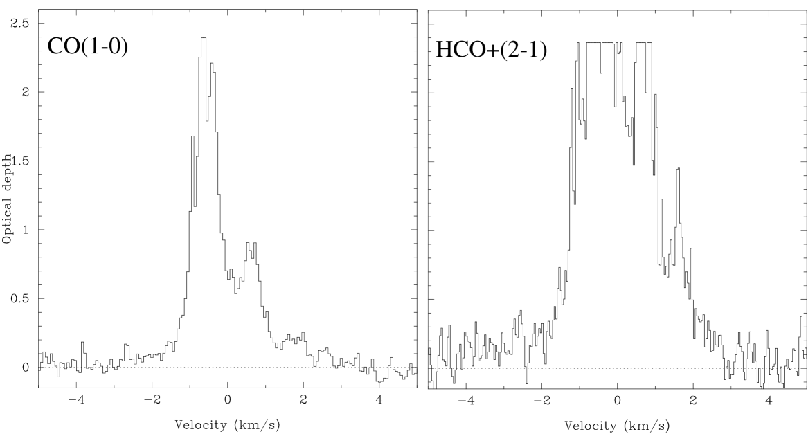
Figure 1: Plots of the observed opacity for the CO(1-0) and HCO⁺(2-1) transitions seen at $z=0.25$ towards PKS1413+135. The cut-off at opacities $>2$ are due to saturation of the signals. The opacity of the HCO⁺(2-1) line is larger than that of the CO(1-0) line despite of an abundance which is $10^{-3}-10^{-4}$ that of CO.

3.3 Known Molecular Absorption Line Systems

There are four known molecular absorption line systems at high redshift: z$=$0.25-0.89. These are listed in Table 2 together with data for the low redshift absorption system seen toward the radio core of Centaurus A. For the high redshift systems, a total of 18 different molecules have been detected, in 32 different transitions. This includes several isotopic species: C¹³O, C¹⁸O, H¹³CO, H¹³CN and HC¹⁸O⁺. As can be seen from Table 2, the inferred H₂ column densities varies by $\sim 10^{3}$. The isotopic species are only detectable towards the systems with the highest column densities: B0218+357 and PKS1830-211, which are also the systems where the absorption originates in lensing galaxies. The large dispersion in column densities is reflected in the large spread in optical extinction, $A_{\rm V}$, as well as the atomic to molecular ratio. Systems with high extinction have 10-100 times higher molecular gas fraction than those of low extinction.

Absorption in the host galaxy.

Two of the four known molecular absorption line systems are situated within the host galaxy to the ‘background’ continuum source: PKS1413+135 wiklind94 and B3 1504+377 wiklind96b . The latter exhibits two absorption line systems with similar redshifts, z$=$0.67150 and 0.67335. The separation in restframe velocity is 330 km s^-1. This is the type of signature one would expect from absorption occurring in a galaxy acting as a gravitational lens, where the line of sight to the images penetrate the lensing galaxy on opposite sides of the galactic center. However, in this case, as well as for PKS1413+135, high angular resolution VLBI images show no image multiplicity, despite impact parameters less than 0$\,.\!\!^{\prime\prime}$1 (e.g. perlman96 xu95 ). The continuum source must therefore be situated within or very near the obscuring galaxy.

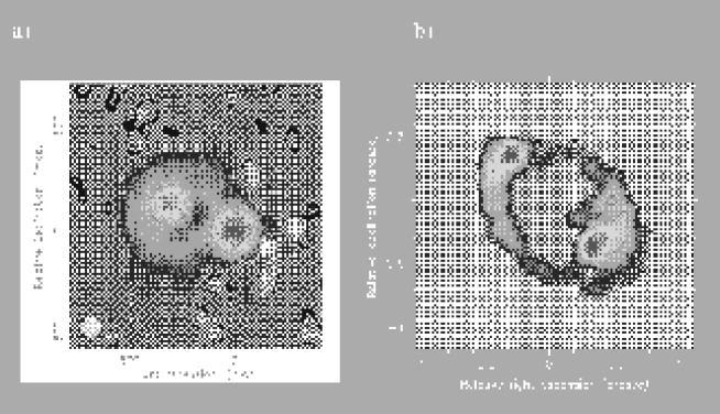
Figure 2: a) A 15 GHz radio image of the gravitational lens B0218+357 obtained with the VLA (courtesy A. Patnaik). b) A 15 GHz radio image of the gravitational lens PKS1830-211.

Figure 3: Channel maps of HCO⁺(2-1) and CO(3-2) absorption towards the B0218+357 obtained with the IRAM Plateau de Bure interferometer. The angular resolution does not resolve the two lensed images of the background QSO. The continuum weakens in the channel maps which corresponds to the absorption line, but never disappears completely. Since the absorption lines are strongly saturated, this shows that only part of the continuum is obscured by optically thick molecular gas. From Combes & Wiklind (unpublished).

Absorption in gravitational lenses.

The two absorption line systems with the highest column densities occur in galaxies which are truly intervening and each acts as a gravitational lens to the background source: B0218+357 and PKS1830-211. In these two systems several isotopic species are detected as well as the main isotopic molecules, showing that the main lines are saturated and optically thick combes95 combes96 wiklind96a wiklind97 . Nevertheless, the absorption lines do not reach the zero level. This can be explained by the continuum source being only partially covered by obscuring molecular gas, but that the obscured regions are covered by optically thick gas. The lensed images of B0218+357 and PKS1830-211 consist of two main components. By comparing the depths of the saturated lines with fluxes of the individual lensed components, as derived from long radio wavelength interferometer observations, the obscuration is found to cover only one of two main lensed components wiklind95a wiklind96a . This has subsequently been verified through mm-wave interferometer data menten96 wiklind97 swift01 .

B0218+357

This is a flat-spectrum radio source lensed by an intervening galaxy. The lens nature was first identified by Patnaik et al. patnaik93 . The lens system consists of two components (A and B), separated by 335 milliarcseconds (Fig 2a). There is also a faint steep-spectrum radio ring, approximately centered on the B component. Absorption of neutral hydrogen has been detected at $z_{\rm d}=0.685$ carilli93 , showing that the lensing galaxy is gas rich. The redshift of the background radio source is tentatively determined from absorption lines of Mg II$\lambda$2798 and H$\gamma$, giving $z_{\rm s}\approx 0.94$ browne93 . Molecular absorption lines were detected in this system wiklind95a further strengthening the suspicion that the lens is gas-rich and likely to be a spiral galaxy. The molecular absorption lines do not reach zero level. Nevertheless, absorption of isotopic species show that the main isotopic transitions must be heavily saturated. In fact, both the ¹³CO and C¹⁸O transitions were found to be saturated as well, while the C¹⁷O transition remained undetected combes95 combes97 . This gives a lower limit to the CO column density which transforms to $N_{H_{2}}\approx 4\times 10^{23}$ cm^-2 and an $A_{\rm V}\approx 850$ mag.

That the molecular gas seen towards B0218+357 covers only one of the two lensed images of the background source can be seen in Fig. 3, where the continuum decreases at velocities corresponding to the absorption line but never completely disappears. Subsequent millimeter interferometry observations have shown that the absorption occurs in front of the A-component, which is then expected to be completely invisible at optical wavelengths. Nevertheless, images obtained with the HST WFPC2 in broad V- and I-band, show both components (Fig. 4). While the intensity ratio A/B of the two lensed images is 3.6 at radio wavelengths patnaik95 , A/B$\approx$0.12 at optical wavelengths. The V$-$I values show no significant difference in reddening for the A- and B-component. Hence, there is no indication of excess extinction in front of the A-component despite the large $A_{\rm V}$ inferred from the molecular absorption. Since it is unlikely that the A/B intensity ratio is very much different at optical and radio wavelengths (differential magnification could introduce a small difference if the radio and optical emission comes from separate regions) the A component appears sub-luminous in the optical. The other possibility is that the B component is over-luminous at optical wavelengths by a factor 30 (or 1.4 magnitudes), possibly caused by microlensing. This latter explanation is, however, quite unlikely in view of the presence of large amounts of obscuring molecular gas in front of the A component. By compiling a sample of flat-spectrum radio sources from the literature, with properties similar to that of B0218+357 (except the gravitational lensing aspect), correcting for different redshift and normalizing the observed luminosities at $\nu=10$ GHz, it is possible to show that the optical luminosity of B0218+357 is abnormally weak wiklind99 (Fig. 4). In this comparison the observed magnitude of the A component was used, multiplied by a factor 1.3 in order to compensate for the B component using the magnification ratio of 3.6. This clearly showed the A component to be sub-luminous, rather than the B component being over-luminous. The interpretation of this is that the A component is obscured by molecular gas, with an extinction that is very large. Some light ‘leaks’ out but through a line of sight which contains very little obscuring gas, hence not showing much reddening in the V$-$I colors. Assuming that all the obscuration occurs in the A component, only $\sim$3% of the photons expected from the A component reaches the observer. Since the extent of the optical emission region is very small, this suggests the presence of very small scale structure with a large density contrast in the molecular ISM of the lensing galaxy.

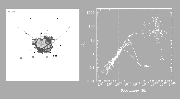
Figure 4: The gravitational lens B0218+357. Left :  Optical image obtained with the HST in the I band (FW814), showing the A and B components (archival data). In contrast to the radio image (Fig. 2a), the A component is weaker than the B component. This is caused by obscuration of molecular gas, which gives rise to the observed molecular absorption lines at $z_{\rm d}=0.688$. Right :  Normalized SED for flat-spectrum radio QSOs. The fluxes for the A component in B0218+357 as observed with the HST are marked by circles. Their positions suggest that only 3% of the flux supposed to come from this component reaches the observer. (From wiklind99 ).

PKS1830-211

This is a radio source consisting of a flat-spectrum radio core and a steep-spectrum jet. It is gravitationally lensed by a galaxy at $z_{\rm d}=0.886$ wiklind96a into two images of the core-jet morphology (Fig. 2b). The two cores are separated by 0$\,.\!\!^{\prime\prime}$97 and the images of the jet form an elliptical ring. PKS1830-211 is situated close to the Galactic center and suffers considerable local extinction. Its lens nature was first suspected through radio interferometry rao88 , but as neither redshift was known nor optical identification achieved (cf. djorgovski92 ) its status as a gravitational lens remained unconfirmed.

The lensing galaxy was found through the detection of several molecular absorption lines at $z_{\rm d}=0.886$ wiklind96a . At millimeter wavelengths the flux from the steep-spectrum jets is completely negligible and it is only the cores that contributes to the continuum. It was soon found that the molecular absorption was seen only towards one of the cores, the SW image. However, weak molecular absorption was subsequently found also towards the NE image. This fortunate situation gives two sight lines through the lens and gives velocity information which can be used in the lens modeling (see Sect. 6). A second absorption line system has been found towards PKS1830-211, seen as 21cm HI absorption at $z=0.19$ lovell96 , making this a possible compound lens system. This intervening system complicates the lens models of this system. A potential candidate for the $z=0.19$ absorption has been found in HST NICMOS images lehar00 . It is situated $\sim$4^′′ SW of PKS1830-211 and is designated as G2. The molecular absorption lines towards PKS1830-211 and their use for deriving the differential time delay between the two cores will be described in more detail in Sect 5.3 and Sect. 6.

4 DUST CONTINUUM EMISSION

The spectral shape of the far-infrared background suggests that approximately half of the energy ever emitted by stars and AGNs has been absorbed by dust grains and then re-radiated at longer wavelengths puget96 fixsen98 lagache99 gispert00 . The dust is heated to temperatures of 20-50 K and radiates as a modified black-body at far-infrared wavelengths. At the Rayleigh-Jeans part of the dust SED the observed continuum flux increases with redshift. This is known as a ‘negative K-correction’ and is effective until the peak of the dust SED is shifted beyond the observed wavelength range, which occurs at $z>10$. Dust continuum emission from high redshift objects is therfore observable at millimeter and submillimeter wavelengths and is an important sources of information about galaxy formation and evolution in general and for gravitational lenses in particular.

4.1 Dust emission

Dust grains come in two basic varieties, carbon based and silicon based. Their size distribution ranges from tens of microns down to tens of Ångströms. The latter are known as PAH’s (Polycyclic Aromatic Hydrocarbonates). Except for the smallest grains, the dust is in approximate thermodynamical equilibrium with the ambient interstellar radiation field. The dust grains absorb the photon energy mainly in the UV and re-radiate this energy at infrared and far-infrared (FIR) wavelengths. The equivalent temperature of the dust grains amount to 15-100 K and they emit as an approximate blackbody.

The spectral energy distribution (SED) of dust emission is usually represented by a modified blackbody curve, $F_{\nu}\propto\nu^{\beta}B_{\nu}(T_{\rm d})$ (cf. thronson86 wiklind95b ), where $B_{\nu}$ is the blackbody emission, $T_{\rm d}$ the dust temperature and $\nu^{\beta}$ is the frequency dependence of the grain emissivity, which is in the range $\beta=1-2$. Such representations have successfully been used for cold dust components where a large part of the SED is optically thin. When $\tau\approx 1$ or larger, the observed dust emission needs to be described by the expression:

$$F_{\nu} = \Omega_{s}B_{\nu}(T_{\rm d})\left(1-e^{-\tau_{\nu}}\right)\ ,$$ (4)

where $\Omega_{s}$ is the solid angle of the source emissivity distribution, $\tau_{\nu}$ is the opacity of the dust. Setting $\tau_{\nu}=\left(\nu/\nu_{0}\right)^{\beta}$ gives $F_{\nu}\propto\nu^{\beta}B_{\nu}(T_{\rm d})$ for $\tau_{\nu}\ll 1$ and $F_{\nu}\propto B_{\nu}(T_{\rm d})$ for $\tau_{\nu}\gg 1$. The critical frequency $\nu_{0}$ is the frequency where $\tau_{\nu}=1$.

The infrared luminosity.

The total infrared luminosity is derived by integrating Eq. 4 over all frequencies. Here the flux density $F_{\nu}$ corresponds to the energy emitted by dust only. The infrared luminosity for an object at a redshift $z$ is given by

$$L_{\rm IR} = 4\pi\left(1+z\right)^{3}D_{\rm A}^{2}\int\limits^{\infty}_{0}{F_{\nu}d\nu}\ ,$$ (5)

where $D_{\rm A}$ is the angular size distance. The solid angle $\Omega$ appearing in Eq. 4 is a parameter derived in the fitting procedure. In the event of a single dust component, $\Omega$ can be estimated from the measured flux $F_{\nu_{\rm r}}$ at a given restframe frequency $\nu_{r}$

$$\Omega = {{F_{\nu_{r}}}\over{B_{\nu_{r}}(T_{\rm d})\left(1-e^{-\left(\nu_{r}/\nu_{0}\right)^{\beta}}\right)}}$$ (7)

$$\approx 6.782\times 10^{-4}\left[{{\nu_{r}}\over{{\rm GHz}}}\right]^{-3}\left[{{{\rm F_{\nu_{r}}}}\over{{\rm Jy}}}\right]\left[{{e^{h\nu_{r}/kT_{\rm d}}-1}\over{1-e^{-\left(\nu_{r}/\nu_{0}\right)^{\beta}}}}\right]\ .$$ (8)

Using some typical values ($T_{\rm d}=30$ K, $\beta=1.5$, $\nu_{0}=6$ THz ($50\mu$m), $\nu_{\rm r}=\nu_{\rm obs}(1+z)=1400$ GHz ($\nu_{\rm obs}=350$ GHz at $z=3$) and, finally, an observed flux of 1 mJy) we get $\Omega\approx 2\times 10^{-14}$. For a spherical source with a radius $r\approx D_{\rm A}\sqrt{\Omega/\pi}$, this corresponds to a dust continuum emission region with an extent of only $\sim 160$ pc.

Although this is a very rough estimate of the size of the emitting region, it shows, since typical observed values were used, that FIR dust emission from distant objects tend to come from very small regions. This will be of importance when considering the effects of gravitational lensing.

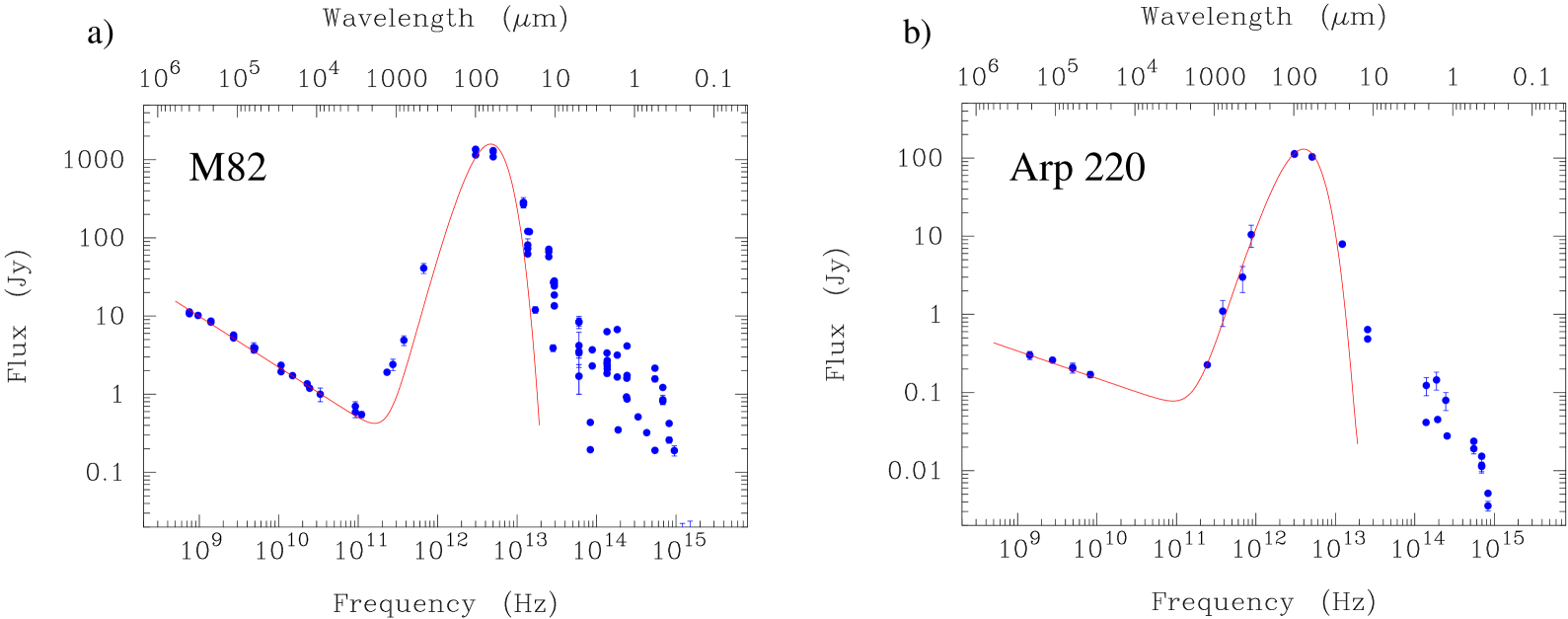
Figure 5: The spectral energy distribution of two starburst galaxies. a) M82 and b) Arp220. Despite a difference in far-infrared luminosity of almost 2 orders of magnitude, their spectral energy distribution are nearly identical. Notice also the presence of cold dust in M82, visible as an excess flux at millimeter and submillimeter wavelengths. The SEDs have been fitted by a modified blackbody curve, which becomes optically thick at 50$\mu$m and which has $\beta=2.0$ for M82 and $\beta=1.3$ for Arp220 and using a single temperature component of T${}_{\rm d}=45$ K for both galaxies.

The dust mass.

An estimate of the dust mass from the infrared flux requires either optically thin emission combined with a knowledge of the grain properties, or optically thick emission and a knowledge of the geometry of the emission region (cf. hildebrand83 ).

The grain properties are characterized through the macroscopic mass absorption coefficient, $\kappa_{\nu}$. Several attempts to estimate the absolute value of $\kappa_{\nu}$ as well as its frequency dependence have given different values (cf. hughes97 ). Combining the same frequency dependence as in hughes97 with a value given by hildebrand83 , the mass absorption coefficient can be described as

$$\kappa_{\nu_{r}} \approx 0.15 \left({{\nu_{r}}\over{375{\rm GHz}}}\right)^{1.5}\ {\rm m^{2}\ kg^{-1}}\ ,$$ (9)

where $\nu_{\rm r}$ corresponds to the restframe frequency. This expression corresponds to a grain composition similar to that found in the Milky Way. At frequencies where the emission is optically thin, the dust mass can now be determined from,

$$M_{\rm d} = {{F_{\nu_{obs}}}\over{\kappa_{\nu_{r}}B_{\nu_{r}}(T_{\rm d})}}D_{\rm A}^{2}(1+z)^{3}\ .$$ (11)

4.2 Detectability of dust emission

A typical far-infrared spectral energy distribution (SED) of a starburst galaxy (M82) is shown in Fig. 5a. The SED of a more powerful starburst (Arp220) is shown in Fig. 5b. Perhaps the most striking aspect of these SEDs is their similarity, despite that they represent galaxies with widely different bolometric luminosities. In both cases most of the bolometric luminosities comes out in the far-infrared: M82 has a far-infrared luminosity of $3\times 10^{10}$ L_⊙, while Arp220 is a so called Ultra-Luminous Infrared Galaxy (ULIRG) with a far-infrared luminosity of $1\times 10^{12}$ L_⊙. The SEDs shown in Fig. 5 have been fitted by a modified blackbody curve, which becomes optically thick at 50$\mu$m and which has $\beta=2.0$ for M82 and $\beta=1.3$ for Arp220 (cf. Eq. 4). The modified blackbody curves has been fitted using a single temperature component of T${}_{\rm d}=45$ K for both galaxies. Notice, however, the presence of a colder dust component in the SED of M82, which is visible as an excess flux at millimeter and submillimeter wavelengths thuma00 .

The observed dust continuum emission originates from dust grains in different environments and which are heated by different sources. Nevertheless, a remarkably large number of dust SEDs, like the ones shown in Fig. 5, can be well fitted by only one, or in some cases two dust components (cf. the cold dust component in M82).

For a single dust temperature component, the flux ratio between the submillimeter (850$\mu$m) and the far-infrared (100$\mu$m) is strongly dependent on the dust temperature. For T${}_{\rm d}=45$ K (as in the case of M82 and Arp220), $f_{850\mu{\rm m}}/f_{100\mu{\rm m}}\approx 3\times 10^{-3}$, while for T${}_{\rm d}=20$ K, $f_{850\mu{\rm m}}/f_{100\mu{\rm m}}\approx 0.06$, or 20 times larger. Nevertheless, as long as the dust temperature is not extremely low, it is much harder to observe the long wavelength tail of the dust SED than the peak at $\sim$100$\mu$m (except that in the latter case one needs to observe from a satellite due to our absorbing atmosphere).

At millimeter and submillimeter wavelengths the SED can, to a first approximation, be characterized by $f_{\nu}\propto\nu^{\gamma}$, where $\gamma=3-4$. Hence, the observed flux increases as an object is shifted to higher redshift. This effect is large enough to completely counteract the effect of distance dimming. An example of this is shown in Fig. 6, where the observed flux at 850$\mu$m has been calculated for a FIR luminous, $5\times 10^{12}$ L_⊙, galaxy, for two different dust temperatures, T${}_{\rm d}=30$ K and T${}_{\rm d}=60$ K, and for two different cosmologies. The largest uncertainty in the predicted flux as a function of redshift comes from the assumed dust temperature, rather than the assumed cosmology. However, regardless of dust temperature and cosmology, the effect of the ‘negative K-correction’ of the dust SED is to make the observed flux more or less constant between redshifts of $z=1$ and all the way to $z\approx 10$, where the Wiener part of the modified blackbody curve is shifted into the submillimeter window and the flux drops dramatically.

This constant flux over almost a decade of redshift range makes the millimeter and submillimeter window extremely valuable for studies of the formation and evolution of the galaxy population at high redshift in general and for gravitational lensing in particular. For a constant co-moving volume density, the submm is strongly biased towards detection of the highest redshift objects. The prerequisite is, of course, that galaxies containing dust exist at these large distances and that the low flux levels expected can be reached by our instruments. Both of these criteria are actually fulfilled; powerful new bolometer arrays working at millimeter (MAMBO, and recently SIMBA) and in the submillimeter (SCUBA) have shown that low flux levels can be observed and that objects containing large amounts of dust do exist at early epochs (cf. hughes98 smail98b eales99 ).

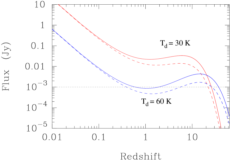
Figure 6: The observed flux density at 850$\mu$m of a source with $L_{\rm FIR}=5\times 10^{12}$ L_⊙ as a function of redshift. The top set of curves correspond to a dust temperature of 30 K and the bottom curves to a dust temperature of 60 K. The full drawn lines correspond to a flat matter dominated universe ($\Omega_{\rm m}=1.0,\Omega_{\Lambda}=0$), and the dashed curve to a flat $\Lambda$ dominated universe ($\Omega_{\rm m}=0.3,\Omega_{\Lambda}=0.7$).

4.3 Submillimeter source counts

One of the first studies using long wavelength radio continuum emission was to simply count the cumulative number of detected sources as a function of flux level. These observations mainly probed high luminosity radio galaxies and showed a significant departure from an Euclidean non-evolving population. This was the first evidence of cosmic evolution ryle67 jauncey75 .

The negative K-correction in the mm-to-far-infrared wavelength regime for dust emission has enabled present day submm/mm telescopes, equipped with state-of-the-art bolometer arrays, to get a first estimate of the source counts of FIR luminous sources at high redshift. There are two bolometer arrays which have produced interesting results so far; SCUBA on the JCMT in Hawaii and MAMBO on the IRAM 30m telescope in Spain. Additional arrays are under commissioning and will likely contribute to this area shortly: SIMBA on the 15m SEST on La Silla, and BOLOCAM on the 10m CSO on Mauna Kea.

The SCUBA bolometer array at the JCMT was put to an ingenious use when it looked at blank areas of the sky chosen to be towards rich galaxy clusters at intermediate redshift smail97 smail98b barger99 blain99b blain99c . The gravitational magnification by the cluster enabled very low flux levels to be reached and several detections were reported. This method has been used by others as well and an example of an image of the rich cluster Abell 2125 at 1250$\mu$m is shown in Fig. 7 carilli00b . More than a dozen sources are detected above the noise but none is associated with the cluster itself. Instead they are all background sources gravitationally magnified by the cluster potential.

The cumulative source count of a population of galaxies is simply the surface density of galaxies brighter than a given flux density limit. In a blank field observation it is in principle derived by dividing the number of sources with the surveyed area. The effects of clustering has to be considered if the observed area is small. In practice there are several statistical properties that have to be considered. Usually the threshold for source detection is not uniform across the mapped area. Since the sources are generally found close to the detector limit those which have fluxes boosted by spurious noise has a higher likelihood to be detected than those which experience a negative noise addition, which are likely to be lost from the statistics. This latter effect leads to an overestimate of the true source flux. The possibility of an additional bias through differential magnification will be discussed in Sect. 4.5.

The case of submm/mm detected galaxies behind foreground galaxy clusters is yet more complicated (cf. blain99b ). The gravitational lens distorts the background area and magnifies the source fluxes. The magnitude of these effects may vary across the observed field. A detailed mass model of the lens is needed in order to transform the observed number counts into real ones, as well as knowledge about the redshift distribution of the sources. Smail and collaborators (smail97 smail98a smail98b ) initially observed 7 clusters, constructed or used existing mass models of the cluster potentials, and managed to obtain source counts at sub-mJy levels (cf. blain99b ). Although the lensing effect of clusters allows observations of weaker fluxes, it introduces an extra uncertainty in the number counts. This is, however, not dominating the overall error budget blain99b . There is another beneficial effect with the lensing in that the extension of the background area alleviates the problem of source confusion. The angular resolution of existing bolometer arrays is approximately 15^′′ and source confusion is believed to be a problem at flux levels below 0.5 mJy.

Other blank field surveys using SCUBA have pushed as deep as the cluster surveys, but without the extra magnification they probe somewhat higher flux levels. Examples of such deep blank field surveys include the Hubble Deep Field North hughes98 , the fields used for the Canada-France Redshift Survey eales99 eales00 , the Lockman hole and the Hawaii deep field region SSA13 barger98 .

All these submm deep fields, including the cluster fields, are only a few square arcminutes. Using on-the-fly mapping techniques a few groups have recently started mapping larger areas but to a shallower depth (cf. borys01 scott01 ).

Carilli et al. carilli00b combined the number counts from all the blank-field observations. The result is a cumulative source count stretching from $\sim$15 mJy to 0.25 mJy (Fig. 8). The source counts obtained using the lensing technique, after correcting for the lensing effects, are compatible with those obtained through pure blank-fields. The turnover at a flux level of $\sim$10 mJy is probably real and represents a maximum luminosity of $\sim 10^{13}$ L_⊙ for an object at $z\approx 3$. The exact shape of the number counts is still uncertain at both the low and high flux ends. Results from the MAMBO bolometer array, which operates at 1250$\mu$m, have been multiplied by a factor 2.25 in order to transform it into the expected flux at 850$\mu$m. This assumes that the objects have an SED of the same type as starburst galaxies (cf. Fig. 5).

In order to transform the cumulative source count into a volume density it is necessary to know the redshift distribution of the sources. It is, however, possible to circumvent this by fitting a model of galaxy evolution to the observed source counts. This has been explored extensively by Blain et al. blain99c , (see also combes99a takeuchi01 ), and will not be discussed further here.

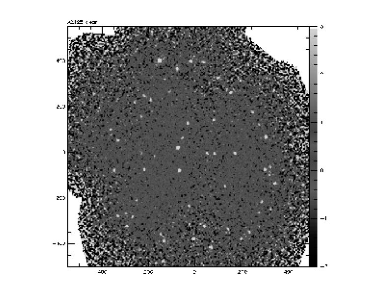
Figure 7: An image of the cluster Abell 2125 obtained with the MAMBO bolometer array at the IRAM 30m telescope (from carilli00b ). The angular size is in arcseconds. The noise rms is at 0.5 mJy/beam.

Figure 8: Source counts from several surveys using SCUBA at 850$\mu$m and MAMBO at 1250$\mu$m (from carilli00b ). The dashed curve is a powerlaw of index $-1.8$ while the solid curve is an integrated Schechter luminosity function with a powerlaw index $-2$ and an exponential cut-off at 10mJy. All fluxes refer to 850$\mu$. The 1250$\mu$m data points have been multiplied by a factor 2.25 in order to transform them into expected fluxes at 850$\mu$m.

4.4 Submm source identification and redshift distribution

The sources detected in submm/mm surveys can in a majority of cases be identified with sub-mJy radio sources (cf. smail00 ). This population of weak radio continuum sources is believed to be powered by star formation rather than AGN activity windhorst85 haarsma00 . Attempts to identify the submm/mm sources with optical and/or infrared counterparts have failed in all but a small number of cases (cf. downes99a ivison00 frayer00 ). The submm/mm detected population is not related to nearby nor intermediate redshift sources, but are believed to be at $z>1$, but the lack of clear optical/IR identifications has made it difficult to assess its true redshift distribution. An alternative technique for determining the redshift has been introduced by Carilli & Yun carilli00a , which relates the radio continuum flux at 1.4 GHz with the measured flux at 850$\mu$m (see also barger00 ). As the radio flux declines with increasing redshift, the submm flux increases (cf. Fig. 5). Although the method is model dependent (mainly depending on the dust temperature T_dust, the radio spectral index as well as the frequency dependence of the dust emissivity coefficient, cf. Sect. 4.1), it gives a rough estimate of the redshift. Using this method it has been possible to show that the majority of the submm/mm detected sources lie at a redshift $1\leq z\leq 4$ (cf. smail00 carilli00b ).

4.5 Differential magnification

One well-known property of gravitational lensing is that it is achromatic, meaning that the deflection of photons by a gravitational potential is independent of wavelength. The achromaticity is applicable to observed gravitational lenses as long as the source size is small compared to the caustic structure of the lens, such as when the Broad Line Region (BLR) of a QSO is lensed by a galaxy sized lens. Chromatic effects can, however, become important if the source is substantially extended (relative to the caustic structure) and the spectral energy density of the source is position dependent.

The submm/mm detected dusty sources discussed in Sect. 4 are characterized by extended emission, several orders of magnitude larger than the compact sources generally studied in gravitational lensing. This applies to dust emission regardless whether the dust is heated by star formation or by a central AGN. Measured on galactic scales, however, the dust is relatively centrally concentrated, with typical scales ranging from $10^{2}$ pc to a few kpc (cf. Sect. 4.1). A dust distribution heated by a central AGN will have a radial dust temperature distribution, even when radiation transfer effects and a disk- or torus-like geometry are considered. This is observed in nearby Seyfert galaxies polletta99 . A radial temperature profile is also found in the case of a pure starburst siebenmorgen99 , but spatially more extended than in the AGN case. Gravitational lensing of an extended dust distribution with a non-homogeneous temperature, and thus emissivity distribution, means that the assumption of achromaticity is no longer valid and the source may be differentially magnified.

If the characteristic length scale in the source plane is $\eta_{0}$ the characteristic length scale in the lens plane is $\xi_{0}=({\rm D}_{\rm d}/{\rm D}_{\rm s})\,\eta_{0}$. Taking a dust distribution of 1 kpc ($\eta_{0}$), a source redshift $z_{\rm s}=3$ and a lens redshift $z_{\rm d}=1$, the characteristic length scale in the lens plane becomes approximately 0$\,.\!\!^{\prime\prime}$2. This is close to the typical image separation for strong lensing. Since the submm/mm detected galaxies are believed to show a significant change in the dust temperature over this scale, it is quite likely that they will exhibit chromatic effects.

An analytical model of the effect of differential magnification of dusty sources was presented in blain99a , where it was shown that the effect can be strong and that it was most likely to produce an increase in the mid-infrared flux relative to the long wavelength flux. This would make the sources appear warmer than what their intrinsic SED would imply.

A more detailed analysis of the effect of differential magnification and its probability for occurance was done by Pontoppidan pontoppidan00 . Using elliptical potentials and a realistic parameterization of the dust and its spectral energy distribution it was showed that both positive and negative distortions of the SED can occur. Here positive means an increase in the mid-IR part and negative means an increase in the far-IR/submm part. Fig. 9 shows a plot of the magnification in a cut through one of these models (elliptical potential) which does not hit the inner tangential caustic. By placing the center of a dust emission region, with a radial temperature profile, well outside the radial caustic (i.e. $>|0\hbox{$\,.\!\!^{\prime\prime}$}5|$ from the center), parts of the outer region of the dust distribution will fall on the high magnification plateau inside the radial caustic and be multiply imaged while the center is singly imaged and only moderately magnified. This situation would cause an enhancement of the long wavelength part of the SED relative to the mid-IR part. The radius of a typical dust distribution is $\sim 0\hbox{$\,.\!\!^{\prime\prime}$}2$ at $z\approx 3$. If the center of the source is placed closer to the radial caustic, both the center and the extended dust distribution will be magnified, but the warmer central dust will experience a larger average magnification and hence result in a flattening of the SED at mid-IR wavelengths. Again, it might be that the cool dust is multiply imaged while the center (possibly containing an AGN) is singly imaged.

Pontoppidan pontoppidan00 found that the cross section for an enhancement of the long wavelength part of the SED is larger than for an enhancement of the mid-IR. However, the latter situation results in a stronger magnification and effects the observed SED to a higher degree. The latter case also represents a situation where the system is more likely to be recognized as a gravitational lens.

Figure 9: Magnification in a cut through the caustic structure of an elliptical lens configuration. The two peaks corresponds to the radial caustic. This particular cut does not pass through the tangential caustic, which would have produced a yet stronger magnification peak close to the center. The length scale is in arcseconds. Notice the very strong gradient in the magnification when going from the one-image region to the the extended three-image ‘plateau’. The magnification changes by a factor $\sim 10$ over angular scales of $\sim 0\hbox{$\,.\!\!^{\prime\prime}$}01$, corresponding to scales of $\sim 50$ pc at $z_{\rm s}\approx 2$. From K. Pontoppidan’s Master Thesis, Copenhagen University pontoppidan00 .

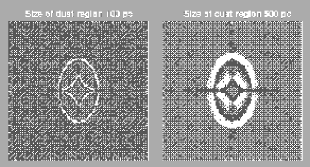
Figure 10: The caustic structure of an elliptical potential showing areas where the dust spectral energy distribution will be influenced by differential magnification. The dust emission region is modeled as a circular disk with a radial temperature profile. The central heating can be either an AGN or a dense starburst. If the center of the dust emission region is placed in the black area, the observed SED will appear cooler than the intrinsic one, while the opposite effect occurs if the center is located in the black areas. The effect of a small (left) and large (right) dust region is illustrated. From K. Pontoppidan’s Master Thesis, Copenhagen University pontoppidan00 .

Effect on number counts of submm/mm detected galaxies.

A distortion map of the effect of differential magnification is shown in Fig. 10 (from pontoppidan00 ). The caustic structure of an elliptical potential representing a central mass surface density of $3\times 10^{9}$ M_⊙ kpc^-2, where the distortion of the dust SED due to differential magnification has been color coded. Black represents a negative distortion (cooler SED) and white represents a positive distortion (warmer SED). The dust distribution of the source is assumed to have a radius of 100 pc (left image) and 500 pc (right image). Quite naturally, the larger the region over which dust is distributed, the larger is the region where negative distortion can occur. By placing the center of the source in the black/white regions of the distortion map, the observed SED will appear cooler/warmer.

The implications for the submm/mm detected objects at high redshift is that differential magnification could induce a bias in the number counts. Especially since in most of the surveys done so far the sources are found close to the detection limit. The effect could induce an overestimate of the number of sources but it could also influence the slope of the cumulative number counts. The latter is more likely but better statistics from surveys reaching low noise levels are needed, as well as a better understanding of the total cross section for positive/negative distortions of dusty submm/mm sources.

An interesting consequence of the differential magnification of these sources is that some, perhaps several, of the detected submm/mm objects may be multiply imaged systems when viewed at high angular resolution in submm/mm wavelengths. The radio identifications that have been done typically reach a resolution of 1^′′ which is not sufficient to see multiple images on the expected 0$\,.\!\!^{\prime\prime}$1-0$\,.\!\!^{\prime\prime}$2 scale. High angular resolution deep imaging with future instruments such as ALMA will resolve this issue.

5 CASE STUDIES

In order to describe in more detail the characteristics of millimeter observations and interpretations of gravitationally lensed sources, as well as to illustrate their use, three cases are presented below. First is the luminous Broad-Absorption-Line (BAL) quasar APM08279+5255 at $z=3.9$. The gravitational lens hypothesis for this source was put forward based only on its apparent luminosity. The second case is a detailed study of the quadruply lensed Cloverleaf quasar, where the gravitational lensing of molecular gas has enabled a more detailed and constrained lens model. The last example is PKS1830-211, where the lensing galaxy was actually first detected through millimetric molecular absorption lines at $z_{\rm d}=0.886$. The molecular absorption lines in this system has been used to constrain the lens model by giving the velocity dispersion and are used to derive the differential time delay between the two main lensed components.

5.1 APM08279+5255: A case of differential magnification?

This object was discovered serendipitously during a search for Galactic carbon stars irwin98 . It was found to be a BAL QSO at a redshift $z=3.911$ (see downes99b for the redshift determination). With an astounding R-band magnitude of 15.2 and detection in three of the four IRAS bands, its bolometric luminosity turns out to be $5\times 10^{15}$ L_⊙. This in itself led to the suspicion that it is a gravitationally lensed object Subsequent observations, both from the ground and from space ledoux98 egami00 ibata99 , led to the detection of three components, with a maximum separation of $0\hbox{$\,.\!\!^{\prime\prime}$}35\pm 0\hbox{$\,.\!\!^{\prime\prime}$}02$, and with a flux ratio of the two brightest components of $1.21\pm 0.25$ (cf. Fig. 13). The optical spectra of the two main components are similar to each other ledoux98 . No lensing galaxy has been identified, although the weak third image could potentially be the lens (see below). Nevertheless, based on the small separation of the main components, their similar spectra and the enormous luminosity inferred for the system, the lensing nature of this system is not questioned. Even in the case of strong gravitational magnification, APM08279+5255 is an intrinsically very luminous system, with L${}_{\rm bol}\geq 10^{13}$ L_⊙.

The high apparent brightness of APM08279+5255 has allowed a very good S/N optical spectra of the intervening absorption line systems to be obtained with the HIRES spectrograph on Keck ellison99 . Several potential lens candidates are found as MgII absorption line systems, with the most conspicuous one at $z=1.181$. Placing the third image at this redshift, however, requires the lens to be unusually compact and luminous. It would need to be almost 5 magnitudes brighter than an L^⋆ galaxy with the relevant velocity dispersion of $\sim 150$ km s^-1 ibata99 egami00 . The possibility that the lens harbors an AGN can be dismissed since no emission lines from $z<3.9$ are detected in the spectrum. Also, the continuum of an intervening QSO should have been detected in the saturated parts of the absorption lines seen towards the background source. No such emission is detected (cf. ellison99 ). APM08279+5255 could thus represent a ‘text book’ example of a gravitational lens with an odd number of components.

Apart from being luminous at optical and UV wavelengths, APM08279+5255 also contains large amounts of dust and metal rich molecular gas (Fig. 11). The SED of APM08279+5255 is actually dominated by a strong dust continuum emission (Fig. 12), detected over a wide wavelength band: from the restframe submm to mid-infrared bands. This puts APM08279+5255 in the class of hyperluminous IR galaxies even when correcting for a strong gravitational magnification.

The overall dust spectral energy distribution is characterized by a steeply rising long wavelength part, with a change of slope around $\lambda_{\rm rest}=200\mu$m, and a flat mid-IR part. The dust continuum spectra can be fitted by two dust components. One ‘cool’ characterized by a dust temperature of T${}_{\rm d}=200$ K, which is optically thin at $\lambda>200\mu$m (cf. Fig. 12). The second component is hot, with T${}_{\rm d}\approx 910$ K, close to the sublimation temperature of carbon based dust grains. This second component is optically thick. The total dust mass, uncorrected for gravitational magnification, is $2\times 10^{8}$ M_⊙, most of it contained in the cool dust component.

The CO emission lines shown in Fig. 11 includes the high excitation transition $J=9-8$. The CO $J=9$ level is $J(J+1)\times 2.77=249$ K above the ground state. Normal type Galactic molecular clouds with typical H₂ densities of $\sim 300-10^{3}$ cm^-3 are not sufficient to collisionally populate the CO $J=9$ level. The mere detection of the CO(9-8) line therefore shows that the gas has to be unusually dense and warm. This immediately suggests that this gas component resides close to the QSO, possibly associated with the hot dust component. If both the CO $J=4-3$ and $J=9-8$ emission are associated with the same gas component, the total molecular gas mass, corrected for magnification, is quite modest: $3\times 10^{9}$ M_⊙ downes99b . If the lower transition, on the other hand, emanates from a more extended and cooler region than the $J=9-8$ transition, the total molecular gas mass can be one to two orders of magnitude larger. That this is likely to be the case was shown by the detection of CO $J=1-0$ and $J=2-1$ emission from APM08279+5255 (Papadopolous et al. 2001). Using the same conversion factor between H₂ column density and velocity integrated CO intensity as is used for the Milky Way and nearby galaxies, the total molecular gas mass in APM08279+5255, uncorrected for gravitational magnification, is $(0.6-3.2)\times 10^{11}$ M_⊙ papadopoulos01 . The amount of gravitational magnification is in this case expected to be low due to the extended nature of the molecular gas, especially the gas seen in the lower transitions. Incidentally, three additional CO emitting sources are detected within 3^′′ of the center of APM08279+5255 papadopoulos01 . If these are not gravitationally lensed images, which they are not if the currently best lens models are used (cf. ibata99 egami00 ), these three additional sources are not magnified to any significant degree. The field around APM08279+5255 should then represent a remarkable over-density of gas rich galaxies at high redshift. These three additional sources are, however, not detected in continuum emission with the Plateau de Bure interferometer nor at optical or NIR wavelengths and their exact nature remains undetermined.

APM08279+5255 has a SED which is essentially flat from a restframe wavelength of $\sim$30$\mu$m to optical wavelengths (cf. Fig.12). This is usually interpreted as being the effect of a face-on configuration of a dust-disk surrounding a central AGN. The low inclination of the disk enables the observer to get an un-obscured view of the hot dust close to the AGN as well as the cool dust further away. Comparison with dust models calculated by Granato et al. granato96 granato97 shows that the mid-IR slope is too shallow even for the most extreme face-on models lewis98 , i.e. the dust SED in APM08279+5255 appears to be too ‘warm’ even if heated by a powerful AGN. Another possible explanation for the flat mid-IR SED is that APM08279+5255 experiences differential magnification of the dust emission region. This possibility was explored by Egami et al. egami00 by applying sources of various sizes to their lens model. In Fig. 12 the SED of APM08279+5255 is shown together with a starburst model rowanrobinson93 . The starburst model has been arbitrarily fitted to the long wavelength part of the observed SED. At mid-IR wavelengths, the starburst model predicts a flux which is $\sim$50 times lower than the observed fluxes in APM08279+5255. The data points marked by open circles are the equivalent observed fluxes diminished by a factor of 50 in order to fit the starburst model. Although APM08279+5255 undeniably contains a powerful AGN, which is likely to contribute a substantial part of the heating of the gas and dust, the influence of star formation can not be ruled out. Can differential magnification account for at least part of the difference between a pure starburst SED and the observed one?

Figure 11: CO spectra and maps of APM08279+5255 observed with the IRAM Plateau de Bure interferometer (Downes et al. downes99b ). Upper left: 1.4mm dust continuum. Lower left: CO(9-8) emission. Upper and lower right: CO(4-3) and CO(9-8) emission line profiles. The angular resolution of the maps is $3\hbox{$\,.\!\!^{\prime\prime}$}2\times 2\hbox{$\,.\!\!^{\prime\prime}$}3$, far too coarse to resolve the individual components seen at optical/NIR wavelengths. The maps are centered on $08^{\rm h}31^{\rm m}41\hbox{$\,.\!\!^{\rm s}$}70,\ +52^{\circ}45^{\prime}17\hbox{$\,.\!\!^{\prime\prime}$}35$ (J2000).

Figure 12: The spectral energy distribution of APM08279+5255 fitted by two isothermal greybody models. The full-drawn line corresponds to the sum of a ‘cool’ component (T${}_{\rm dust}=200$ K) and a hot component (T${}_{\rm dust}=910$ K). The dust emission becomes optically thick at $\lambda<200\mu$m. The data points (filled circles) are from Irwin et al. irwin98 , Ledoux et al. ledoux98 , Lewis et al. lewis98 , Downes et al. downes99b , Egami et al. egami00 and the Faint Source IRAS catalog (NED). The dotted line is a starburst model of Rowan-Robinson & Efstathiou rowanrobinson93 , which has been arbitrarily fitted to the long wavelength part of the SED. The data points marked by open circles are the equivalent observed data points but with their values reduced by a factor 50 in order to fit on the starburst model.

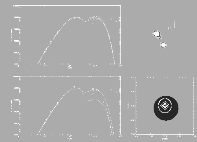
Figure 13: The 2-image and 3-image lens model solutions for APM0927+5255 and their effect on the spectral energy distribution. In the 2-image solution (top left), the intrinsic mid-IR part of the SED is slightly depressed, while in the 3-image solution (bottom left) the intrinsic mid-IR is strongly enhanced (representing a positive distortion, see Sect. 4.5). The intrinsic SED is represented by dashed and dotted lines, for a dust distribution with a radius of 600 pc and 300 pc, respectively. The full drawn line is the observed SED. In the top right is APM08279+5255 seen with the HST WFPC2 camera and lower right is the dust model and its location used in the 3-image solution. From K. Pontoppidan’s Master Thesis, Copenhagen University pontoppidan00 .

Modeling the lens APM08279+5255.

The lensing configuration of this system has been modeled by Egami et al. egami00 and Ibata et al. ibata99 . Using an isothermal elliptical potential with no external shear, two different types of lens models were applied: a three-image model and a two-image model. The former model is non-singular in order to produce the third image, while the latter assumes that the third image is the lensing galaxy and the potential is singular in order to suppress the formation of the third image. The two-image model produce a modest magnification of $\sim$7 (cf. egami00 ), while the three-image model produce a magnification of $\sim$90 for both a point source and a more extended source distribution ibata99 egami00 . Since the apparent bolometric luminosity exceeds $10^{15}$ L_⊙, the three-image configuration is more appealing. However, the core radius is large, 0$\,.\!\!^{\prime\prime}$21, almost as large as the Einstein radius, 0$\,.\!\!^{\prime\prime}$29. If the lens is at a redshift $z_{\rm d}\approx 1.2$, the core radius corresponds to $\sim$1.2 kpc in the lens. This is much larger than most measured core radii. In a survey of 42 giant elliptical galaxies it was found that the objects which can be resolved have a median core radius of 225$h^{-1}$ pc lauer85 . In the case of a three-image model, the potential is almost circular with $\epsilon=0.012$, while the two-image model gives $\epsilon=0.083$ egami00 . The difference in ellipticity corresponds to a difference in the size of the caustic structure, which in turn influences the effects of differential magnification. In the three-image model, the caustic structure is approximately 45 pc in extent in the source plane, while the two-image model has a caustic structure almost 5 times larger.

The effects on the lensing behavior for a source with a finite extent was explored in egami00 . A source with an extent exceeding $\sim 500$ pc resulted in a filled disk. A more detailed model was done by Pontoppidan pontoppidan00 where an assumed source temperature distribution was used in order to derive the resulting spectral energy distribution. Using the model parameters of egami00 , where the source is located between the radial and tangential caustic for the three-image model, the hot dust is expected to be moderately enhanced by the outer magnification plateau (cf. Fig. 10). In the two-image scenario, the QSO is again located outside the tangential caustic. In this case, however, the radial caustic is lacking due to the singular potential. The latter scenario can produce a modest negative distortion of the SED (as seen in the top left panel of Fig. 13). In the three-image scenario, however, the effect on the SED is more dramatic and represents a positive distortion, i.e. the mid-IR part of the SED is enhanced relative to the long wavelength part (bottom left panel of Fig. 13). The magnitude of the distortion is quite large, its details depending on the extent of the dust region. For a dust distribution with a radius of 650 pc, the differential magnification can enhance the intrinsic flux at restframe mid-IR wavelength with a factor $\sim 10$. A smaller extent of the dust results in a smaller enhancement factor. The dust region (for a radius of 300 pc) and the caustic structure are seen in the lower right panel of Fig. 13.

The three-image model of APM08279+5255 is more likely to be correct than the two-image model since it produces a magnification which corresponds to a source with a bolometric luminosity which is large, but not extreme. The three-image model also means that for realistic dust distribution, the restframe mid-IR is strongly enhanced relative to the longer wavelength part of the SED. The intrinsic SED of APM08279+5255 resembles that of less extreme dusty QSO spectra (cf. carilli00b ). In fact, the shape of the intrinsic SED of APM08279+5255 now resembles that of pure starburst models, except that the mid-IR is still enhanced by a factor $5-10$, marking the influence of the AGN. This shows that the effects of differential magnification must be considered before applying radiation transfer models to gravitationally lensed dusty sources.

In order to model the resolved and extended low-J CO emission, the effects of a highly elliptical lensing potential has been explored lewis02 . The lensing galaxy is here assumed to be an edge-on spiral. The result is a good fit with the extended low-excitation CO emission, while the point sources from the background QSO, although imaged into three components, have widely different magnification ratios compared to the observed values. This may not be of great importance if microlensing affects the optical photometric results (e.g. lewis99 ).

5.2 The Cloverleaf: Another case of differential magnification

The Cloverleaf is the gravitationally lensed image of the BAL quasar H1413+117 at $z=2.558$, showing four quasar-images (hereafter called spots) with angular separation from 0$\,.\!\!^{\prime\prime}$77 to 1$\,.\!\!^{\prime\prime}$36. Since its discovery magain88 , the Cloverleaf has been imaged with ground based telescopes in numerous bands up to I and with HST/WFPC2 in the UV, optical and near-IR turnshek97 kneib98a kneib98b .

The lensing system.

After the early lens model of Kayser et al. kayser90 , these new data sets have been used to derive an improved model of the lensing system kneib98a kneib98b which now includes:

1. A cluster of galaxies with derived photometric redshifts in the range 0.8 to 1.0, which contributes to the magnification.

2. A lensing galaxy close to the line of sight to the quasar, which determines the geometry of the image (four main spots) and carries the largest share of the magnification. The redshift of the lensing galaxy has been tentatively measured with VLT/ISAAC at a value of 0.9 (Faure et al. in prep).

In the following, we use this new model for the lensing system, which is essentially constrained by the HST data. Further details can be found in kneib98a kneib98b .

The IRAM millimeter data sets.

After its discovery in the CO(3-2) line emission with the IRAM Pico Veleta dish barvainis94 , the Cloverleaf has been observed in the millimeter range by various teams and instruments (wilner95 with BIMA, yun97 with OVRO). Yet, the best data sets collected to date on this object are from the IRAM Pico Veleta dish and Plateau de Bure interferometer.

A total of six millimeter transitions have been reported from observations with the IRAM Pico Veleta dish: CO(3-2), CO(4-3), CO(5-4), CO(7-6), CI(³P₁-³P₀) and HCN(4-3) barvainis97 . Detailed non-LTE modeling of the CO line strengths by these authors indicates that the molecular gas is warm (T larger than 100 K), dense ( n(H₂) density larger than $3\times 10^{3}$ cm^-3) and not very optically thick ($\tau_{\rm CO}<3$). These results suggest that the molecular material is close to a powerful heating source and might therefore be related to the environment of the central engine in the quasar. They also prompt us for not using the conventional conversion factor CO to H₂ which is derived for molecular clouds in the disk of our Galaxy.

Thanks to the strength of the CO(7-6) transition, a high resolution (0$\,.\!\!^{\prime\prime}$5) map was obtained with the IRAM Plateau de Bure interferometer. A first CO(7-6) interferometric data set alloin97 has later been complemented with observations at intermediate baselines kneib98a . The combined data has lead to the CLEANed map restored with an 0$\,.\!\!^{\prime\prime}$5 circular beam, shown in Fig. 14 . In order to search for a velocity gradient, we have derived the spatially integrated line profile, following the procedure described in alloin97 . The CO(7-6) line profile (Fig. 15) shows a marked asymmetry with a steep rise and excess of emission (with respect to a standard Gaussian) on its blue side and a slower decrease on its red side. Excluding the central velocity channel (so that the split in velocity is symmetric), we have built the blue (-225, -25 km/s) and the red (+25, +225 km/s) maps displayed in Fig. 14c,d respectively. The difference between the red and blue CLEANed maps (Fig. 14b) establishes firmly the presence of a velocity gradient at the 8$\sigma$ level. Measurements of the characteristics of the spots from the CO(7-6) image have been performed (spot flux ratios, sizes and orientations) through a fitting procedure in the visibility domain, as explained in alloin97 . Final parameters are provided in Table 1 of kneib98a where the spot sizes are intrinsic to the image, i.e. deconvolved by the interferometer beam: spots A, B and C definitely appear elongated.

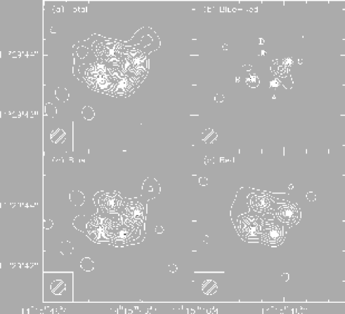
Figure 14: Image of the Cloverleaf obtained with the IRAM Plateau de Bure interferometer kneib98a . a) is the total CLEANed image. c) and d) are the blue and red part of the total emission profile, while b) shows the difference between the CLEANed blue and red images. A velocity gradient in the underlying source can be inferred from the residual. The data has been restored with a circular beam of angular resolution 0$\,.\!\!^{\prime\prime}$5.

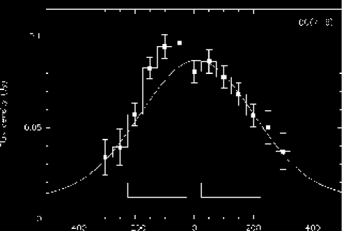
Figure 15: The ¹²CO(7-6) spectrum from the $z=2.56$ Cloverleaf quasar obtained with the IRAM Plateau de Bure interferometer kneib98a . The thin line represents a best fit Gaussian profile. Notice the asymmetric line profile with excess emission at the blue part of the spectrum.

Comparing images in the UV and the millimeter range.

Images in the UV/optical correspond in the quasar restframe to the emission from the accretion disk surrounding the quasar central engine. This latter source is expected to be point-like. The four spots on the HST images do indeed have a stellar-like appearance, being circular with a FWHM of about 0$\,.\!\!^{\prime\prime}$068 kneib98a . The absolute photometry and relative intensity ratios of the four spots (Table 4 in kneib98a ) have been computed using the Sextractor software bertin96 . The large variation of the intensity ratios in U, compared to V, R and I bands can probably be explained by absorption along the line of sight by intervening galaxies. Alternatively, this effect can be ascribed to dust extinction at the redshift of the quasar, using an SMC-like dust extinction law turnshek97 . The presence of such an absorbing medium in the close environment of the central engine could be put in relation with the BAL appearance of this quasar.

The millimeter CO lines are expected to arise from an extended structure, the so-called dusty/molecular torus, with an intrinsic radius of a few 10 pc to a few 100 pc (according to models). In such a configuration, different parts of the extended torus will be positioned differently with respect to the caustic (the curve which represents in the source plane the signature of the lensing system). As the image properties and the amplification factor in particular, are ruled by the relative positioning of the source/caustic, the four spots on the CO(7-6) image, each corresponding to the extended torus, will be distorted with respect to the four spots on the HST image (corresponding each to a point-like source). This features what is called ‘differential magnification effects’ (see Sect. 4.5). From the blue bump appearing on the CO(7-6) line profile (Fig. 15), we clearly see that the blue-shifted part of the CO line arises from a region of the molecular torus which is positioned closer to the caustic than the region emitting the red-shifted side of the CO line. In this way, we are able to recover detailed structural and kinematical information about the molecular torus in the quasar.

In order to derive precisely the shear induced by the lensing system on the extended source in the quasar, it is imperative to register with a high accuracy the Cloverleaf image in a waveband corresponding to a point-like source in the quasar (accretion disk: UV restframe, that is an R band image for example) and in a waveband corresponding to an extended source in the quasar (molecular torus: CO(7-6) line). The high precision required, better than 0$\,.\!\!^{\prime\prime}$2, was achieved using a combination of the HST data and of CFHT data acquired over a larger field of view under extremely image quality kneib98a .

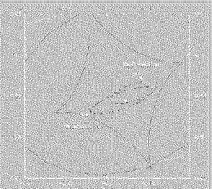
Figure 16: The caustic structure and the CO source distribution in the Cloverleaf quasar kneib98a . The central ellipses represent the CO source distribution for the red and blue part of the emission profile, respectively. The dot in the center corresponds to the quasar UV point source. The scale on the axis is arcseconds. The result has been obtained by combining an HST optical image with the interferometric CO data.

Derived properties of the molecular torus in the Cloverleaf BAL quasar at $z=2.558$.

We have used the model of the lensing system as constrained by the HST data and presented above. The total amplification factor for the CO emission is found to be 30. This amplification factor translate to a molecular gas mass M(H${}_{2})=2\times 10^{9}$ M_⊙ and an atomic hydrogen gas mass M(HI)$=2\times 10^{9}$ M_⊙ barvainis97 kneib98a .

We have derived the properties of the molecular torus in the quasar using the CO(7-6) maps: firstly using the total line flux and secondly, using separately each of the blue and red halves of the CO(7-6) line kneib98a . We find a typical size for the molecular torus of 150 pc (assuming H${}_{0}=50$ km s^-1, $\Omega_{m}=1$ and $\Omega_{\Lambda}=0$). When we treat separately the maps corresponding to the blue-half line and red-half line, we find that the quasar point-like UV source is almost exactly centered between the region emitting the blue-half of the CO line and the region emitting the red-half of the line (Fig. 16). This is reminiscent of a disk- or ring-like structure orbiting the quasar at about 75 pc and with a Keplerian velocity of 100 km s^-1 (assuming a disk orientation perpendicular to the plane of the sky). The resulting central dynamical mass would be about $8\times 10^{8}$ M_⊙. This value is in good agreement with the estimate of the molecular gas mass made above from the total CO line flux, provided uncertainties in the inclination of the molecular torus and in the conversion factor from I(CO) to N(H₂).

In conclusion, we can regard the case of the Cloverleaf as a first and enlightening example of what will become routine when ALMA becomes available. Indeed, exploiting differential magnification effects is an extremely promising technique. The effective angular resolution on the CO source in the quasar at $z=2.558$, using this procedure, is $\sim$0$\,.\!\!^{\prime\prime}$03, or about 17 times smaller than the synthesized beam of the IRAM observations! And the amplification factor in this case is around 30!

5.3 PKS1830-211: Time delay and the Hubble constant

Observations and applications of differential time delays in gravitational lenses are discussed in detail elsewhere in this book. Here some results which have implications for the millimetric part of the electromagnetic spectrum will be presented. More specifically, we will discuss a derivation of the differential time delay in the gravitational lens PKS1830-211 obtained from the saturated molecular absorption line of HCO⁺(2-1).

The gravitational lens system PKS1830-211 has been described in some detail above (Sect. 3.3). The background quasar is variable at radio wavelengths, with an amplitude which increases at shorter wavelengths. This is due to the fact that the core, where the variability occurs, is a flat-spectrum source while the jet, which has a more or less constant flux, has a steep radio spectrum. It is presently unknown if PKS1830-211 is variable at infrared/optical wavelengths, although this is likely to be the case.

Time delay measurements of the PKS1830-211 system has also been done using long wavelength radio continuum ommen95 lovell98 . In one case a single dish telescope was used and the two main lens components were not resolved ommen95 . The analysis had to be based on a compound light curve and the derived time delay of $44\pm 9$ days should therefore be regarded as tentative. In the other case, the ATCA interferometer was used, with an angular resolution that did not fully resolve the NE and SW components lovell98 . Instead a model fitting procedure was used in order to obtain two separate light curves over an 18 months period. The resulting differential time delay is $26^{+4}_{-5}$ days. Although the analysis is model dependent, this result represents a considerable improvement in the $\Delta t$ estimate.

Time delay measurements using molecular absorption lines.

As discussed in Sect. 3.3, the lens in the PKS1830-211 system was first detected through molecular absorption lines at a redshift $z_{\rm d}=0.88582$ wiklind96a . More than 16 different molecular species in 29 different transitions have so far been detected at millimeter wavelengths wiklind96a wiklind98 gerin97 . Two additional molecular species in three different transitions have been observed at cm wavelengths menten99 .

The millimeter transitions include three different isotopic variants: H¹³CO⁺, HC¹⁸O⁺ and H¹³CN. The mere detection of these lines shows that the main isotopic transitions of these molecules must be highly saturated. Despite this the absorption lines do not reach zero intensity (Fig. 17b). This can only be reconciled with an optical thick obscuration that do not completely cover the background continuum emission. In fact, from the ratio of the total continuum and the depth of saturated molecular absorption lines (such as HCO⁺(2-1), HCN(2-1), etc.), it was concluded that only the SW lens component is obscured by molecular gas and that the covering factor of this particular image is unity or close to unity wiklind96a . A secondary weaker molecular absorption has now been found towards the NE component as well, separated in velocity by $-147$ km s^-1 wiklind98 .

Imaging of the HCO⁺(2-1) absorption line with the IRAM millimeter wave interferometer did not directly resolve the NE and SW components wiklind98 . This is due to the low declination of the source relative to the latitude of the interferometer, creating a synthesized beam elongated in approximately the same direction as the image separation. The continuum, however, is strong enough to allow self-calibration, making it possible to accurately track the phase center. The best angular resolution is achieved in right ascension ($\sim 0\hbox{$\,.\!\!^{\prime\prime}$}1$) with a factor $\sim$2 worse resolution in declination due to an elongated synthesized beam. At frequencies outside the absorption line, the phase center should fall on a line in between the NE and SW components. Assuming that the flux ratio NE/SW is similar to that derived for longer wavelengths ($\sim 1.3-1.4$), the phase center should move towards positive RA at frequencies where the absorption occurs. If the covering factor is unity, $\Delta\alpha$ should be $\sim+0\hbox{$\,.\!\!^{\prime\prime}$}25$. This is exactly the amount of shift observed for the saturated HCO⁺(2-1) line (Fig. 17a). A similar shift in the declination of the phase center can also be seen and concurs with these results wiklind98 . This result has also been confirmed through BIMA observations where the two continuum components have been separated swift01 .

Due to this fortunate configuration of obscuring molecular gas in the lensing galaxy, the flux contributions from the NE and SW cores can easily be estimated using molecular absorption lines and a single dish telescope with low angular resolution. The 15m SEST telescope, which is used for the time delay monitoring presented here, has a HPBW of $\sim$50^′′ at the observed frequency of the HCO⁺(2-1) transition, much larger than the image separation of 0$\,.\!\!^{\prime\prime}$97. Since molecular gas covers only the SW component, as shown by the interferometric data, and the line opacity is $\gg 1$ as seen from the rare isotopic lines, the depth of the absorption line corresponds to the flux from the SW component only. The total continuum away from the absorption line corresponds to the sum of fluxes from the SW and NE components (Fig. 18).

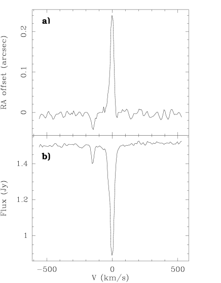
Figure 17: Bottom: Spectrum of HCO⁺(2-1) at $z=0.886$ towards PKS1830-211 obtained with the IRAM interferometer. The main absorption line is seen around zero velocity. A secondary, weaker absorption line of HCO⁺(2-1) is seen at a velocity of $-147$ km/s relative to the main line. Top : The right ascension shift of the phase center of the continuum emission as a function of velocity. A negative shift means that the phase center moves towards the NE component, while a positive shift indicates a shift towards the SW component. Comparison with the absorption spectra shows that the main absorption component covers the SW source, while the weaker secondary absorption covers the NE source. (From wiklind98 .

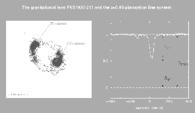
Figure 18: Illustration of how the individual light curves of the NE and SW components can be derived from the single dish millimetric observations. A 5 GHz radio image of PKS1830-211 subrahmanyan90 shows the two cores and the extended jet emission. At millimeter wavelengths only the cores contributes to the continuum emission. The right hand panel shows the saturated HCO⁺(2-1) spectrum. Since the molecular gas only covers the SW component and the line opacity is $\gg 1$, the depth of the absorption line corresponds to the flux from the SW component only. The total continuum away from the absorption line corresponds to the sum of the fluxes from the SW and NE components.

Monitoring of HCO⁺(2-1).

Monitoring of the HCO⁺(2-1) absorption and the total continuum flux has been going on at the 15m SEST telescope since April 1996. Data can only be obtained between February and November due to Sun constraints (PKS1830-211 comes within 3^∘ from the Sun). The light curves are shown in Fig. 19. Since only the total continuum (at the top in the figure) and the depth of the absorption line (at the bottom in the figure) are measured, the flux from the NE component (middle) is derived as the difference $T_{\rm NE}=T_{\rm tot}-T_{\rm abs}$, and therefore has a somewhat higher uncertainty. During the 1996-2000 campaigns a total of 144 usable observations have been obtained. The background quasar had a large outburst during 1998. The outburst shows a single peak in the total continuum, putting an upper limit to the differential time delay between the two cores (no double peak structure). Separating the light curves for the two cores, however, one can clearly see a delayed response of the SW image relative to the NE (Fig. 19). This is seen even more clearly when plotting the ratios of the NE and SW fluxes (Fig. 20). This ratio shows the relative magnification of the two cores and should be constant in the absence of a time delay. The decrease in the flux ratio during the 1998 outburst is a clear indication of the time delay between the NE and SW cores.

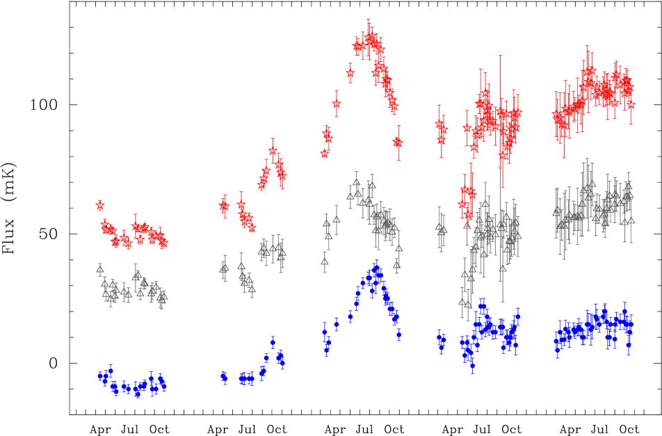
Figure 19: Results from 5 years of monitoring of the HCO⁺(2-1) absorption at $z_{\rm d}=0.886$ towards PKS1830-211. The top curve shows the measured total continuum flux away from the absorption line. Notice the large outburst during 1998. The bottom curve shows the depth of the HCO⁺(2-1) line (shifted by $-30$ mK). This corresponds to the flux from the SW component. The middle curve shows the flux derived for the NE component.

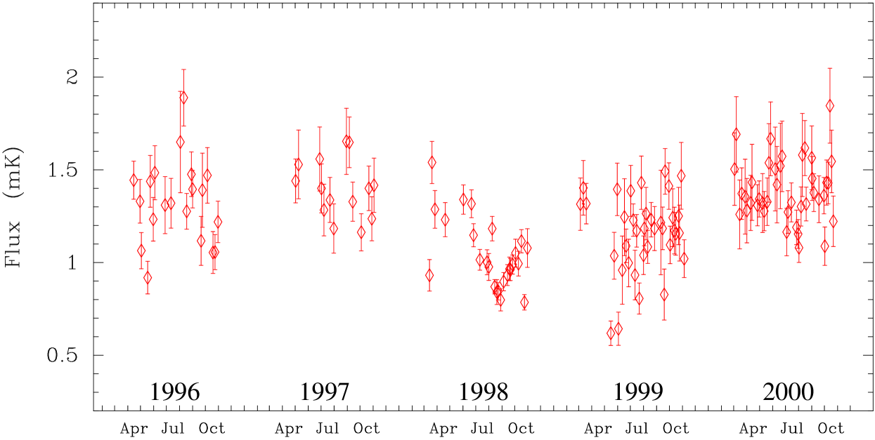
Figure 20: Same as Fig. 19 but showing the flux ratio of the NE and SW components.

Monitoring results.

The light curves shown in Figs. 19 and 20 have been analyzed using several different techniques. The problem is straightforward: correlate two unevenly sampled time series. However, the analysis is complicated by the fact that since the two time series are really copies of each other but shifted in time they are effectively sampled at different epochs.

There are two main types of methods used for obtaining the time delay. One is to interpolate unobserved data points and then apply standard techniques for cross correlation. The other is to use the unevenly sampled time series and try to correlate neighboring points as good as possible. The former method is superior if the sampling rate is high, but this is usually not the case for astronomical data. The latter method has less precision but is the least unbiased way of obtaining the time delay. Both types of methods have been used for the molecular absorption line data on PKS1830-211.

Data analysis.

The observables at each epoch $t_{i}$ are the total continuum flux $S_{0}(t_{i})$ and the depth of the absorption line, corresponding to the flux from the SW component $S_{SW}(t_{i})$. The total continuum is the sum of the two image components,

$$S_{0}(t_{i})=S_{1}(t_{i})+S_{2}(t_{i})\ \ ,$$

where subscript 1 refers to the NE component and 2 to the SW component. We know that the $S_{1}$ and $S_{2}$ fluxes are related as

$$S_{1}(t_{i})=\mu\,S_{2}(t_{i}+\Delta t)\ \ ,$$

where $\mu$ is the magnification ratio and $\Delta t$ the differential time delay between the two cores. Hence,

$$S_{0}(t_{i})=\mu\,S_{2}(t_{i}+\Delta t)+S_{2}(t_{i})\ \ .$$

By shifting the observed $S_{2}$ values, multiplying it with a magnification ratio and adding the observed unshifted and unmagnified values we should recover the observed total flux at time $t_{i}$. Since the observations consist of an unevenly sampled time series, with significant amount of noise, finding the true $\Delta t$ and $\mu$ is a non-trivial exercise.

The analysis of the light curves has been done using three methods. Two of them involves interpolating between the observed data points and construction of an evenly sampled time series. Due to the rather long interruptions due to the Sun avoidance, interpolation only extends over periods between February and November. An elaborate interpolation scheme of unevenly sampled data has been developed with the specific goal of resolving the time delay controversy of 0957+561 (Press et al. press92 ). In the case of the molecular absorption data, however, a smoothing function with an effective resolution similar to the average data point separation at each epoch was applied. Using the smoothed time series, data points in between observed epochs were linearly interpolated. The smoothing dampens the worst fluctuations while retaining the small scale structure in the time series. It also allows an easy assessment of the relative weights of observed and interpolated data. A complication, however, is that the data points are no longer completely independent. This is of some concern when deriving the reduced $\chi^{2}$ values.

$\chi^{2}$ minimization :

Minimization was done using both the time delay $\Delta t$ and the magnification ratio $\mu$ as well as keeping the magnification ratio fixed or time dependent. The latter is due to a surprising realization that the magnification ratio might be variable, albeit on a much longer time scale than the time delay (cf. Fig. 20). Using a parameterized $\mu(t_{i})$ means that the solution becomes cumbersome and slow. Instead we smoothed the flux ratio and fitted a third order polynomial. This parameterization of $\mu(t_{i})$ was used when solving for $\Delta t$. The result, together with results from the other analysis methods, is shown in Fig. 21 and gives a $\Delta t=27$ days.

Cross correlation :

Edelson & Krolik edelson88 developed a discrete cross correlation method specifically aimed for reverberation mapping of AGNs that can be used for time delays in gravitational lensing. The method optimizes the binning of data points rather than the interpolation, as in the method of Press et al. press92 . The method requires a fairly well sampled data set to start with in order to retain a sufficiently good temporal resolution. The sampling rate for molecular absorption line data in PKS1830-211 is not dense enough to use the Edelson & Krolik method. Instead cross correlation was done on the same smoothed and interpolated data set as the $\chi^{2}$ minimization. The cross correlation coefficient is defined as $r_{\rm ab}=s_{\rm ab}^{2}/(s_{\rm a}\,s_{\rm b})$, where the covariances $s_{\rm a}$ and $s_{\rm b}$ are defined in the usual manner (cf. bevington92 ). As with the $\chi^{2}$ minimization, the data points are not entirely independent due to the smoothing and interpolation and the variances are only approximately true. The result gives $\Delta t=25$ days, with a rather broad maximum for the cross correlation coefficient (Fig. 21).

Minimum dispersion (the Pelt method) :

A simple and robust technique for analyzing unevenly sampled time series was presented by Pelt et al. pelt94 pelt96 . They successfully applied it to the lens system 0957+561. The strength of the method is that interpolation or smoothing are not needed, leaving the errors for each data point independent. The method is a form of cross correlation where a given data point is correlated with a data point which is temporally its closest neighbor. The method is illustrated in Fig. 22, where the round and square markers in the two top rows represent the two photometric data sets obtained from a two-component gravitational lens. When correlating the time series, one of them is shifted in time, as the square markers in the middle rows. Projecting both the unshifted (round) and the shifted (square) time series to a common array (bottom row), correlation is done between those data points which are from different time series and closest to each other. These points are connected by arcs in the figure. It is easy to include the effects of different magnifications for the lensed components as well as time delays in systems with two or more lenses pelt98 .

The results are undeniably noisier than for the interpolated data sets. This can be seen in Fig. 23, where the Pelt dispersion method has been applied to both raw and interpolated data. The best fit is for a time delay $\Delta t=28$ days, with the NE component leading.

Error analysis :

The errors associated with the light curves are a combination of noise in the data points and systematic errors. The latter can originate in the instrument, in the modeling necessary for separation of the lensed components (as in the case of long wavelength radio observations), assumptions made about the lensing system, etc. When interpreting the time delay in terms of a Hubble constant, the largest systematic error comes from modeling of the gravitational potential (see Chapter X). Noise in the data comes from imprecise measurements but can also originate in secondary variability such as microlensing and interstellar scintillation. The latter is applicable at long radio wavelengths. Microlensing may be of importance even for gravitational lenses observed at radio wavelengths (cf. koopmans00 ).

In order to assess the significance of correlations found in the light curve of gravitationally lensed images it is customary to derive the confidence limits through Monte Carlo simulations and bootstrap techniques (cf. fassnacht99 ). The results often shows non-Gaussian distributions and confidence levels are set by finding the range of delays and magnification ratios inside which a given amount (say 95%) of the simulations lie. This gives a better estimate of the true confidence level than simply fitting a Gaussian to the distribution. Doing this for the molecular absorption line data in PKS1830-211 gives a time delay of $\Delta t=28^{+4}_{-5}$ days, with the NE component leading.

In Fig. 24 the light curve of the SW component in PKS1830-211 has been shifted by $-28$ days and multiplied by a magnification ratio $\mu$. In the upper panel a constant ratio of $\mu=1.3$ was used, while in the lower panel a time dependent magnification ratio was used. The use of different parameterizations of the magnification ratios do not change the derived time delay, but the time dependent form provides a better fit of the two light curves. The reason for the slow change in magnification ratio is presently unclear. It may have implications for the use of molecular absorption lines as a probe of the time delay, but since the time scale for the change of the magnification appears to be much longer than the time delay, it is likely to be of small importance when correlating light curves for each period (i.e. 9 months).

Figure 21: The time delay for PKS1830-211 derived from molecular absorption lines and using cross-correlation, $\chi^{2}$ minimization and the Pelt Minimum Dispersion method. All three methods in this example use the interpolated data set.

Figure 22: Illustration of the Pelt Minimum Dispersion method used to determine time delays in gravitational lenses. This method was one of the methods used for deriving the time delay in PKS1830-211 from molecular absorption lines. This particular case shows a two-image lens (A and B), where the respective light curves are sampled at irregular intervals. In the middle section the B light curve is shifted by $\Delta t$. By projecting the resulting data points to a common array (C), nearest neighbors of different light curves are correlated (arcs). A weight, depending on the time difference between the points used in the correlation, can be applied.

Figure 23: Results for the time delay of molecular absorption lines in the PKS1830-211 gravitational lens system using the Pelt Minimum Dispersion method. Both raw and interpolated data sets are shown (left and right, respectively). Also shown are the results for different treatments of the magnification ratio. In the top two rows, the magnification ratio is included in the fit, while in the two bottom rows the magnification ratio is predetermined by fitting either a second or third degree polynomial to the observed magnification ratio.

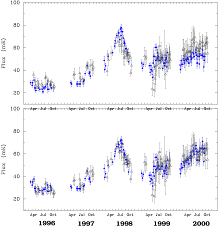
Figure 24: The light curve of the SW component in PKS1830-211 (black) shifted by $\Delta t=-28$ days and multiplied by a magnification ratio $\mu$. The light curve for the NE component is shown in grey. In the upper panel a constant magnification ratio of $\mu=1.3$ was used, while in the lower panel a time dependent magnification ratio was used (cf. Fig. 23).

6 LENS MODELS FOR PKS1830-211

In order to use the differential time delay to derive a value for the Hubble constant, a lens model has to be fitted to the observed data. This is not a trivial exercise in most cases and this is particularly true for PKS1830-211. Due to its location at Galactic longitude $l=12.2^{\circ}$ and latitude $b=-5.7^{\circ}$, PKS1830-211 suffers considerable Galactic extinction. In addition, the molecular gas seen in absorption towards the SW component contributes significant obscuration for at least this image. Early attempts to identify the radio source PKS1830-211 with an optical counterpart were all unsuccessful subrahmanyan90 djorgovski92 . It was only with the advent of sensitive infrared imaging and spectroscopical capabilities that progress could be made. The NE image was positively identified using K-band imaging at Keck and the ESO NTT courbin98 . While the redshift of the lens, $z_{\rm d}=0.886$, had been derived using molecular absorption lines wiklind96a , the redshift of the source was obtained from near-infrared spectroscopy lidman98 . The redshift was found to be $z_{\rm s}=2.507$. Imaging with the HST WFPC2 and NICMOS allowed identification of both the NE and SW image lehar00 . In addition, an object which might be the lensing galaxy was detected (designated as G). Its exact center position remains uncertain due to the presence of a point source $\sim 190$ mas away. The nature of the point source remains unknown but could possibly be a Galactic star and thus of no importance for the lens model. In a recent paper by Courbin et al. courbin02 combined images from the HST and Gemini-North telescopes show what might actually be the lensing galaxy at $z_{\rm d}=0.889$. The lens has two spiral arms, as expected from the molecular absorption data. One spiral arm crosses the SW image of the QSO. The center of the spiral is, however, significantly offset from the line joining the NE and SW images. Based on symmetry arguments, the center of the lensing galaxy is believed to be in the proximity of this line joining the images (Fig 25).

All the necessary ingredients for a detailed lens model are thus in place, except for two remaining uncertainties: the exact position of the lensing galaxy and the possible double-lens nature of the system (cf. Sect. 3.3).

Figure 25: Illustration of the positions of various components in the PKS1830-211 gravitational lens system. The two cores are marked by QSO (NE) and QSO (SW). The putative location of the lens galaxy, derived by Lehár et al. lehar00 , is marked by ‘G’ (filled circle) and a point source of unknown origin is marked by ‘P’ (star). A new possible lens location (from courbin02 ) is marked by ‘S’ (filled triangle). The location of the center of the lens derived from the lens model here, using the Lucy rectification scheme, is marked by ‘Lucy’ (open circle), the lens center derived by Nair et al. nair93 by ‘NRR93’ (open diamond) and the lens center derived by Kochanek & Narayan kochanek92 by ‘KN92’ (open rectangle). The dashed line joining the two QSO images is only to guide the eye.

6.1 Early models

There have been several attempts to model the lens system PKS1830-211. The system was first detected at radio wavelengths, where it is a prominent southern radio source. The morphology of the system was found to be that of a double, while the radio spectrum is typical for a compact flat-spectrum source. This led Rao & Subrahmanyan rao88 to first suggest that PKS1830-211 is a gravitationally lensed system. Based only on the radio images and their polarization properties, obtained with the Very Large Array (VLA) at 5 and 15 GHz, Subrahmanyan et al. subrahmanyan90 constructed a lens model which is not much different from later ones based on more detailed data. In order to reconstruct the extended radio structure, Subrahmanyan et al. modeled the source as an one-sided core-jet structure. To get lensed images with a morphology similar to the observed one, they also had to include a ‘knot’ in the jet. Based on their lens model Subrahmanyan et al. predicted a time delay of $27\,h_{100}^{-1}$ days (using the now known redshift of the source and the lens).

Nair et al. nair93 modeled the PKS1830-211 system using improved radio interferometry data (cf. jauncey91 ). The method was similar to that of Subrahmanyan et al. subrahmanyan90 in that the source structure was built up in a piecemeal manner in order to fit various observed features. With this type of method one can emphasize the influence of small and weak features which may carry a small weight in an inversion scheme based on $\chi^{2}$ minimization of model$-$observed results, but may nevertheless carry important information on the lensing scenario. In the PKS1830-211 system such a weak radio feature, labeled E, was used by Nair et al. to constrain the lens model. This feature might be a third demagnified image of the core. However, since the flux of the E component is less than one percent of the peak value, its significance in terms of flux is small unless the dynamic range of the interferometry maps is very good. Nair et al. found that an elliptical potential with the radio core located close to the inner edge of the radial caustic gave a good fit to the observed morphology. As in the previous model by Subrahmanyan et al. subrahmanyan90 , it was necessary to include a ‘knot’ feature in the source distribution. The jet needed to be bent and cross the tangential caustic. The model gives a good fit to the observed system and places the lens galaxy close to, but not coinciding with, the possible lens position observed by Lehár et al. lehar00 . The estimated time delay, using the known source and lens redshifts, is $17\,h_{100}^{-1}$ days.

A difficulty with extended lensed images is that any inversion must solve simultaneously for both the lens configuration and the source structure. This type of inversion problem can be seen as

$$I_{obs}(\zeta) = \int{\psi(\zeta^{\prime})\,K(\zeta-\zeta^{\prime})}\,d\zeta^{\prime}\ \ ,$$ (12)

where both the source distribution $\psi(\zeta)$ and the kernel $K$ (here representing the lensing potential) are unknown. This type of problem is generally unsolvable. In the case of lensing, however, one can use the knowledge that when the lensed image contains multiple distorted components of the background object these must arise from a common source. Furthermore, it is known that surface brightness is conserved. These ‘priors’ constrain the problem and permit the simultaneous solution of both the structure of the source and the properties of the lensing potential. This type of inversion problems for gravitational lenses has been developed extensively by Kochanek, Wallington and collaborators in several papers (cf. kochanek89 kochanek92 wallington96 ). In particular, Kochanek & Narayan kochanek92 developed an inversion method based on the CLEAN routine (cf. hogbom74 ) used in radio interferometry data reduction and applied it to PKS1830-211. This method takes into consideration the effects of the finite resolution when attempting to invert the lens model and is thereby able to better distinguish the best lens model. The LensClean method of Kochanek & Narayan has produced the hitherto most reliable model for the PKS1830-211 system, but due to the finite resolution, the inversion was done on radio data with rather low angular resolution but with good signal-to-noise, it is not likely to represent the final model.

Lehár et al. lehar00 modeled the PKS1830-211 system using a singular isothermal elliptical mass distribution as well as with two singular isothermal spheres representing the lens galaxy and the source G2 (cf. Sect. 3.3). In both these cases they fixed the lens at the position of G, with a positional uncertainty of 80 mas. The extended radio emission was not used to constrain the lens model. Lehár et al. noted the strong dependence of the location of the lens galaxy and the Hubble constant derived from differential time delay measurements.

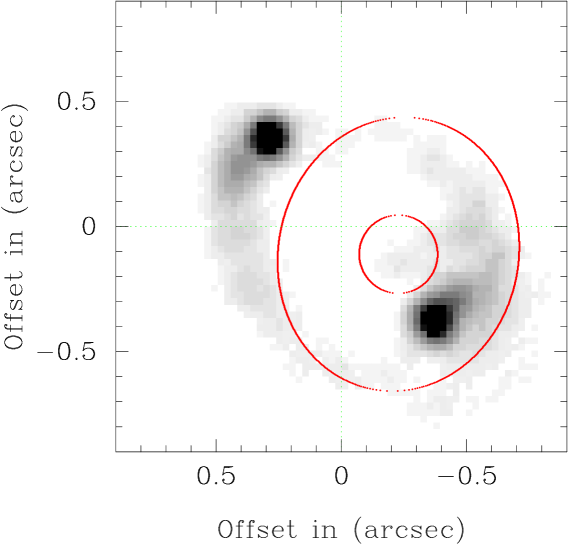
Figure 26: A 15 GHz radio image of PKS1830-211 (from subrahmanyan90 ). The center of the coordinate system is arbitrary. All positions in the text and in Table 3 are relative the NE image. The critical lines of the best fit lens model, shown in Fig. 27 are shown for comparison.

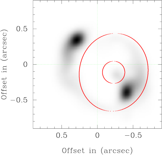
Figure 27: The lensed images obtained from inversion of the lens equation using Lucy rectification and Simulated Annealing (as described in the text). In this particular solution, the lens is fixed at the position of the observed (putative) lens center $G$ (see Fig. 25). The critical lines from the lens model are marked.

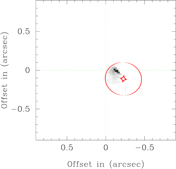
Figure 28: The source distribution derived from the best fit lens model, which gives the image seen in Fig. 27. The caustic structure is shown.

6.2 A new lens model of PKS1830-211

The situation is rather unsatisfactory concerning the various solutions to the lensing configuration characterizing PKS1830-211. Three different models (kochanek92 nair93 lehar00 ) give three different positions for the lens, with corresponding differences in the value of the Hubble constant for a given time delay. The situation is summarized in Fig. 25. The location of the cores in the long wavelength radio data used by Kochanek & Narayan kochanek92 differ from that used by others (using data from shorter wavelengths). Their lens center relative to the other features shown in Fig. 25 is therefore somewhat uncertain.

The fact that surface brightness is conserved can be used in modeling a lensing configuration if both the observations and the code have infinitely good resolution. In the opposite extreme, if the source remains unresolved, one can calculate the magnification for a point source and apply a smoothing function (convolution) representing the observational transfer function (e.g. atmosphere, telescope, imaging array). A more difficult situation arises when an extended source distribution is partially resolved by the observer. A given resolution element will represent different areas of the source in a rather complicated manner and the conservation of surface brightness ceases to be a good prior for an observed lens system. In their LensClean method Kochanek & Narayan kochanek92 solves this situation by representing the source emissivity distribution by $\delta$-functions, mapped through the lens configuration with the corresponding magnification ‘turned on’ and then smoothed by a restoring beam.

An alternative way to solve the inversion problem as stated above is presented here. A more thorough description of the method will be published in Wiklind (2002). The concept is similar to the LensClean method of Kochanek & Narayan kochanek92 . However, instead of introducing CLEAN components, as $\delta$-functions to represent the source distribution, this method starts with a none-zero smooth source distribution and applies the Lucy rectification method lucy74 to constrain the source emissivity, given the observed lensed images and for a given lens model. The Lucy rectification scheme has been used extensively to deconvolve images obtained with the Hubble Space Telescope before the corrective optics was installed. It has also been used to deconvolve the molecular gas distribution in galaxies observed with single dish telescopes of rather poor angular resolution wiklind92 wiklind93 .

The method has an outer loop, which controls the lensing parameters, and an inner loop which solves for the best source distribution given the lens configuration. In the inner loop the source distribution is mapped through the lens and the resulting image is compared with the observed one. The source distribution is adjusted according to the Lucy method (see below) and the process is repeated. When the inner loop has converged, the source distribution is mapped through the lens a final time and the resulting image gives a goodness-of-fit. The lensing configuration is then modified in the outer loop and the process is repeated. The Lucy method is used only in the inner loop, each time starting with a perfectly smooth source distribution. The observed images are represented by

$$I_{obs}(x_{1},x_{2}) = \int{\int{\psi(y_{1},y_{2})\,K(x_{1},x_{2}|y_{1},y_{2})\,dy_{1}dy_{2}}}\ \ ,$$ (13)

where $\psi(y_{1},y_{2})$ is the true source distribution and $K(x_{1},x_{2}|y_{1},y_{2})$ is the kernel representing both the gravitational lens and the finite angular resolution of the observation. The kernel is here written as a conditional probability function: the likelihood of $(x_{1},x_{2})$ given $(y_{1},y_{2})$. With this formulation we can use the Lucy method in a straightforward manner. The idea being that an approximation to the true source distribution is

$$\psi^{n+1}(y_{1},y_{2}) = \psi^{n}(y_{1},y_{2})\,\int{\int{\frac{I_{obs}(x_{1},x_{2})}{I^{n}(x_{1},x_{2})}\,K(x_{1},x_{2}|y_{1},y_{2})\,dx_{1}dx_{2}}}.$$ (14)

The conditional probability function $K$ contains the likelihood of an image emissivity at position $(x_{1},x_{2})$ given a source emissivity at $(y_{1},y_{2})$ and the action of a restoring beam (i.e. a finite angular resolution). The simplest (although not entirely correct) restoring beam is a Gaussian with a HPBW similar to the angular resolution of the observations.

Even starting with a constant source emissivity distribution $\psi^{0}$, the Lucy rectification converges very rapidly to a specific source distribution. Unfortunately, there is no good criteria for determining when to stop the rectification (cf. lucy74 ). In this particular application the inner loop was stopped after 5 iterations of the Lucy rectification. The outer loop consists only of changing the lensing parameters. Several different methods can be employed for this, the most efficient for this application being the Simplex method. However, there is a risk that this method gets stuck in a local minimum and great care has to be taken to ensure that a global minimum has really been reached. This involves repeatedly restarting the Simplex method with parameters offset from the ones giving a (local?) minimum in the $\chi^{2}_{\nu}$. An alternative method that circumvents this, but that is computationally more expensive, is Simulated Annealing (cf. metropolis53 wiklind92 ). This latter method was used in this application.

The lens was modeled as a non-singular elliptical mass distribution

$$\kappa(x_{1},x_{2}) = \kappa_{0}\,\left(x_{1}^{2}+\frac{x_{2}^{2}}{q^{2}}+s^{2}\right)^{-\gamma}\ \ ,$$ (15)

where $q$ is the projected axis ratio, $s$ is the core radius and the surface density profile is set to $\gamma=1/2$, representing an isothermal mass distribution. The deflection angle and magnification was calculated using the code developed by Barkana barkana98 . This code can handle surface density profiles with $\gamma\neq 1/2$, but here the modeling is restricted to the isothermal case. The density profile is, however, a very important parameter when deriving the Hubble constant using differential time delays (cf. williams00 koopmans99 ). In all there are six lens parameters that were fitted: the center position of the lens, the position angle, the velocity dispersion, the ellipticity, and the core radius.

Applying this method to the 15 GHz radio image of PKS1830-211 shown in Fig. 26 subrahmanyan90 , a best fit lens model is achieved with the parameters as tabulated in Table 3. Also listed in Table 3 are the results when keeping the lens position fixed at the coordinates of the putative infrared lens center G. The resulting image distribution for case (b) is seen in Fig. 27 together with the critical lines of the lens. The corresponding source distribution is seen in Fig. 28 together with the caustic structure.

The two solutions presented in Table 3 are very similar to each other, yet they give quite different values to the Hubble constant. Using the lens model of Nair et al. nair93 , the Hubble constant becomes H${}_{0}=59^{+11}_{-8}$ km/s/Mpc. These differences are mainly due to the different locations of the lens center and introduces a large uncertainty in the correct value of H₀.

The lens model presented here will be further refined and the results should be regarded as tentative. However, unless the position of the lens can be derived more accurately, the value of the Hubble constant will remain uncertain. As mentioned above, the shape of the density profile is also a source of uncertainty for a more exact derivation of H₀. This uncertainty is largest for exponents $\gamma<1/2$ koopmans99 .

Table 3: Lens parameters

	6 free parameters		4 free parameters
			(lens fixed)
lens centera	-0.5008	-0.5205	-0.5010	-0.4450b
$\kappa_{0}$	0.3196		0.3106
$q$	0.8576		0.8991
$s$	0.0929		0.0745
PA	135.553		101.174
$\left(\frac{\Delta t}{28^{\rm days}}\right)^{-1}$H${}_{0}^{c}$	$63^{+14}_{-6}$		$83^{+18}_{-9}$

$(a)$ Relative to the NE component.
$(b)$ Fixed at possible lens center G lehar00 .
$(c)$ With $\Delta t=28^{+3}_{-5}$ days.

7 FUTURE PROSPECTS

Existing millimeter and submillimeter telescopes use gravitational lenses more as an aid to the study of distant objects, rather than being an aid to the study of gravitational lensing as such. Nevertheless, some information about the content of the interstellar medium in both lenses and sources have been obtained, and the molecular absorption lines seen towards PKS1830-211 have been used to measure the differential time delay in this particular system.

This situation will change dramatically when planned telescopes at millimeter and submillimeter wavelengths become available. Increased sensitivity and angular resolution will make this wavelength regime very important for studies of gravitational lenses as a phenomenon of their own. The most obvious advantage is that obscuration effects will be completely absent. The effects of microlensing will also be absent or at least minimal. The use of flux ratios of lensed components for constraining parameters when modeling lensed have fallen out of favor due to differential extinction and microlensing effects, but will be usable when the new submm/mm instruments are available.

Existing submillimeter and millimeter facilities include single dish telescopes, such as the IRAM 30m telescope on Pico Veleta in Spain, the JCMT 15m telescope on Mauna Kea, and the SEST 15m telescope on La Silla in Chile. Two 10m size dishes, aimed primarily for submillimeter wavelengths, include the CSO on Mauna Kea and the HHT on Mount Graham in Arizona. These telescopes use both heterodyne receivers for spectral line observations and bolometer type array cameras for continuum observations. The sensitivity depends largely on the quality of the site and the instrumentation. The angular resolution, however, is determined by the diffraction limit of the telescopes. At $\lambda=1$mm, the angular resolution is limited to $10^{\prime\prime}-25^{\prime\prime}$. This constitutes the largest limitation to the study of gravitational lenses. For number counts (see Sect. 4.3) the lack of angular resolution means that with only slightly more sensitive receivers, confusion will become a major limitation (cf. hogg01 )

A few interferometers operating at millimeter wavelengths exist. The IRAM Plateau de Bure interferometer in France consists of five (soon to be six) 15m telescopes, and represents the largest collecting area today. The OVRO interferometer consists of six 10m telescopes, while BIMA consists of eight 6m telescopes. In Japan the Nobeyama interferometer consists of six 10m telescopes. All of these facilities operate at $\lambda=3-1$mm. The angular resolution reached is typically around 1^′′ or slightly better. However, sensitivity becomes a serious limitation at the longest baselines and highest angular resolutions. Also, the Australian Telescope Compact Array (ATCA) has recently been upgraded to work at 3mm with five of its 22m elements.

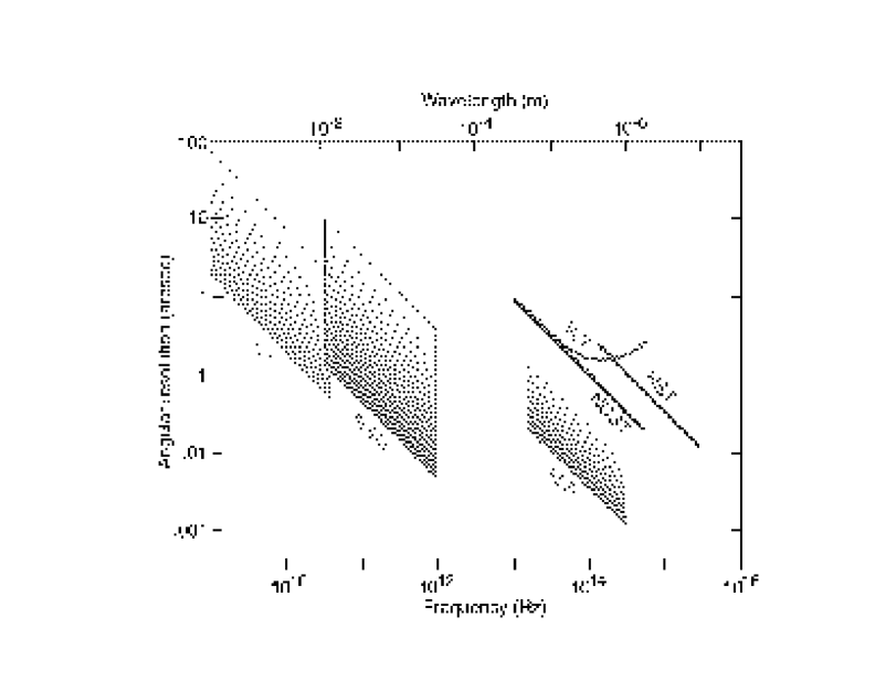
Figure 29: A comparison of the wavelength coverage and the angular resolution of existing and planned instruments. The VLA refers to the Extended VLA. With ALMA, the same angular resolution will be reached from cm wavelengths into the optical.

7.1 Future instruments

Single dish telescopes.

A few single dish submm/mm telescopes are under construction, or in advanced planning. These include the recently commissioned Green Bank Telescope (GBT), which has a 90m unobstructed dish and will reach $\lambda$3mm when fully operational. The Large Millimeter Telescope is a 50m telescope built as a collaboration between INAOE and the University of Massachusetts in Amherst. This telescope will be placed on Sierra Negra in Mexico and operate at a wavelength of 1-4 millimeter. Two single dish telescopes to be situated close to the ALMA site (see below) are under construction: APEX is a 12m, single dish telescope which will be placed on Chajnantor at an altitude of 5000m. This telescope will operate into the THz regime, i.e. $\lambda\sim 300\mu$m. ASTE is a Japanese 10m dish, to be placed at Pampa La Bola, a few kilometers away from the ALMA site. The ASTE will also operate at submm to THz frequencies. These new single dish telescopes will explore distant objects, including gravitational lenses, with somewhat better angular resolution than existing telescopes. Nevertheless, even at the highest frequencies it will only reach an angular resolution of $\sim 6^{\prime\prime}$. This is insufficient for detailed studies of gravitationally lensed systems.

The Atacama Large Millimeter Array.

A major step in submm/mm wave instruments will be the joint European-US project, with Japanese involvement as well, of building a large millimeter and submillimeter interferometer at an altitude of 5000m on Chajnantor in Chile. This instrument, with the acronym ALMA, will consist of $64\times 12$m telescopes, each with a surface accuracy of at least 20$\mu$m. The total collecting area will be 7238 m², which is an order of magnitude greater than the largest existing instrument today. The longest baseline will be $10-12$ km, leading to an angular resolution surpassing that of the Hubble Space Telescope. A rough estimate of the angular resolution power is $0\hbox{$\,.\!\!^{\prime\prime}$}2\,\lambda_{\rm mm}/{\rm L}_{\rm km}$, where $\lambda$ is the wavelength in millimeters and $L$ is the baseline length in kilometers. ALMA will easily reach 0$\,.\!\!^{\prime\prime}$1 resolution and, at the highest frequencies and longest baselines, 0$\,.\!\!^{\prime\prime}$01. A comparison of the wavelength coverage and the projected angular resolution for existing and planned telescopes is shown in Fig. 29.

At the same time ALMA will increase the sensitivity over existing instruments by at least two orders of magnitude. The noise rms level reached with an interferometer consisting of $N$ array elements, each of effective area $A_{\rm eff}$ and with an integration time of $t_{\rm int}$ seconds over an effective bandwidth of $B$ Hz, is expressed as

$$\Delta S = \frac{2k}{A_{\rm eff}}\,\frac{T^{\prime}_{\rm sys}\,e^{\tau_{\nu}}}{\sqrt{N(N-1)\,B\,t_{\rm int}}}\ \ ,$$ (16)

where the term $e^{\tau}$ represents the damping by the atmosphere at frequency $\nu$. The system temperature, $T^{\prime}_{\rm sys}$, is the total noise received by the telescope (including ground pick-up). From this expression it is clear that large individual antenna sizes, a large number of array elements, a large bandwidth, a low system temperature and as little damping from the atmosphere are essential for a sensitive interferometer. These criteria can be fulfilled by using state-of-the-art receiver systems and putting them at a high and dry site such as Chajnantor in the Andes.

The excellent atmospheric conditions at Chajnantor is estimated to give a total system temperature (including the atmospheric damping) of $\sim$230 K at a wavelength of 0.8mm. Using a 16 GHz wide backend and one hour of integration, the 5$\sigma$ detection limit will be 100 $\mu$Jy. At a wavelength of 460 $\mu$m the corresponding 5$\sigma$ detection limit after one hour is 1 Jy. Although considerably worse, this wavelength range is usually not reachable at all with ground-based facilities. These values are representative for unresolved sources. If the source is resolved at the longest baselines, the sensitivity decreases.

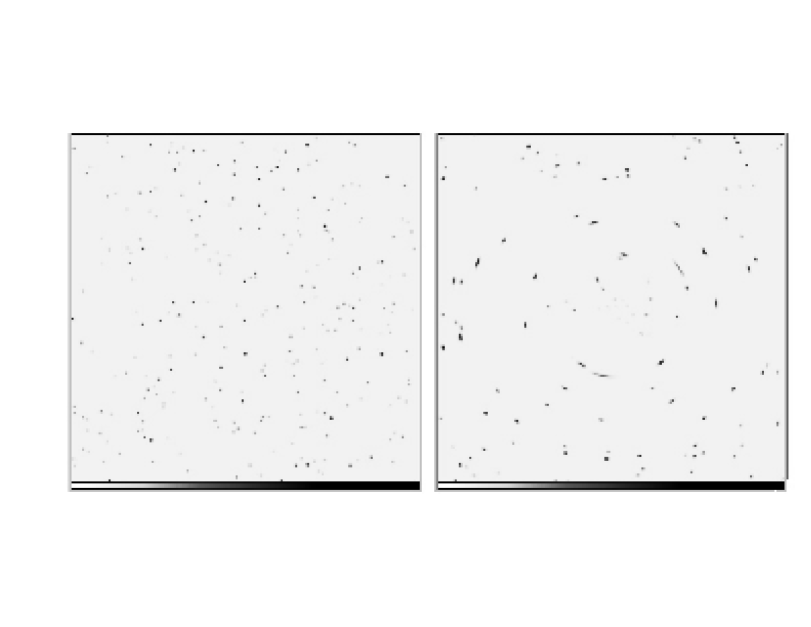
Figure 30: A simulated 9 arcmin² deep field observed with ALMA at a wavelength of 850$\mu$m. All sources above the 5$\sigma$ noise rms limit of 0.15 mJy are shown. The source population was modeled to fit the observed cumulative source counts, extrapolated to 0.1 mJy using a more shallow powerlaw than what can be fitted in the range 1-10 mJy. Left: Unlensed field. Approximately 210 sources are ‘detected’. Right: The same field as in the left image but with an intervening rich galaxy cluster at redshift $z=0.3$.

7.2 Weak lensing at submillimeter wavelengths

With its superb sensitivity and angular resolution, ALMA can successfully be used to study weak lensing by intermediate redshift galaxy clusters. Assuming a constant co-moving volume density of dusty high redshift objects, the constant sensitivity to dust continuum emission from $z\approx 1$ to $z\approx 10$ (Sect. 4.2) favors the detection of the highest redshift objects. This selection bias is unique for the submm/mm wavelength regime. Furthermore, a reasonably well-sampled $uv$-plane, resulting from a large number of interferometer elements, will have a point-spread function (PSF) which is well behaved in comparison to existing wide-field CCDs. And, finally, the dust distribution in galaxies tend to be symmetric and centrally concentrated, leading to a simple geometry of the lensed sources. The latter issue is, of course, not well constrained by existing data. Although dust continuum emission will be easier to detect at large distances than line emission (cf. combes99b ), the high sensitivity and broad instantaneous bandwidth of ALMA will allow CO lines to be observed for many of the lensed sources. This enables a direct way of deriving the redshift distribution of the source population. Furthermore, observations of CO lines in the intervening galaxies will allow a determination of the dynamical mass of the lenses.

ALMA will, however, have a relatively limited instantaneous field of view. This is particularly aggravating at high frequencies. The field of view is limited by the size of the individual telescopes and will be similar in size to that of existing single dish telescopes. This means that the time consuming process of mosaicing is necessary. The key parameters for the effectiveness or speed of this new instrument are the sensitivity $\Delta S$, the angular resolution and the primary beam area $A_{\rm fov}$. The time required to survey a given area $A$ to a flux density limit $S$ is then: $t\approx(\Delta S/S)^{2}(A/A_{\rm fov})$ (cf. blain99d blain96 ).

An example of what can be achieved with ALMA is shown in Fig. 30. The left panel shows a simulated 9 arcmin² field observed with ALMA to a 5$\sigma$ noise rms limit of 0.15 mJy. The wavelength is 0.8mm and was chosen to maximize the number of detected dust continuum sources while minimizing the observing time (by making the field-of-view as large as possible). The field of view per pointing is $\sim$0.07 arcmin². As shown in Sect. 7.1 it takes somewhat less than one hour of telescope time to reach this 5$\sigma$ detection limit. To cover 9 arcmin² thus requires a total of 130 hours. In this example more than 200 sources will be detected (left panel) and their distortion by a rich cluster at $z=0.3$ will be clearly detectable (right panel). In this example a population of dusty galaxies was assumed to have a constant co-moving volume density between $z=1-7$ and undergo pure luminosity evolution. The observed flux densities were fitted to the number counts derived from SCUBA and MAMBO observations (Sect. 4.3). The median luminosity of the ‘detected’ galaxies is $3\times 10^{11}$ L_⊙ and their redshift distribution is more or less flat between $z=2$ to $z=7$. The cumulative source counts was not, however, extrapolated to weaker flux densities using the same powerlaw as applicable between 10-1 mJy (cf. Fig. 8, but with a more modest slope. This ensures that the number of sources seen in the right panel of Fig. 30 is not an overestimate.

In the same manner as lensing by intermediate redshift clusters is presently being used to observe dust continuum sources at flux density levels otherwise not reachable with existing instruments, ALMA will reach flux densities approaching $\mu$Jy levels when observing lensed sources. For high redshift galaxies, this flux density level corresponds to luminosities around $10^{9}$ L_⊙, i.e. dwarf galaxies.

8 SUMMARY

The study of gas and dust at high redshift is important for several reasons. It gives us an unbiased view of star formation activity in obscured objects and it tells the story of the chemical evolution and star formation history in galaxies through the amount of processed gas (and dust) it contains. With today’s millimeter and submillimeter facilities, this research area has used gravitational lensing mostly as a tool to boost the sensitivity. This is evident through the preponderance of gravitationally lensed objects among those which have been detected at $z>2$ in the lines of the CO molecule. It is also evident in the use of lensing magnification by galaxy clusters in order to reach faint submm/mm continuum sources. There are, however, a few cases where millimeter lines have been directly involved in understanding lensing configurations. The best example of this is the highly obscured PKS1830-211, where the lens was identified through molecular absorption lines and where these lines give a velocity dispersion measure by originating in two different regions of the lens. The molecular absorption lines in this system have also been used to derive the differential time delay between the two main components, the main objective being to determine the Hubble constant, but also adding to the constraints in modeling this particular lens system.

With future millimeter and submillimeter instruments, such as ALMA, coming on-line, the situation is likely to change drastically. The sensitivity of ALMA will be such that it does not need the extra magnification from lensing to observe very distant objects. Instead it will be used to study the lensing itself. The more or less constant sensitivity to dust emission over a redshift range stretching from $z\approx 1$ to $z\approx 10$ means that the likelihood for strong lensing of dust continuum detected sources is much larger than for optically selected sources. ALMA will therefore discover many more lenses and allow a direct assessment of cosmological parameters through lens statistics. Weak lensing will also be an area where ALMA can successfully contribute. Again, the high sensitivity to dust emission out to very high redshifts, combined with an angular resolution $<0\hbox{$\,.\!\!^{\prime\prime}$}1$, and a more beneficial ‘PSF’ will make ALMA more efficient for probing the potential of galaxy clusters than present day optical/IR telescopes. In addition we will be able to study both the sources and the lenses themselves, free of obscuration and extinction corrections, derive rotation curves for the lenses, their orientation and, thus, greatly constrain lens models.

Acknowledgments.  T.W. thanks Françoise Combes for allowing the use of unpublished material on millimeter wave absorption line systems. Many thanks to F. Combes, D. de Mello, P. Cox and F. Courbin for careful reading of the manuscript and for valuable comments.

References

- (1) D. Alloin, R. Barvainis, M.A. Gordon, R. Antonucci: A&A 265, 429 (1992)
- (2) D. Alloin, R. Barvainis, S. Guilloteau: ApJ 528, L81 (2000)
- (3) D. Alloin, S. Guilloteau, R. Barvainis, R. Antonucci, L. Tacconi: A&A 321, 24 (1997)
- (4) P. Andreani, A. Cimatti, L. Loinard, H. Röttgering: A&A 354, L1 (2000)
- (5) A.J. Barger, L.L. Cowie, D.B. Sanders, E. Fulton, Y. Taniguchi, Y. Sato, K. Kawara, H. Okuda: Nature 394, 248 (1998)
- (6) A.J. Barger, L.L. Cowie, I. Smail, R.J. Ivison, A.W. Blain, J.-P. Kneib: AJ 117, 2656 (1999)
- (7) A.J. Barger, L.L. Cowie, E.A. Richards: AJ 119, 2029 (2000)
- (8) R. Barkana: ApJ 502, 531 (1998)
- (9) R. Barvainis, D. Alloin, R. Antonucci: ApJ 337, L69 (1989)
- (10) R. Barvainis, D. Alloin, M. Bremer: A&A in prep., (2002)
- (11) R. Barvainis, D. Alloin, S. Guilloteau, R. Antonucci R.: ApJ 492, L13 (1998)
- (12) R. Barvainis, L. Tacconi, R. Antonucci, D. Alloin, P. Coleman: Nature 371, 586 (1994)
- (13) R. Barvainis, P. Maloney, R. Antonucci, D. Alloin: ApJ 484, 695 (1997)
- (14) E. Bertin, S. Arnouts: A&AS 117, 393 (1996)
- (15) P.R. Bevington, D.K. Robinson: Data reduction and error analysis for the physical sciences (New York, McGraw-Hill, 2nd edition, 1992)
- (16) A.W. Blain: MNRAS 304, 669 (1999)
- (17) A.W. Blain, M.S. Longair: MNRAS 279, 847 (1996)
- (18) A.W. Blain, J.-P. Kneib, R.J. Ivison, I. Smail: ApJ 512, L87 (1999a)
- (19) A.W. Blain, I. Smail, R.J. Ivison, J.-P. Kneib: MNRAS 302, 632 (1999b)
- (20) A.W. Blain: in Science with the Atacama Large Millimeter Array (ALMA), (Associated Universities Inc., Washington D.C., 1999d)
- (21) Borys C., Chapman S. C., Halpern M., Scott D.: MNRAS, in press, astro-ph/0107515 (2001)
- (22) T.J. Broadhurst, J. Lehár: ApJ 450, L41 (1995)
- (23) R.L. Brown, P.A. Vanden Bout: ApJ 397, L19 (1992)
- (24) I.A.W. Browne, A.R. Patnaik, D. Walsh, P.N. Wilkinson: MNRAS 263, L32 (1993)
- (25) C.L. Carilli, E.S. Perlman, J.T. Stocke: ApJ 400, L13 (1992)
- (26) C.L. Carilli, M.P. Rupen, B. Yanny: ApJ 412, L59 (1993)
- (27) C.L. Carilli, K.M. Menten, M.J. Reid, M.P. Rupen: ApJ 474, L89 (1997a)
- (28) C.L. Carilli, K.M. Menten, M.J. Reid, M.P. Rupen, M. Claussen: 13th IAP Colloqium: Structure and Evolution of the IGM from QSO Absorption Line Systems, eds. P. Petitjean, S. Charlot (1997b)
- (29) C.L. Carilli, M.S. Yun: ApJ 530, 618 (2000)
- (30) C.L. Carilli, F. Bertoldi, A. Bertarini, K.M. Menten, E. Kreysa, R. Zylka, F. Owen, M. Yun: ApJ 533, L13 (2000)
- (31) F. Combes: Ap&SS 269, 405 (1999)
- (32) F. Combes, R. Maoli, A. Omont: A&A 345, 369 (1999)
- (33) F. Combes, T. Wiklind: A&A 303, L61 (1995)
- (34) F. Combes, T. Wiklind: in Cold Gas at High Redshift, eds. Bremer, M., van der Werf, P., Carilli, C., (Kluwer, 1996)
- (35) F. Combes, T. Wiklind: ApJ 486, L79 (1997)
- (36) F. Courbin, C. Lidman, B.L. Frye, P. Magain, T.J. Broadhurst, M.A. Pahre, S.G. Djorgovski: ApJ 499, L119 (1998)
- (37) F. Courbin, G. Meylan, J.-P. Kneib, C. Lidman: ApJ, in press (2002)
- (38) P. Cox, et al.: in prep. (2002)
- (39) S.G. Djorgovski, et al.: MNRAS 257, 240 (1992)
- (40) D. Downes, P.M. Solomon, S.J.E. Radford: ApJ 453, L65 (1995)
- (41) D. Downes, P.M. Solomon: ApJ 507, 615 (1998)
- (42) D. Downes D., R. Neri, A. Greve, S. Guilloteau, F. Casoli, D. Hughes, etal.: A&A 347, 809 (1999a)
- (43) D. Downes, R. Neri, T. Wiklind, D.J. Wilner, P.A. Shaver: ApJ 513, L1 (1999b)
- (44) S. Eales, S. Lilly, W. Gear, L. Dunne, J.R. Bond, F. Hammer, O. Le Fèvre, D. Crampton: ApJ 515, 518 (1999)
- (45) S. Eales, S. Lilly, T. Webb, L. Dunne, W. Gear, D. Clements, M. Yun: AJ 120, 2244 (2000)
- (46) R.A. Edelson, J.H. Krolik: ApJ 333, 646 (1988)
- (47) E. Egami, G. Neugebauer, B.T. Soifer, K. Matthews, M. Ressler, E.E. Becklin, T.W. Murphy Jr., D.A. Dale: ApJ 535, 561 (2000)
- (48) S.L. Ellison, G.F. Lewis, M. Pettini, F.H. Chaffee, M.J. Irwin: ApJ 520, 456 (1999)
- (49) A.S. Evans: 1999, in ASP Conf. Series 156 (1999)
- (50) A.C. Fabian, I. Smail, K. Iwasawa, S.W. Allen, A.W. Blain, C.S. Crawford, et al.: MNRAS 315, L8 (2000)
- (51) C.D. Fassnacht, T.J. Pearson, A.C.S. Readhead, I.W.A. Browne, L.V.E. Koopmans, S.T. Myers, P.N. Wilkinson: ApJ 527, 498 (1999)
- (52) D.J. Fixsen, E. Dwek, J.C. Mather, C.L. Bennett, R.A. Shafer: ApJ 508, 123 (1998)
- (53) D.T. Frayer, R.J. Ivison, N.Z. Scoville, M.S. Yun, A.S. Evans, I. Smail, A.W. Blain, J.-P. Kneib: ApJ 506, L7 (1998)
- (54) D.T. Frayer, R.J. Ivison, N.Z. Scoville, A.S. Evans, M.S. Yun, I. Smail, A.J. Barger, A.W. Blain, J.-P. Kneib: ApJ 514, L13 (1999)
- (55) D.T. Frayer, I. Smail, R.J. Ivison, N.Z. Scoville: AJ 120, 1668 (2000)
- (56) M. Gerin, T.G. Phillips, D.J. Benford, K.H. Young, K.M. Menten, B.L. Frye: ApJ 488, 31 (1997)
- (57) R. Gispert, G. Lagache, J.-L. Puget: A&A 360, 1 (2000)
- (58) G.L. Granato, L. Danese, A. Franceschini: ApJ 460, L11 (1996)
- (59) G.L. Granato, L. Danese, A. Franceschini: ApJ 486, 147 (1997)
- (60) S. Guilloteau, A. Omont, R. McMahon, P. Cox, P. Petitjean: A&A 328, L1 (1997)
- (61) S. Guilloteau, A. Omont, P. Cox, R.G. McMahon, P. Petitjean: A&A 349, 363 (1999)
- (62) D.B. Haarsma, R.B. Partridge, R.A. Windhorst, E.A. Richards: ApJ 544, 641 (2000)
- (63) J.N. Hewitt, E.L. Turner, C.R. Lawrence, D.P. Schneider, J.P. Brody: AJ 104, 968 (1992)
- (64) R.H. Hildebrand: QJRAS 24, 267 (1983)
- (65) D.W. Hogg: AJ 121, 1207 (2001)
- (66) D.H. Hughes, J.S. Dunlop, S. Rawlins: MNRAS 289, 766 (1997)
- (67) D.H. Hughes, et al.: Nature 394, 241 (1998)
- (68) J.A. Högbom: A&AS 15, 417 (1974)
- (69) R.A. Ibata, G.F. Lewis, M.J. Irwin, J. Lehár, E.J. Totten: AJ 118, 1922 (1999)
- (70) M.J. Irwin, R.A. Ibata, G.F. Lewis, E.J. Totten: ApJ 505, 529 (1998)
- (71) R.J. Ivison, I. Smail, J.-F. Le Borgne, A.W. Blain, J.-P. Kneib, et al.: MNRAS 298, 583 (1998)
- (72) R.J. Ivison, I. Smail, A.J. Barger, J.-P. Kneib, A.W. Blain, F.N. Owen, T.H. Kerr, L.L. Cowie: MNRAS 315, 209 (2000)
- (73) R.J. Ivison, I. Smail, D.T. Frayer, J.-P. Kneib, A.W. Blain: ApJ 561, L45 (2001)
- (74) D.L. Jauncey: ARAA 13, 23 (1975)
- (75) D.L. Jauncey, J.E. Reynolds, A.K. Tzioumis, T.W.B. Muxlow, R.A. Perley, D.W. Murphy, et al.: Nature 352, 132 (1991)
- (76) R. Kayser, J. Surdej, J.J. Condon, K.I. Kellermann K., P. Magain, M. Remy, A. Smette: ApJ 364, 15 (1990)
- (77) J.-P. Kneib, D. Alloin, Y. Mellier, S. Guilloteau, R. Barvainis, et al.: A&A 329, 827 (1998a)
- (78) J.-P. Kneib, D. Alloin, R. Pello: A&A 339, L65 (1998b)
- (79) C.S. Kochanek, R. Narayan: ApJ 401, 461 (1992)
- (80) C.S. Kochanek, R.D. Blandford, C.R. Lawrence, R. Narayan R.: MNRAS 238, 43 (1989)
- (81) L.V.E. Koopmans, A.G. de Bruyn: A&A 358, 793 (2000)
- (82) L.V.E. Koopmans, C.D. Fassnacht: ApJ 527, 513 (1999)
- (83) G. Lagache, J.-L. Puget, R. Gispert: Ap&SS 269, 263 (1999)
- (84) T.R. Lauer: ApJ 292, L104 (1985)
- (85) C. Ledoux, B. Théodore, P. Petitjean, M.N. Bremer, G.F. Lewis, R.A. Ibata, M.J. Irwin, E.J. Totten: A&A 339, L77 (1998)
- (86) J. Lehár, B. Burke, S. Conner, E.E. Falco, A. Fletcher, et al.: AJ 114, 48 (1997)
- (87) J. Lehár, E.E. Falco, C.S. Kochanek, B.A. McLeod, J.A. Muños, C.D. Impey, H.-W. Rix, C.R. Keeton, C.Y. Peng C. Y.: ApJ 536, 584 (2000)
- (88) M. Lerner M., L. Bååth L., M. Inoue M., et al.: A&A 280, 117 (1993)
- (89) G.F. Lewis, S.C. Chapman, R.A. Ibata, M.J. Irwin, E.J. Totten: ApJ 505, L1 (1998)
- (90) G.F. Lewis, M. Russell, R.A. Ibata: PASP 111, 1503 (1999)
- (91) G.F. Lewis, C. Carilli, P. Papadopoulos, R.J. Ivison: MNRAS, in press (2002)
- (92) C. Lidman, F. Courbin, G. Meylan, T. Broadhurst, B.L. Frye, W. Welch: ApJ 514, L57 (1998)
- (93) J.E.J. Lovell, J.E. Reynolds, D.L. Jauncey, et al.: ApJ 472, L5 (1996)
- (94) J.E.J. Lovell, D.L. Jauncey, J.E. Reynolds, M.H. Wieringa, E.A. King, A.K. Tzioumis, P.M. McCulloch, P.G. Edwards: ApJ 508, L51 (1998)
- (95) L.B. Lucy: AJ 79, 745 (1974)
- (96) P. Magain, J. Surdej, J.-P. Swings, U. Borgeest, R. Kayser, et al.: Nature 334, 325 (1988)
- (97) K.M. Menten, C.L. Carilli, M.J. Reid: in Highly Redshifted Radio Lines, eds. C. L. Carilli, K. M. Menten, G. Langston (ASP: San Francisco, 1999)
- (98) K.M. Menten, M.J. Reid: ApJ 465, L99 (1996)
- (99) N. Metropolis, A.W. Rosenbluth, M.N. Rosenbluth, A.H. Teller, E. Teller: J. Chem. Phys. 21, 1087 (1953)
- (100) J.M. Mazzarella, J.R. Graham , D.B. Sanders, S. Djorgovski: ApJ 409, 170 (1993)
- (101) I.F. Mirabel, D.B. Sanders, I. Kazes: ApJ 340, L9 (1989)
- (102) S. Nair, D. Narashima, A.P. Rao: ApJ 407, 46 (1993)
- (103) K. Ohta, T. Yamada, K. Nakanishi, K. Khono, M. Akiyama, et al.: Nature 382, 426 (1996)
- (104) A. Omont, P. Cox, F. Bertoldi, R.G. McMahon, C. Carilli, K.G. Isaak: A&A 374, 371 (2001)
- (105) A. Omont, P. Petitjean, S. Guilloteau, R. McMahon, P.M. Solomon, et al.: Nature 382, 428 (1996)
- (106) P. Papadopoulos, R. Ivison, C. Carilli, G. Lewis: Nature 409, 58 (2001)
- (107) P.P. Papadaopoulos, H.J.A., Röttgering, P.P. van der Werf, S. Guilloteau, A. Omont, W.J.M. van Breugel: ApJ 528, 626 (2000)
- (108) A.R. Patnaik, I.W.A. Browne, L.J. King, T.W.B. Muxlow, D. Walsh, P.N. Wilkinson: MNRAS 261, 435 (1993)
- (109) A.R. Patnaik, R.W. Porcas, I.W.A. Browne: MNRAS 274, L5 (1995)
- (110) J. Pelt, W. Hoff, R. Kayser, S. Refsdal, T. Schramm: A&A 256, 775 (1994)
- (111) J. Pelt, R. Kayser, S. Refsdal, T. Schramm: A&A 305, 97 (1996)
- (112) J. Pelt, J. Hjorth, S. Refsdal, R. Schild, R. Stabell: A&A 337, 681 (1998)
- (113) E.S. Perlman, C.L. Carilli, J.T. Stocke, J. Conway: AJ 111, 1839 (1996) 1839
- (114) T.G. Phillips, B.N. Ellison, J.B. Keene, R.B. Leighton, R.J. Howard, C.R. Masson, et al.: ApJ 322, L73 (1987)
- (115) M. Polletta, T.J.-L. Courvoisier: A&A 350, 765 (1999)
- (116) K.M. Pontoppidan: Strongly Lensed high-z ULIRGs?, Master Thesis at the University of Copenhagen (2000)
- (117) W.H. Press, G.B. Rybicki, J.N. Hewitt: ApJ 385, 416 (1992)
- (118) J.-L. Puget, A. Abergel, J.-P. Bernard, F. Boulanger, W.B. Burton, F.-X. Desert, D. Hartmann: A&A 308, L5 (1996)
- (119) S.J.E. Radford, P.M. Solomon, D. Downes: ApJ 369, L15 (1991)
- (120) A.P. Rao, R. Subrahmanyan: MNRAS 231, 229 (1988)
- (121) M. Rowan-Robinson, A. Efstathiou: MNRAS 263, 675 (1993)
- (122) M. Ryle: ARAA 6, 249 (1967)
- (123) D.B. Sanders, J.S. Young, N.Z. Scoville, B.T. Soifer, G.E. Danielson G.: ApJ 312, L5 (1987)
- (124) D.B. Sanders, N.Z. Scoville, B.T. Soifer: 1988, ApJ 335, L1 (1988)
- (125) D.B. Sanders, N.Z. Scoville, A. Zensus, B.T. Soifer, T.L. Wilson, R. Zylka, H. Steppe: A&A 213, L5 (1989)
- (126) P. Schneider, J. Ehlers, E.E. Falco: Gravitational lenses, (Springer Verlag, New York, 1992)
- (127) N.Z. Scoville, S. Padin, D.B. Sanders, B.T. Soifer, M.S. Yun: ApJ 415, L75 (1993)
- (128) N.Z. Scoville, M.S. Yun, R.L. Brown, P.A. Vanden Bout: ApJ 449, L101 (1995)
- (129) N.Z. Scoville, M.S. Yun, R.A. Windhorst, W.C. Keel, L. Armus: ApJ 485, L21 (1997)
- (130) R. Siebenmorgen, E. Krügel, V. Zota: A&A 351, 140 (1999)
- (131) S.E. Scott, et al.: MNRAS, in press, astro-ph/0107446 (2001)
- (132) I. Smail, R.J. Ivison, A.W. Blain: ApJ 490, L5 (1997)
- (133) I. Smail, A.C. Edge, R.C. Ellis, R.D. Blandford: MNRAS 293, 124 (1998a)
- (134) I. Smail, R.J. Ivison, J.-P. Kneib: ApJ 507, L21 (1998b)
- (135) I. Smail, R.J. Ivison, F.N. Owen, A.W. Blain, J.-P. Kneib: ApJ 528, 612 (2000)
- (136) P.M. Solomon, D. Downes, S.J.E. Radford: ApJ 398, L29 (1992)
- (137) P.M. Solomon, D. Downes, S.J.E. Radford, J.W Barrett: ApJ 478, 144 (1997)
- (138) P.M. Solomon, A.R. Rivolo, J. Barrett, A. Yahil: ApJ 319, 730 (1987)
- (139) R. Subrahmanyan, D. Narashima, A.P. Rao, G. Swarup: MNRAS 246, 263 (1990)
- (140) J.J. Swift, W.J. Welch, B.L. Frye: ApJ 549, L29 (2001)
- (141) T.T. Takeuchi, R. Kawabe, K. Kohno, K. Nakanishi, T.T. Ishii, H. Hirashita, K. Yoshikawa: PASJ 53, 381 (2001)
- (142) H.A. Thronson, C.M. Telesco: ApJ 311, 98 (1986)
- (143) G. Thuma, N. Neininger, U. Klein, R. Wielebinski: A&A 358, 65 (2000)
- (144) J. Tonry, C.S. Kochanek: AJ 117, 2034 (1999)
- (145) M. Tsuboi, N. Nakai: PASJ 45, L179 (1994)
- (146) D. Turnshek, O. Lupie, S. Rao, B. Espey, C. Sirola: ApJ 476, 40 (1997)
- (147) T. van Ommen, D. Jones, R. Preston, D. Jauncey: ApJ 444, 561 (1995)
- (148) S. Wallington, C.S. Kochanek, R. Narayan: ApJ 465, 64 (1996)
- (149) T. Wiklind, F. Combes: A&A 286, L9 (1994)
- (150) T. Wiklind, F. Combes: A&A 299, 382 (1995)
- (151) T. Wiklind, F. Combes: Nature 379, 139 (1996a)
- (152) T. Wiklind, F. Combes: A&A 315, 86 (1996b)
- (153) T. Wiklind, F. Combes: A&A 328, 48 (1997)
- (154) T. Wiklind, F. Combes: ApJ 500, 129 (1998)
- (155) T. Wiklind, F. Combes: in Highly Redshifted Radio Lines, ASP Conf. Series Vol. 156, eds. C. L. Carilli, K. M. Menten, G.I. Langston, p. 202 (1999)
- (156) T. Wiklind, C. Henkel:A&A 257, 437 (1992)
- (157) T. Wiklind, C. Henkel: A&A 297, L71 (1995)
- (158) T. Wiklind, C. Henkel, L.J. Sage: A&A 271, 71 (1993)
- (159) L.L.R. Williams, P. Saha: ApJ 119, 439 (2000)
- (160) D.J. Wilner, J.-H. Zhao, P.T.P. Ho: ApJ 453, L91 (1995)
- (161) R.A. Windhorst, G.K. Miley, F.N. Owen, R.G. Kron, D.C. Koo: ApJ 289, 494 (1985)
- (162) W. Xu, A.C.S. Readhead, T.J. Pearson, A.G. Polatidis, P.N. Wilkinson: ApJS 99, 297 (1995)
- (163) T. Yamada, K. Ohta, A. Tomita, T. Takata: AJ 110, 1564 (1995)
- (164) M.S. Yun, N.Z. Scoville, J.J. Carrasco, R.D. Blandford: ApJ 479, L9 (1997)