Stellar population models of Lick indices with variable element abundance ratios

Abstract

We provide the whole set of Lick indices from CN₁ to TiO₂ in the wavelength-range $4000\la\lambda\la 6500$ Å of Simple Stellar Population models with, for the first time, variable element abundance ratios, $[\alpha/{\rm Fe}]=0.0,\>0.3,\>0.5$, $[\alpha/{\rm Ca}]=-0.1,\>0.0,\>0.2,\>0.5$, and $[\alpha/{\rm N}]=-0.5,\>0.0$. The models cover ages between $1$ and $15$ Gyr, metallicities between 1/200 and 3.5 solar. The impact from the element abundance changes on the absorption-line indices are taken from Tripicco & Bell (1995), using an extension of the method introduced by Trager et al. (2000). Our models are free from the intrinsic $\alpha/{\rm Fe}$ bias that was imposed by the Milky Way template stars up to now, hence they reflect well-defined $\alpha/{\rm Fe}$ ratios at all metallicities. The models are calibrated with Milky Way globular clusters for which metallicities and $\alpha/{\rm Fe}$ ratios are known from independent spectroscopy of individual stars. The metallicities that we derive from the Lick indices ${\rm Mg}\,b$ and Fe5270 are in excellent agreement with the metallicity scale by Zinn & West (1984), and we show that the latter provides total metallicity rather than iron abundance. We can reproduce the relatively strong CN-absorption features ${\rm CN}_{1}$ and ${\rm CN}_{2}$ of galactic globular clusters with models in which nitrogen is enhanced by a factor three. An enhancement of carbon, instead, would lead to serious inconsistencies with the indices ${\rm Mg}_{1}$ and ${\rm C}_{2}$4668. The calcium sensitive index Ca4227 of globular clusters is well matched by our models with $[{\rm Ca}/{\rm Fe}]=0.3$, including the metal-rich Bulge clusters NGC 6528 and NGC 6553. From our $\alpha/{\rm Fe}$ enhanced models we infer that the index [MgFe] defined by González (1993) is quite independent of $\alpha/{\rm Fe}$ but still slightly decreases with increasing $\alpha/{\rm Fe}$. We find that the index ${\rm[MgFe]}^{\prime}\equiv\sqrt{{\rm Mg}\,b\ (0.72\cdot{\rm Fe5270}+0.28\cdot{\rm Fe5335})}$, instead, is completely independent of $\alpha/{\rm Fe}$ and serves best as a tracer of total metallicity. Searching for blue indices that give similar information as ${\rm Mg}\,b$ and $\langle{\rm Fe}\rangle$, we find that ${\rm CN}_{1}$ and Fe4383 may be best suited to estimate $\alpha/{\rm Fe}$ ratios of objects at redshifts $z\sim 1$.

1 Introduction

The Lick system (Burstein et al., 1984; Faber et al., 1985) defines absorption-line indices at medium resolution ($\sim 8$ Å) that can be used—through the comparison with stellar population models—to derive ages and metallicities of stellar systems. Interestingly, the indices ${\rm Mg}\,b$ and ${\rm Mg}_{2}$ of early-type galaxies yield higher metallicities (and younger ages) than the indices Fe5270 and Fe5335 (Peletier 1989; Worthey, Faber & González 1992; Davies, Sadler & Peletier 1993; Carollo & Danziger 1994; Bender & Paquet 1995; Fisher, Franx & Illingworth 1995; Jørgensen 1999; Mehlert et al. 1998; Kuntschner 2000; Longhetti et al. 2000; and others). The most straightforward qualitative interpretation of these strong Mg-indices and/or weak Fe-indices is that the stellar populations in elliptical galaxies have high Mg/Fe element ratios (or $\alpha/{\rm Fe}$ ratios if Mg is taken as representative of $\alpha$-elements) with respect to the solar values (Worthey et al., 1992). This finding strongly impacts on the theory of galaxy formation, as super-solar $\alpha/{\rm Fe}$ ratios require short star formation time-scales ($\la 1$ Gyr, Matteucci 1994; Thomas, Greggio & Bender 1999), that are not achieved by current models of hierarchical galaxy formation (Thomas, 1999; Thomas & Kauffmann, 1999).

However, there exist two major caveats about this conclusion. 1) Lick indices have very broadly defined line windows ($\sim 40$ Å). Each index actually contains a large number of absorption features from various elements, so that the direct translation into element abundances is not very straightforward (Greggio, 1997; Tantalo, Chiosi & Bressan, 1998). 2) The stellar library (Worthey et al., 1994) used in stellar population models to compute Lick indices contains only very few stars with metallicities above solar. An additional complication is that in these libraries $\alpha/{\rm Fe}$ is not independent of ${\rm Fe}/{\rm H}$ (see Section 2.4).

In order to resolve these ambiguities, Maraston et al. (2002) compare the Lick indices of Simple Stellar Population (SSP) models with data of metal-rich globular clusters of the Galactic Bulge (Puzia et al., 2002), the ages and and element abundances of which are known from high-resolution stellar spectroscopy. They find that metal-rich, $\alpha/{\rm Fe}$ enhanced Bulge clusters show the same features as early-type galaxies: their Mg indices are stronger than predicted by SSP models at a given Fe index value. This result is empirical evidence that Mg and Fe indices indeed trace $\alpha/{\rm Fe}$ element ratios. Maraston et al. (2002) verify the uniqueness of interpreting the strong Mg indices and weak Fe indices in elliptical galaxies in terms of Mg over Fe element overabundance. They show that alternative explanations like uncertainties in stellar evolution and SSP modelling, or a significant steepening of the initial mass function (IMF) do either not reproduce the observed indices or violate other observational constraints. Maraston et al. (2002) further show that the standard models reflect variable element abundance ratios at the various metallicities, in particular super-solar $\alpha/{\rm Fe}$ ratios at sub-solar metallicities.

Motivated by these results, we construct stellar population models for various and well-defined element abundance ratios. We present the whole set of Lick indices (${\rm CN}_{1}$, ${\rm CN}_{2}$, Ca4227, G4300, Fe4383, Ca4455, Fe4531, ${\rm C}_{2}$4668, ${\rm H}\beta$, Fe5015, ${\rm Mg}_{1}$, ${\rm Mg}_{2}$, ${\rm Mg}\,b$, Fe5270, Fe5335, Fe5406, Fe5709, Fe5782, Na D, ${\rm TiO}_{1}$, and ${\rm TiO}_{2}$) of SSP models with the $\alpha/{\rm Fe}$ ratios $[\alpha/{\rm Fe}]=0.0,\>0.3,\>0.5$. The models cover ages from $1$ to $15$ Gyr, and total metallicities from $[Z/{\rm H}]=-2.25$ to $0.65$. In these models, the elements nitrogen and calcium are enhanced in lockstep with the other $\alpha$-elements, hence $[\alpha/{\rm N}]=0.0$ and $[\alpha/{\rm Ca}]=0.0$. Additionally, we provide models with variable $\alpha/{\rm N}$ and $\alpha/{\rm Ca}$ ratios, $[\alpha/{\rm N}]=-0.5$ and $[\alpha/{\rm Ca}]=-0.1,\>0.2,\>0.5$. The impact from the element abundance changes on the absorption-line indices are taken from Tripicco & Bell (1995, hereafter TB95), using an extension of the method introduced by Trager et al. (2000, hereafter T00). The models are calibrated with the globular cluster data of Puzia et al. (2002). The present models now allow for the unambiguous derivation of SSP ages, metallicities, and element abundance, in particular $\alpha/{\rm Fe}$, ratios.

The paper is organised as follows. In Section 2 we describe the construction of the models, and introduce the main input parameters. In Section 3 we present the model results and their calibration with globular cluster data. If the reader is predominantly interested in the application of the present SSP models, for the first reading we recommend to skip Section 2, and to focus on the summary given in Section 2.5.

The models for selected ages are provided in the tables in the appendix. Their complete versions are available electronically via ftp at ftp.mpe.mpg.de in the directory people/dthomas/SSPs, via WWW at ftp://ftp.mpe.mpg.de/people/dthomas/SSPs, or email to dthomas@mpe.mpg.de.

2 Model Construction

The classical input parameters for stellar population models are the slope of the IMF, the age and the metallicity with fixed (solar) element abundance proportions. In this paper, we introduce the abundances of individual elements as a further parameter, allowing for various element mixtures at given total metallicity. The new SSP models are based on the standard SSP models computed with the code of Maraston (1998). For Lick indices refer to Maraston & Thomas (2000), Maraston et al. (2001), and Maraston et al. (2002). These base models are modified according to the desired element abundance ratios. In the following paragraphs of this section we describe these modifications step by step and introduce the main input parameters.

2.1 The basic SSP model

The underlying SSP models are presented in Maraston (1998) and C. Maraston (in preparation). In these models, the fuel consumption theorem (Renzini & Buzzoni, 1986) is adopted to evaluate the energetics of the post main sequence phases. The input stellar tracks (solar abundance ratios) with metallicities from 1/200 to 2 solar, are taken from Cassisi, Castellani & Castellani (1997), Bono et al. (1997), and S. Cassisi (1999, private communication). The tracks with 3.5 solar metallicity are taken from Salasnich et al. (2000). Lick indices are computed with the calibrations of the indices as functions of the stellar parameters (the so-called fitting functions) by Worthey et al. (1994). The impact from using alternatively the fitting functions of Buzzoni (Buzzoni, Gariboldi & Mantegazza, 1992, 1994) or Borges et al. (1995) and the resulting uncertainties in the modelling are discussed in Maraston, Greggio & Thomas (2001) and Maraston et al. (2002). In this paper we focus on the fitting function of Worthey et al. (1994), because they comprise all 21 Lick absorption line indices. Our models adopt a Salpeter (1955) IMF slope.

2.2 Varying element abundances

The aim is to obtain SSP models with various and well-defined element abundance ratios at fixed total metallicity. The most important ratio is $\alpha/{\rm Fe}$, which is the ratio of the so-called $\alpha$-elements (N, O, Mg, Ca, Na, Ne, S, Si, Ti) to the Fe-peak elements (Cr, Mn, Fe, Co, Ni, Cu, Zn), because it carries information on the formation time-scale of stellar populations (see the Introduction).

2.2.1 Enhanced and depressed groups

To enhance the abundance ratio $\alpha/{\rm Fe}$ keeping the total metallicity constant, the increase in the abundances of the $\alpha$-elements has to be counterbalanced by the decrease of Fe-peak element abundances. Following T00’s notation, we call the former enhanced group and the latter depressed group. We keep the abundance of carbon fixed, as in the solar neighbourhood carbon appears less enhanced than the $\alpha$-elements (McWilliam, 1997). T00 include a model in which carbon is assigned to the depressed group. We tested this option, and found that the depression of carbon leads to serious inconsistencies between models and globular cluster data of the indices ${\rm CN}_{1}$, ${\rm CN}_{2}$, ${\rm C}_{2}$4668, and ${\rm Mg}_{1}$ (see Section 3, T00). All elements heavier than Zn are assumed not to vary.

Our prescriptions are identical to T00’s Model 1, except that we include the $\alpha$-element calcium in the enhanced group. This choice is motivated by the evidence that in halo and disc of our Galaxy the element calcium follows the typical abundance patterns of the other $\alpha$-elements like oxygen and magnesium (McWilliam, 1997). T00, instead, assign calcium to the depressed elements, because elliptical galaxies have low Ca4227 and Ca4455 indices (Vazdekis et al., 1997; Worthey, 1998; Trager et al., 1998). In a separate model we explored this case. We verified that the resulting SSP models of none of the 21 indices—except Ca4227—are significantly different when calcium is assigned either to the enhanced or the depressed group, simply because only Ca4227 is sensitive to calcium abundance (TB95). Curiously, Ca4455 is completely insensitive to the element calcium (TB95). Moreover, the fractional contribution of Ca to the total metallicity is too small ($\sim 0.1$ per cent) to change the isochrone and SSP characteristics.

2.2.2 Varying $\alpha/{\rm Fe}$ ratios at constant metallicity

The starting point is a total metallicity in which the mass fractions of the enhanced and depressed groups are $X^{+}$ and $X^{-}$, respectively. Its $\alpha/{\rm Fe}$ ratio normalized to the solar value $(X^{+}_{\odot}/X^{-}_{\odot})$ is defined as

$$[\alpha/{\rm Fe}]=\log\left(\frac{X^{+}}{X^{-}}\right)-\log\left(\frac{X^{+}_{\odot}}{X^{-}_{\odot}}\right)\ .$$ (1)

In order to obtain a new chemical mixture with the same total metallicity, we change $X^{+}$ and $X^{-}$ by the factors $f_{\alpha}$ and $f_{\rm Fe}$, respectively, such that the new $\alpha/{\rm Fe}$ is

$$[\alpha/{\rm Fe}]_{\rm new}=\log\left(\frac{f_{\alpha}}{f_{\rm Fe}}\right)+\log\left(\frac{X^{+}}{X^{-}}\right)-\log\left(\frac{X^{+}_{\odot}}{X^{-}_{\odot}}\right)\ .$$ (2)

The conservation of total metallicity requires the following condition

$$f_{\alpha}\ X^{+}+f_{\rm Fe}\ X^{-}=X^{+}+X^{-}\ ,$$

or, dividing by $X^{-}$,

$$f_{\alpha}\left(\frac{X^{+}}{X^{-}}\right)+f_{\rm Fe}=\left(\frac{X^{+}}{X^{-}}\right)+1\ .$$ (3)

From Equations 1 to 3 the factors $f_{\alpha}$ and $f_{\rm Fe}$ can be determined for given [$\alpha/{\rm Fe}$] and $[\alpha/{\rm Fe}]_{\rm new}$.

From Grevesse, Noels & Sauval (1996) we adopt: $X^{+}_{\odot}=0.0148$ (solar oxygen abundance $X^{\rm O}_{\odot}=0.0096$), $X^{-}_{\odot}=0.0016$, and total solar metallicity $Z_{\odot}=0.02$. With these values, a new abundance ratio $[\alpha/{\rm Fe}]_{\rm new}=0.3$ starting from the solar values $[\alpha/{\rm Fe}]=0$ (i.e. increasing $\alpha/{\rm Fe}$ by a factor of 2) is obtained with $f_{\alpha}=1.052$ and $f_{\rm Fe}=0.526$. Thus, as also emphasized by T00, super-solar $\alpha/{\rm Fe}$ ratios at fixed total metallicity are produced by a decrease of the Fe abundance rather than by an increase of the $\alpha$-element abundances. The reason for this effect is that the $\alpha$-element oxygen is the most abundant element in the Sun after hydrogen and helium, so that total metallicity is by far dominated by oxygen (48 per cent by mass). The remaining $\alpha$-elements contribute 26 per cent, the Fe-peak elements only 8 per cent to the total amount of metals in the Sun.

The following notation will be used throughout this paper. We distinguish between total metallicity [$Z/{\rm H}$], iron abundance [${\rm Fe}/{\rm H}$], and $\alpha$-element to iron ratio [$\alpha/{\rm Fe}$]. Only two of these quantities are independent. Following Tantalo et al. (1998) and T00, they can be related through the following equation.

$$[Z/{\rm H}]=[{\rm Fe}/{\rm H}]+A\ [\alpha/{\rm Fe}]$$ (4)

with

$$A=-\frac{\Delta[{\rm Fe}/{\rm H}]}{\Delta[\alpha/{\rm Fe}]}$$

The factor $A$ depends on the partition between enhanced and depressed elements. For our adopted mixtures (see previous section) we obtain $A=0.94$. For more details see T00.

2.2.3 Varying $\alpha/{\rm N}$ and $\alpha/{\rm Ca}$ ratios

Both nitrogen and calcium are assigned to the enhanced group. Therefore, the ratios $\alpha/{\rm N}$ and $\alpha/{\rm Ca}$ are fixed to the solar value ($[\alpha/{\rm N}]=0,\ [\alpha/{\rm Ca}]=0$) in the $\alpha/{\rm Fe}$ enhanced mixtures described in the previous section. We computed additional models with chemical mixtures in which nitrogen and calcium are detached from the group of enhanced elements and their abundances are allowed to vary with respect to the abundances of the other $\alpha$-elements. We computed a model in which nitrogen is enhanced by a factor 3 with respect to the other $\alpha$-elements, hence $[\alpha/{\rm N}]=-0.5$, and various models in which calcium is depressed with respect to the other $\alpha$-elements, hence $[\alpha/{\rm Ca}]=0.1,-0.2,-0.5$. Note that the fractional contribution of the elements nitrogen and calcium to total metallicity is only $\sim 5$ and 0.3 per cent, respectively. The different $\alpha/{\rm N}$ and $\alpha/{\rm Ca}$ ratios are therefore achieved essentially by changing the abundances of the elements N and Ca, and the perturbation of the total metallicity budget is negligible.

2.3 Effects of element abundances on Lick indices

The account for the impact from abundance variations of individual elements on the absorption line-strengths is the principal ingredient of models with variable element abundances. In the models of this paper, the variation of the Lick absorption line indices owing to element abundance changes is taken from TB95 as described below.

2.3.1 Effect on representative evolutionary phases

TB95 computed model atmospheres and synthetic spectra along a 5 Gyr old isochrone with solar metallicity. On these model atmospheres they assess the impact on Lick indices from element abundance variations. The model atmospheres have well-defined values of temperature and gravity, chosen to be representative of the three evolutionary phases, dwarfs ($T_{\rm eff}=4575~{}K$, $\log g=4.6$), turnoff ($T_{\rm eff}=6200~{}K$, $\log g=4.1$) and giants ($T_{\rm eff}=4255~{}K$, $\log g=1.9$). These couples of $T_{\rm eff}$ and $\log g$ are very appropriately chosen. The giant model, for instance, is placed at a location of the isochrone where most of the fuel is burned (Fig. 1), i.e. at the base of the Red Giant Branch and on the Horizontal Branch (Maraston, 1998). For instance, a reference model for giants with a much lower gravity would have overestimated the effect on the Mg indices, which are very strong at very low gravity and temperature.

Figure 1: Dependence of the position of the reference model by Tripicco & Bell (1995) on metallicity and age. The star symbols are the representative positions of the three evolutionary phases dwarfs, turnoff and giants (from bottom to top) used in Tripicco & Bell (1995). Isochrones with solar (solid line) and sub-solar (dotted lines) metallicity are from S. Cassisi (see text), the very metal-rich ones (dashed lines) are taken from Salasnich et al. (2000). For every metallicity, models with 5 and 15 Gyr are plotted, to show also the effect of the age. A temperature of 5000 K is adopted to separate cool dwarfs from turnoff stars on the main sequence, at every metallicity.

At different metallicities and ages, the three evolutionary phases are in principle represented by slightly different couples of $T_{\rm eff}$ and $\log g$. The effect is shown in Fig. 1, where couples of isochrones (with ages 5 and 15 Gyr) at various metallicities (see references in the caption) are plotted in the $T_{\rm eff}$ versus $\log g$ plane. The star symbols denote the dwarfs, turnoff and giants locations defined by TB95. The larger the metallicity, the closer is the dwarf-border to the turnoff, and vice versa. The turnoff is hotter at decreasing age or metallicity, but the gravity keeps rather constant around $\log g\sim 4.1$. Fig. 1 shows that the phases are rather well defined independent of age and metallicity. We use the fixed temperature of 5000 K to separate the turnoff region from the cool dwarfs on the Main Sequence, independent of age and metallicity. In order to assess quantitatively the impact of this choice, we computed the integrated indices of the most metal-rich SSP adopting 4000 K instead of 5000 K. We find that the resulting SSP indices change by only $\sim 0.1$ per cent. The impact is so small because for standard IMFs dwarfs with these temperatures play a minor role in the integrated indices (Maraston et al., 2002). We assign the Subgiant Branch phase to the turnoff because of the very similar $T_{\rm eff}$ and $\log g$. The evolutionary phase ‘giants’ consists of the Red Giant Branch, the Horizontal Branch, and the Asymptotic Giant Branch phases.

2.3.2 Tripicco & Bell Response Functions

On each model atmosphere—dwarfs, turnoff, giants—TB95 measure the absolute Lick index value $I_{0}$. Doubling in turn the abundances $X_{i}$ of the dominant elements C, N, O, Mg, Fe, Ca, Na, Si, Cr, and Ti, they determine the index changes $\Delta I(i)$. The abundance effects are therefore isolated at a given temperature and surface gravity. In this way, TB95 provide the first partial derivative $\partial I/\partial[X_{i}]$ of the index $I_{0}$ for the logarithmic element abundance increment $\Delta[X_{i}]\equiv\log X_{i}^{1}/X_{i}^{0}=\log 2=0.3\ {\rm dex}$. Information on the second partial derivatives is not provided by the TB95 calculations.

The most simple approach to express the index $I$ as a function of element abundances is to use a Taylor series:

$$I_{\rm new}=I+\sum_{i=1}^{n}\frac{\partial I}{\partial[X_{i}]}\;\Delta[X_{i}]+\ \ldots\ ,$$ (5)

with $i$ indicating a chemical element.

The logarithmic abundance variation $\Delta[X_{i}]$ depends on the desired element abundance ratio, and is determined for the elements of the enhanced and the depressed groups separately from Eqns. 2 and 3. Hence $\Delta[X_{i}]=\log f_{\alpha}$ and $\Delta[X_{i}]=\log f_{\rm Fe}$ for elements from the enhanced and depressed group, respectively. Equation 5 can be applied, only if the second (and higher order) derivatives are negligible. In other words, the absorption line indices must be linear functions of the logarithm of the element abundances, hence $I\propto[X_{i}]$. Is this the case?

Studies on the behaviour of the Lick indices as functions of individual element abundances are only available from the work by TB95. However, it is reasonable to assume that in the linear regime of the growth curve the absorption line strength $I$ is proportional to the number of absorbers, so that we can expect $I\propto X_{i}\propto\exp([X_{i}])$. Hence, Equation 5, that requires instead $I\propto[X_{i}]$, is not an optimal approximation. This rough estimate gets support from the work by Borges et al. (1995), who derive empirically from Milky Way stars that ${\rm Mg}_{2}\propto\exp([{\rm Mg}/{\rm H}])$ (the other Lick indices are not discussed in Borges et al. 1995). This functional form implies that—at least in the linear part of the growth curve—$\ln I$ instead of $I$ is a linear function of $[X_{i}]$. Therefore, it is more appropriate to consider the Taylor expansion of $\ln I$ in place of Eqn. 5.

$$\ln I_{\rm new}=\ln I+\sum_{i=1}^{n}\frac{\partial\ln I}{\partial[X_{i}]}\;\Delta[X_{i}]+\ \ldots$$ (6)

Neglecting the higher order derivatives we can write

$$\ln I_{\rm new} = \ln I+\sum_{i=1}^{n}\frac{\partial\ln I}{\partial[X_{i}]}\;\Delta[X_{i}]$$

$$= \ln I+\sum_{i=1}^{n}\frac{1}{I_{0}}\frac{\partial I}{\partial[X_{i}]}\;0.3\;\frac{\Delta[X_{i}]}{0.3}$$

$$= \ln I+\sum_{i=1}^{n}\ R_{0.3}(i)\;\frac{\Delta[X_{i}]}{0.3}\ ,$$

with $R_{0.3}(i)$—following the notation of T00—being the index response to the abundance change of the element $i$ by 0.3 dex (hereafter, specific fractional index change) given in TB95. Taking the exponential we obtain

$$I_{\rm new} = I\ \prod_{i=1}^{n}\>\exp\left\{\frac{1}{I_{0}}\frac{\partial I}{\partial[X_{i}]}\;0.3\right\}^{\left(\Delta[X_{i}]/0.3\right)}$$ (7)

$$= I\ \prod_{i=1}^{n}\>\exp\left\{R_{0.3}(i)\right\}^{\left(\Delta[X_{i}]/0.3\right)}$$

A further approximation of the exponential $\exp\left\{R_{0.3}(i)\right\}$ to $1+R_{0.3}(i)$ assuming that $R_{0.3}(i)\ll 1$ yields the formula introduced in T00. As the specific fractional index change can be as large as $R_{0.3}(i)\approx 0.2-0.4$, we will not adopt this approximation, but use instead Eqn. 7 for the computation of our models. The elements included are those considered in TB95, i.e. C, N, O, Mg, Ca, Na, Si, Ti, Fe, and Cr.

2.3.3 Negative indices

The approach of expanding $\ln I$ (Equation 6) assumes

$$I=\textrm{const.}\cdot e^{\>[X_{i}]}\ ,$$

which implies that the index approaches asymptotically the value zero for very low element abundances, i.e. $I\rightarrow 0$ for $X_{i}\rightarrow 0$ or $[X_{i}]\rightarrow-\infty$ (see also T00). This condition, however, is not generally fulfilled for Lick indices. They can become negative, depending on the definition of line and pseudo-continuum windows. This typically happens at young ages and/or low abundances, and must be corrected before using Eqn. 7, otherwise $\ln I$ is not defined. We therefore shift negative index values in Eqn. 7 by the amount $\delta$ required to approach zero at zero element abundances. To mimic the (unknown) index value at zero element abundance, we set

$$\delta\equiv I_{\rm low}-|I_{\rm low}|\ .$$ (8)

$I_{\rm low}$ is the index value at the lowest metallicity of our grid at a given age, i.e. $I_{\rm low}=I([Z/{\rm H}]=-2.25)$ for metallic indices. For ${\rm H}\beta$ we use $I_{\rm low}=I([Z/{\rm H}]=0.67)$.

Then we apply the TB95 correction to the scaled index $I-\delta$. After the TB95 correction we scale the resulting index $I_{\rm new}-\delta$ back. This procedure can be summarized in the following modification of Equation 7:

$$I_{\rm new}-\delta=(I-\delta)\ \prod_{i=1}^{n}\>\exp\left\{\frac{1}{I_{0}-\delta}\frac{\partial I}{\partial[X_{i}]}\;0.3\right\}^{\left(\Delta[X_{i}]/0.3\right)}$$ (9)

Indices with positive values are assumed to reach the value zero at zero abundances and therefore do not require any correction, i.e. $\delta=0$.

We determine $\delta$ for each evolutionary phase of each SSP separately. These $\delta$ values for the illustrative case of a 12 Gyr isochrone are shown in Table 1. Only the indices ${\rm CN}_{1}$, ${\rm CN}_{2}$, ${\rm C}_{2}$4668, and Fe5782 are significantly affected. The classical indices ${\rm Mg}_{2}$, ${\rm Mg}\,b$, Fe5270, Fe5335, and ${\rm H}\beta$ (the contribution from the dwarf phase to ${\rm H}\beta$ is negligible), do not require any correction.

Table 1: $\delta$ corrections to negative indices for a 12 Gyr isochrone

Index	Dwarf	Turnoff	Giant
${\rm CN}_{1}$	$-0.344$	$-0.309$	$-0.119$
${\rm CN}_{2}$	$-0.296$	$-0.204$	$-0.057$
Ca4227	–	–	–
G4300	–	$-1.405$	–
Fe4383	–	$-1.116$	–
Ca4455	–	–	–
Fe4531	–	–	–
${\rm C}_{2}$4668	$-5.945$	$-1.344$	$-0.024$
${\rm H}\beta$	$-0.974$	–	–
Fe5015	–	–	–
${\rm Mg}_{1}$	–	$-0.019$	$-0.009$
${\rm Mg}_{2}$	–	–	–
${\rm Mg}\,b$	–	–	–
Fe5270	–	–	–
Fe5335	–	–	–
Fe5406	–	–	–
Fe5709	$-0.030$	–	–
Fe5782	$-0.468$	$-0.316$	$-0.267$
Na D	–	–	–
${\rm TiO}_{1}$	–	–	–
${\rm TiO}_{2}$	$-0.028$	$-0.004$	$-0.004$

Table 2: Index Values and Fractional Index Changes for $t=12$ Gyr and $[\alpha/{\rm Fe}]=0.3$

		$I_{0}$ TB95				$I_{0}$ This Work				$\Delta I/(I_{0}-\delta)$
Index		Dwarf	Turnoff	Giant		Dwarf	Turnoff	Giant		Dwarf	Turnoff	Giant
(1)		(2)	(3)	(4)		(5)	(6)	(7)		(8)	(9)	(10)
${\rm CN}_{1}$		$0.04$	$-0.09$	$0.28$		$0.00$	$-0.07$	$0.18$		$0.086$	$-0.007$	$0.079$
${\rm CN}_{2}$		$0.12$	$-0.06$	$0.39$		$0.04$	$-0.04$	$0.23$		$0.085$	$-0.012$	$0.096$
Ca4227		$5.33$	$0.58$	$3.39$		$3.09$	$0.80$	$1.40$		$0.058$	$-0.078$	$0.000$
G4300		$6.83$	$2.98$	$8.00$		$5.37$	$3.96$	$6.51$		$0.091$	$0.030$	$0.068$
Fe4383		$10.09$	$1.61$	$9.02$		$6.98$	$3.07$	$7.01$		$-0.315$	$-0.113$	$-0.207$
Ca4455		$1.89$	$0.47$	$2.28$		$2.38$	$1.02$	$2.10$		$-0.011$	$-0.045$	$0.035$
Fe4531		$4.28$	$1.76$	$3.59$		$4.52$	$2.39$	$4.06$		$-0.096$	$-0.074$	$-0.050$
${\rm C}_{2}$4668		$2.34$	$0.77$	$8.62$		$4.19$	$2.35$	$7.48$		$-0.033$	$-0.050$	$-0.031$
${\rm H}\beta$		$-0.10$	$3.79$	$0.05$		$0.09$	$2.91$	$1.34$		$0.030$	$0.033$	$0.006$
Fe5015		$2.72$	$2.42$	$4.79$		$5.11$	$3.77$	$6.64$		$-0.071$	$-0.015$	$-0.063$
${\rm Mg}_{1}$		$0.33$	$0.01$	$0.25$		$0.24$	$0.02$	$0.12$		$0.176$	$0.126$	$0.204$
${\rm Mg}_{2}$		$0.53$	$0.07$	$0.36$		$0.44$	$0.11$	$0.27$		$0.076$	$0.036$	$0.093$
${\rm Mg}\,b$		$7.12$	$1.25$	$3.65$		$5.40$	$2.30$	$3.81$		$0.170$	$0.078$	$0.231$
Fe5270		$4.79$	$1.31$	$4.49$		$3.83$	$1.84$	$3.50$		$-0.170$	$-0.096$	$-0.130$
Fe5335		$4.05$	$0.93$	$3.40$		$3.56$	$1.57$	$3.09$		$-0.243$	$-0.152$	$-0.206$
Fe5406		$3.01$	$0.63$	$2.60$		$2.30$	$0.82$	$2.15$		$-0.254$	$-0.278$	$-0.192$
Fe5709		$1.01$	$0.37$	$1.59$		$0.78$	$0.69$	$1.19$		$-0.173$	$-0.155$	$-0.092$
Fe5782		$0.68$	$0.16$	$1.12$		$0.83$	$0.41$	$1.07$		$-0.095$	$-0.133$	$-0.131$
Na D		$8.11$	$0.66$	$3.93$		$7.19$	$1.52$	$3.31$		$0.035$	$-0.092$	$0.033$
${\rm TiO}_{1}$		$0.00$	$-0.01$	$0.01$		$0.07$	$0.01$	$0.05$		$0.002$	$-0.104$	$0.046$
${\rm TiO}_{2}$		$0.02$	$0.01$	$0.05$		$0.27$	$0.00$	$0.09$		$-0.010$	$-0.483$	$-0.024$

2.3.4 Total fractional index changes

The specific (i.e. referred to element $i$) fractional index change

$$R_{0.3}(i)=\frac{1}{I_{0}}\frac{\partial I}{\partial[X_{i}]}\;0.3\ ,$$

is the main input in Equation 7. TB95 provide both $I_{0}$ and $(\partial I/\partial[X_{i}])\cdot 0.3$. However, the authors do not always match well the $I_{0}$ values measured for Milky Way stars. One of the striking examples is ${\rm H}\beta$ in cool dwarfs and giants. Owing to the neglect of non-LTE effects (TB95), TB95 measure on their model atmosphere with $T_{\rm eff}=4255$ K and $\log g=1.9$ the absorption index ${\rm H}\beta=0.05$ Å, while cool giants with that temperature typically have ${\rm H}\beta>1$ Å (see Fig. 12 in TB95). This discrepancy results in a higher fractional response $R_{\rm 0.3}$ by a factor of 20. For the dwarfs TB95 obtain ${\rm H}\beta=-0.1$ Å, while dwarfs with $T_{\rm eff}=4600$ K have ${\rm H}\beta>0$ (Fig. 12 in TB95). We therefore prefer to rely on the values provided by TB95 in a differential sense, and adopt from TB95 only the index variations ($(\partial I/\partial[X_{i}])\times 0.3$ in Eqn. 7). The absolute $I_{0}$ values for the three evolutionary phases, instead, are those of our underlying 5 Gyr, $Z_{\odot}$ SSP model. These values and the original $I_{0}$ values of TB95 are listed in Columns $2-7$ of Table 2. It can be seen that the difference between our and TB95’s $I_{0}$ values is significant for the indices ${\rm CN}_{1}$, ${\rm CN}_{2}$, ${\rm TiO}_{1}$, and ${\rm TiO}_{2}$ in the dwarf phase, Ca4455, ${\rm C}_{2}$4668, Fe5782, Na D, ${\rm TiO}_{1}$, and ${\rm TiO}_{2}$ in the turnoff phase, and Ca4227, ${\rm H}\beta$ (see above), ${\rm Mg}_{1}$, and ${\rm TiO}_{1}$ in the (dominating) giant phase. Again, the frequently used indices ${\rm Mg}_{2}$, ${\rm Mg}\,b$, Fe5270, and Fe5335 are very well matched by the models of TB95.

The total (i.e. integrated over all elements) fractional index changes in each phase obtained from applying Eqn. 9 are given in the Columns 8–10 of Table 2. These numbers give the percentage variations of all individual indices to an increase of the $\alpha/{\rm Fe}$ ratio to $[\alpha/{\rm Fe}]=0.3$. They are the key ingredient in our $\alpha/{\rm Fe}$ enhanced models. The 21 indices can be roughly divided into three groups. Those showing significant positive responses to $\alpha/{\rm Fe}$ enhancement are: ${\rm CN}_{1}$, ${\rm CN}_{2}$, ${\rm Mg}_{1}$, ${\rm Mg}_{2}$, and ${\rm Mg}\,b$. Significant negative responses, instead, are displayed by Fe4383, Fe4531, ${\rm C}_{2}$4668, Fe5015, Fe5270, Fe5335, Fe5406, Fe5709, and Fe5782. The indices Ca4227, G4300, Ca4455, ${\rm H}\beta$, Na D, ${\rm TiO}_{1}$, and ${\rm TiO}_{2}$, instead, appear almost insensitive to the $\alpha/{\rm Fe}$ element abundance ratio changes. The indices with the strongest fractional responses of the order $\sim 20$ per cent are Fe4383, ${\rm Mg}_{1}$, ${\rm Mg}\,b$, Fe5335, and Fe5406.

2.3.5 The final step

The final model index $I_{\rm new}^{\rm SSP}$ is now computed in the following way. The basic SSP model is split in the three evolutionary phases, dwarfs (D), turnoff (T) and giants (G), as explained above. We compute the Lick indices of the base model for each phase separately, and modify them according to Eqns. 7 or 9 using the fractional responses (like given in Table 2 for $t=12$ Gyr). The new total integrated index of the SSP is then

$$I_{\rm new}^{\rm SSP}=\frac{I_{\rm new}^{\rm D}\times F_{\rm C}^{\rm D}+I_{\rm new}^{\rm T}\times F_{\rm C}^{\rm T}+I_{\rm new}^{\rm G}\times F_{\rm C}^{\rm G}}{F_{\rm C}^{\rm D}+F_{\rm C}^{\rm T}+F_{\rm C}^{\rm G}}\ ,$$ (10)

where $I_{\rm new}^{\rm D}$, $I_{\rm new}^{\rm T}$, $I_{\rm new}^{\rm G}$ are the integrated indices in the three phases after TB95 correction, and $F_{\rm C}^{\rm D}$, $F_{\rm C}^{\rm T}$, $F_{\rm C}^{\rm G}$ are their continua. It can be easily verified that Eqn. 10 is mathematically equivalent to

$$I_{\rm SSP}=\Delta\left(1-\frac{\sum_{i}F^{i}_{\rm L}}{\sum_{i}F^{i}_{\rm C}}\right)\ ,$$ (11)

which defines integrated indices (in EW) of SSPs. In Eqn. 11 $F^{i}_{\rm L}$ and $F^{i}_{\rm C}$ are the fluxes in the line and the continuum (of the considered index), for the $i$-th subphase of the population, $\Delta$ is the line width (see Maraston et al., 2002).

TB95 performed their exercise only for a 5 Gyr, $Z_{\odot}$ isochrone, so that we have to assume that the fractional responses are independent of age and metallicity. We expect only small age dependencies, because the spectrophotometric evolution of an SSP is mild after the RGB phase transition ($\sim 1-2$ Gyr), hence for the ages computed for the models of this paper. The dependency on metallicity needs to be assessed through TB95-calculations at low element abundances. Such a detailed assessment, which goes by far beyond the scope of this paper, is subject of future investigations.

2.4 Correcting the $\alpha$/Fe bias of stellar libraries

In stellar population models, the link between Lick absorption line indices and the stellar parameters temperature, gravity, and metallicity is provided by the so-called fitting functions. These are constructed from empirical stellar libraries that reflect the chemical history of the Milky Way. Metal-poor halo stars ($[{\rm Fe}/{\rm H}]\la-1$) have $[\alpha/{\rm Fe}]\approx 0.3$, because they formed at early epochs when the chemical enrichment was dominated by Type II supernovae nucleosynthesis. The $\alpha/{\rm Fe}$ ratios of the metal-rich disk stars, instead, decreases from $[\alpha/{\rm Fe}]\approx 0.3$ to solar for increasing metallicity $-1\la[{\rm Fe}/{\rm H}]\la 0$ (Edvardsson et al., 1993; Fuhrmann, 1998) owing to the delayed Type Ia supernova enrichment (e.g., Greggio & Renzini, 1983; Matteucci & Greggio, 1986; Pagel & Tautvaisiene, 1995; Thomas, Greggio & Bender, 1998). This implies that every stellar population model adopting these Milky Way based index calibrations suffers from this bias in the $\alpha/{\rm Fe}$ ratio, i.e. the model Lick indices reflect super-solar $\alpha/{\rm Fe}$ at sub-solar metallicities (Borges et al., 1995). This is confirmed by the calibration of the standard models in Maraston et al. (2002).

Table 3: The $\alpha/{\rm Fe}$ Bias in the Milky Way

[$Z/{\rm H}$]	$-2.25$	$-1.35$	$-0.33$	$0.00$	$0.35$	$0.67$
[$\alpha/{\rm Fe}$]	$0.25$	$0.20$	$0.10$	$0.00$	$0.00$	$0.00$

Therefore, we assume that the base model does not have solar abundance ratios at every metallicity, but possess this residual intrinsic $\alpha/{\rm Fe}$ ratio, or $\alpha/{\rm Fe}$ bias, at sub-solar metallicities. In our models we account for this bias with the aid of Eqn. 1 to 3, putting as the starting [$\alpha/{\rm Fe}$] in Eqn. 1 the $\alpha/{\rm Fe}$ bias. The adopted values of [$\alpha/{\rm Fe}$] for the various metallicities are given in Table 3. These are based on abundance measurements in Milky Way stars (see the review by McWilliam 1997 and references therein) and are those providing the best calibration of our resulting SSP models with globular cluster (GC) data (see Section 3). We further assume that the input [${\rm Fe}/{\rm H}$] in the fitting functions is not total metallicity but iron abundance (see Maraston et al., 2002). Thanks to these corrections we are able to provide for the first time SSP models with well-defined $\alpha/{\rm Fe}$ ratios at all metallicities.

2.5 Summary of model construction

Base model.—

The underlying SSP models are presented in Maraston (1998) and Maraston et al. (2002). In these models, the fuel consumption theorem (Renzini & Buzzoni, 1986) is adopted to evaluate the energetics of the post main sequence phases. The input stellar tracks (solar abundance ratios) with metallicities from 1/200 to 2 solar, are taken from Cassisi et al. (1997), Bono et al. (1997), and S. Cassisi (1999, private communication). The tracks with 3.5 solar metallicity are taken from Salasnich et al. (2000). Lick indices are computed by adopting the fitting functions of Worthey et al. (1994). A Salpeter (1955) IMF is adopted.

$\alpha/{\rm Fe}$ enhancement.—

The $\alpha$/Fe enhanced mixtures are produced by increasing the abundances of the $\alpha$-group-elements N, O, Mg, Ca, Na, Ne, S, Si, Ti, and by decreasing the Fe-peak element (Cr, Mn, Fe, Co, Ni, Cu, and Zn) abundances, such that total metallicity is conserved (see T00). In additional models, the elements nitrogen and calcium are detached from the $\alpha$-group, and Lick indices for various $\alpha/{\rm N}$ and $\alpha/{\rm Ca}$ ratios are computed. The effect from these element abundance changes on the Lick indices are taken from TB95. These authors computed model atmospheres and synthetic spectra for the three evolutionary phases dwarfs, turnoff, and giants of a 5 Gyr old isochrone with solar metallicity. They double in turn the abundances of the dominant $\alpha$- and Fe-peak elements, and determine for each phase separately the resulting index changes. The TB95 fractional changes are incorporated in the models using an extension of the method introduced by T00.

Three evolutionary phases.—

We compute the final SSP models in the following way. The basic SSP model is divided in the three evolutionary phases as defined in TB95. The standard Lick indices are computed for each phase separately and modified according to the desired element abundance ratio using the index responses from TB95. The final index is the flux-weighted sum over the three phases.

$\alpha/{\rm Fe}$ bias.—

Most importantly, we take into account that any stellar population model being based on stellar libraries constructed from Milky Way stars reflects the chemical enrichment history of the Milky Way. This implies that standard model Lick indices are biased toward super-solar $\alpha/{\rm Fe}$ ratios at sub-solar metallicities. Accounting for this bias, the models presented here have well-defined $\alpha/{\rm Fe}$ ratios at all metallicities.

3 Calibration on globular clusters

Globular clusters are the observed counterparts of theoretical simple stellar populations, because their stars are coeval and have all the same chemical composition. Therefore, globular clusters are the ideal targets for calibration purposes. By using a new set of globular cluster data (Puzia et al., 2002), the metallicities of which extend up to solar, Maraston et al. (2002) check the 21 Lick indices of the base model. The result is that above $[Z/{\rm H}]\ga-1$ the standard model is not able to reproduce the data because effects from $\alpha/{\rm Fe}$ ratios are not included. To solve this problem, we construct the present $\alpha/{\rm Fe}$ enhanced SSP models. In this section we present their calibration with globular cluster data.

Galactic globular clusters in the halo and in the bulge appear coeval independent of their metallicities (Ortolani et al., 1995; Rosenberg et al., 1999; Piotto et al., 2000). Ages between 9 and 14 Gyr which are derived from color-magnitude diagrams (VandenBerg, 2000). Therefore the calibration performed here tests the models with old ages. For a calibration at younger ages with the globular clusters of the Large Magellanic Cloud see Beasley, Hoyle & Sharples (2002).

3.1 $\alpha/{\rm Fe}$ ratios

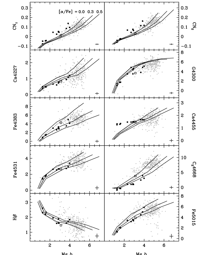
Figure 2: ${\rm Mg}\,b$ index versus the other 20 Lick indices. Solid lines are the models of this paper with constant age (12 Gyr), constant $\alpha/{\rm Fe}$, and for the metallicity range $-2.25\leq[Z/{\rm H}]\leq 0.67$. Three models with $[\alpha/{\rm Fe}]=0.0,\ 0.3,\ 0.5$ are shown. Models with solar abundance ratios ($[\alpha/{\rm Fe}]=0.0$) and models with $[\alpha/{\rm Fe}]=0.5$ are those with the lowest and highest ${\rm Mg}\,b$ indices, respectively. The dotted lines are our base SSP models (Maraston, 1998). Filled squares are globular cluster data, the open square is the integrated Bulge light from Puzia et al. (2002), small grey dots are the Lick data of giant elliptical galaxies from Trager et al. (1998). Errorbars indicate typical errors of the globular cluster data.

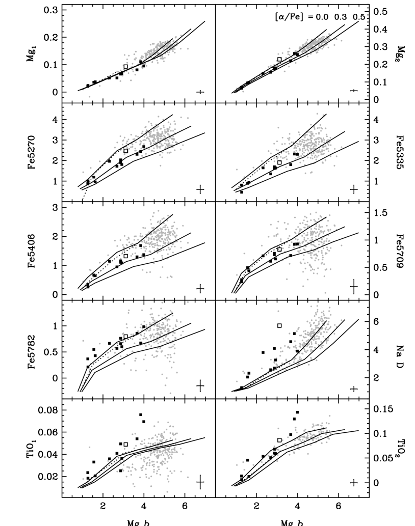
Figure 3: continued

From high-resolution stellar spectroscopy it is known that globular clusters in both the halo and the Bulge of our Galaxy are $\alpha/{\rm Fe}$ enhanced with the typical values $[\alpha/{\rm Fe}]\approx 0.3\pm 0.1$ dex (Barbuy et al. 1999, Cohen et al. 1999, Carretta et al. 2001, Coelho et al. 2001, Origlia, Rich & Castro 2002, and compilations by Carney 1996, and Salaris & Cassisi 1996). Hence, the observed Lick indices of globular clusters should be matched by SSP models with $t\approx 12$ Gyr (see above) and $[\alpha/{\rm Fe}]\approx 0.3$.

The comparison is shown in Fig. 2, in which we plot the ${\rm Mg}\,b$ index versus the other 20 Lick indices. The indices are arranged according to increasing wavelength. Filled squares are globular cluster data (Puzia et al., 2002), solid lines are the new SSP models presented here with constant age (12 Gyr) and constant $\alpha/{\rm Fe}$ ratio. All models cover the metallicity range $-2.25\leq[Z/{\rm H}]\leq 0.67$. The three lines are models with the abundance ratios $[\alpha/{\rm Fe}]=0.0,\ 0.3,\ 0.5$ dex. Models with solar abundance ratios ($[\alpha/{\rm Fe}]=0.0$) and models with $[\alpha/{\rm Fe}]=0.5$ are those with the lowest and highest ${\rm Mg}\,b$ indices, respectively. The dotted lines are the base SSP model. For well calibrated indices, the squares (globular cluster data) should scatter about the middle line (model with $[\alpha/{\rm Fe}]=0.3$). The open square is the integrated Bulge light (Puzia et al., 2002), small grey symbols are the Lick data of giant elliptical galaxies from Trager et al. (1998).

3.1.1 The $\alpha/{\rm Fe}$ bias in standard models

The standard models are shown as dotted lines in Fig. 2. As their $\alpha/{\rm Fe}$ bias is $[\alpha/{\rm Fe}]\approx 0.3$ at the lowest metallicity (see Table 3), this biased model (dotted line) deviates clearly from the $[\alpha/{\rm Fe}]=0$ model and coincides with the $[\alpha/{\rm Fe}]=0.3$ model (middle solid line). Indeed, as shown in Maraston et al. (2002), because of the $\alpha/{\rm Fe}$ bias the base model matches the Lick data of the metal-poor globular clusters. At solar metallicity and above, there is no bias in the standard model (Table 3), so that the dotted lines and the $[\alpha/{\rm Fe}]=0.0$ model (solid line with the lowest ${\rm Mg}\,b$) are indistinguishable for $[Z/{\rm H}]\geq 0$. This pattern is present throughout all panels in Fig. 2.

3.1.2 Sensitivity to Fe-peak elements

As emphasized in T00, and explained at the beginning of Section 2.2, the enhancement of the $\alpha/{\rm Fe}$ ratio at fixed metallicity is produced essentially by a depletion of the Fe abundance (see also Buzzoni et al. 1992), and only by a slight increase of the $\alpha$-element abundances. The reason is that Fe-peak elements are by far less abundant than oxygen and the other $\alpha$-elements. As a consequence, only indices that are sensitive to Fe-peak element abundance variations respond to $\alpha/{\rm Fe}$ ratio changes at fixed metallicity. ${\rm Mg}\,b$, for instance, anti-correlates with Fe abundance (TB95), and therefore increases with increasing $\alpha/{\rm Fe}$.

Ca4227, instead, correlates with both Ca and Fe abundance (TB95). As the depletion of iron dominates the $\alpha/{\rm Fe}$ enhanced model, Ca4227 actually decreases with increasing $\alpha/{\rm Fe}$, although the element calcium belongs to the enhanced group in our models. The indices ${\rm CN}_{1}$ and ${\rm CN}_{2}$ correlate with $\alpha/{\rm Fe}$, also mainly because of their sensitivity to Fe-peak element abundances.

3.1.3 Discussion on individual indices

Figure 4: Models in which carbon is enhanced by 0.1 dex (left-hand panels) and in which nitrogen is enhanced by 0.5 dex (right-hand panels). Only carbon and nitrogen sensitive indices are shown. Line-styles and symbols like in Fig. 2.

${\rm CN}_{1}$,${\rm CN}_{2}$.—The models clearly predict too low index values at all metallicities, in particular for ${\rm CN}_{1}$, although both indices respond positively to changes in the $\alpha/{\rm Fe}$ ratios. Such relatively strong CN absorption features have also been observed for extragalactic globular clusters in M 31 (Burstein et al., 1984) and NGC 3115 (Kuntschner et al., 2002). As shown in Maraston et al. (2002), the mismatch between models and data is already present in the standard SSP model (dotted lines), thus cannot be attributed to a failure of the TB95 index responses. Moreover, the integrated light of the galactic Bulge (open squares) does not have such strong CN absorption features.

It has been suggested by D’Antona, Gratton & Chieffi (1983) and Renzini (1983), that stars in globular clusters may accrete carbon and/or nitrogen enriched ejecta from the surrounding AGB stars (Renzini & Voli, 1981). Indeed ${\rm CN}_{1}$ and ${\rm CN}_{2}$ are very sensitive to carbon and to nitrogen abundances (TB95). To test this option quantitatively, we computed additional models enhancing separately the abundances of C and N. The resulting models for the indices ${\rm CN}_{1}$, ${\rm CN}_{2}$, Ca4227, ${\rm C}_{2}$4668, and ${\rm Mg}_{1}$ are shown in Fig. 4. The remaining Lick indices (except G4300) are not affected by carbon and nitrogen abundance changes.

An increase of the carbon abundance by 30 per cent is sufficient to obtain an excellent match of the ${\rm CN}_{1}$ and ${\rm CN}_{2}$ data (left-hand, top panels in Fig. 4). However, also ${\rm C}_{2}$4668 and ${\rm Mg}_{1}$ strongly correlate with the element carbon, so that these indices are not reproduced any more by the models with enhanced carbon abundance (left-hand middle panels in Fig. 4). It is not possible to match simultaneously the four indices ${\rm CN}_{1}$, ${\rm CN}_{2}$, ${\rm C}_{2}$4668, and ${\rm Mg}_{1}$. Assuming that the index responses by TB95 are correct, we can rule out that a significant enhancement of the carbon abundance produces the ${\rm CN}_{1}$ and ${\rm CN}_{2}$ indices of globular clusters (see also Worthey, 1998).

Increasing the nitrogen abundance by a factor 3 with respect to the $\alpha$-elements ($[\alpha/{\rm N}]=-0.5$), instead, the indices ${\rm CN}_{1}$ and ${\rm CN}_{2}$ are well reproduced, without destroying the match to the other indices, as the latter are almost insensitive to nitrogen abundance (right-hand panels in Fig. 4, Table 1). Based on the TB95 calculations, already Worthey (1998) argued that an enhancement of nitrogen rather than carbon is required to explain the CN-absorption in globular cluster stars. The model calculations of this paper now allow us to quantify this conclusion. We show that nitrogen needs to be enhanced in globular cluster stars by 0.5 dex (factor 3). This is consistent with the results from Origlia et al. (2002), who find nitrogen to be enhanced by a factor $\approx 2$ in stars in NGC 6553, while carbon is not enhanced. It should be emphasized again that the CN features of the Bulge light, instead, are perfectly reproduced by the models without extra-enhancement of nitrogen.

Ca4227.–The absorption index Ca4227 is predicted slightly too high by the models. Interestingly, Ca4227 is the only index besides ${\rm CN}_{1}$ and ${\rm CN}_{2}$ which is considerably affected by changes of carbon and nitrogen abundances. Its line-strength is anti-correlated with CN abundances (TB95), so that the poor match of the globular cluster data in Fig. 2 is improved with the CN-enhanced models shown in the bottom panels of Fig. 4. Taking the enhancement of nitrogen into account, our $\alpha/{\rm Fe}$ enhanced models with $[{\rm Ca}/{\rm Fe}]=[\alpha/{\rm Fe}]$, provide a good fit to the globular cluster data, including the metal-rich clusters NGC 6528 and NGC 6553. This indicates that the latter do not exhibit any anomalies in calcium abundance, i.e. their Ca/Fe ratio are enhanced like the other $\alpha$-element/Fe ratios. This result agrees with element abundances derived for single stars in these clusters (Carretta et al., 2001; Origlia et al., 2002), even though the latter are still controversial. Barbuy and coworkers (B. Barbuy, 2002, private communication) measure $[{\rm Mg}/{\rm Fe}]=0.3$ but $[{\rm Ca}/{\rm Fe}]=0.0$ in a clump star of NGC 6528, which would imply a Ca underabundance in that cluster.

Motivated by the realization that elliptical galaxies have weaker Ca4227 indices than predicted by standard SSP models (Vazdekis et al., 1997; Trager et al., 1998), we additionally computed models of Ca4227 with variable $\alpha/{\rm Ca}$ ratios (Table 1). The application of these models and the derivation of $\alpha/{\rm Ca}$ ratios for elliptical galaxies is presented in an accompanying paper (D. Thomas et al., in preparation).

G4300.–This index is mainly sensitive to carbon and oxygen abundances, only little to Fe abundance (TB95). It responds therefore only marginally to the $\alpha/{\rm Fe}$ ratio changes, as enhanced $\alpha/{\rm Fe}$ ratios are not caused by $\alpha$-element enhancement, but by Fe reduction. At high metallicities, it is even less sensitive to total metallicity than ${\rm H}\beta$ (see also TB95). The calibration of the models with the globular cluster data is not convincing.

Fe4383.–This index is very sensitive to Fe abundance, hence $\alpha/{\rm Fe}$ ratios. The models provide an excellent fit to the data, so that Fe4383 is well calibrated and represents a promising (blue) alternative to the classic indices Fe5270 and Fe5335.

Ca4455.–As emphasized by TB95, despite its name Ca4455 is insensitive to Ca abundance, while Fe and Cr, both elements of the depressed group, are the dominant contributors to this index. As Ca4455 is correlated to Cr, but anti-correlated to Fe abundance, however, it responds hardly to $\alpha/{\rm Fe}$ ratios changes. The globular cluster data and the model predictions are not compatible as already shown in case of the base model (Maraston et al., 2002). It is more likely that this mismatch originates from an offset of the globular cluster data from the Lick system (see Maraston et al., 2002), because these data seem also incompatible with the Lick galaxy data of Trager et al. (1998, small grey symbols). The index Ca4455 is therefore not a useful abundance indicator.

Fe4531.–This index is reasonably well calibrated, but it is less sensitive to Fe abundance and $\alpha/{\rm Fe}$ ratios than Fe4383.

${\rm C}_{2}$4668.–Formerly called Fe4668, this index has been renamed, because it is most sensitive to carbon abundance (TB95). As carbon is kept fixed in our models, ${\rm C}_{2}$4668 decreases only slightly with increasing $\alpha/{\rm Fe}$. Owing to the poor match between models and globular cluster data, this index is not well suited for element abundance studies. Assigning carbon to the depressed group, does not improve the match between data and models, and provokes inconsistencies with the otherwise well calibrated indices ${\rm Mg}_{1}$, ${\rm CN}_{1}$, and ${\rm CN}_{2}$.

${\rm H}\beta$.–The Balmer absorption index is well calibrated. It increases mildly with increasing $\alpha/{\rm Fe}$. The increase of Balmer absorption in globular clusters with decreasing metallicity is very well reproduced by our models (see also Maraston & Thomas, 2000). This strong Balmer absorption at old ages and low metallicities stems from the development of warm horizontal branches owing to mass loss on the Red Giant Branch. As shown in Maraston et al. (2002), the slightly lower ${\rm H}\beta$ values of the two globular clusters at intermediate metallicity (${\rm Mg}\,b\approx 2.8$) can be easily reproduced by models with reduced mass loss along the red giant branch, in good agreement with their observed red horizontal branch morphologies. The models used here have blue horizontal branches at metallicities below $[Z/{\rm H}]\sim-1$.

Fe5015.–Although TB95 produce only a poor fit of this index, our models are in good agreement with the globular cluster data. As Fe5015 is only little sensitive to $\alpha/{\rm Fe}$ ratios, however, it is less recommendable for abundance ratio studies than Fe4383.

${\rm Mg}_{1}$,${\rm Mg}_{2}$.–It is very reassuring that all three Mg-indices ${\rm Mg}_{1}$, ${\rm Mg}_{2}$, and ${\rm Mg}\,b$ respond very similarly to $\alpha/{\rm Fe}$ ratio changes. The models plotted in Fig. 2 are therefore highly degenerate. The globular cluster data are well reproduced. Among the three indices, ${\rm Mg}_{2}$ turns out to be least, ${\rm Mg}\,b$ to be most sensitive to $\alpha/{\rm Fe}$.

Fe5270,Fe5335.–These are the classical indicators for Fe abundance. They are perfectly matched by our models. Fe5335 is somewhat more sensitive to $\alpha/{\rm Fe}$.

Fe5406.–This index is very similar to Fe5270 and Fe5335. Although the $\alpha/{\rm Fe}$ enhanced models predict slightly lower Fe5406 values than suggested by the data, this index is still reasonably well calibrated.

Fe5709.–The match between models and data is excellent. However, Fe5709 responds less strongly to $\alpha/{\rm Fe}$ because of its weaker sensitivity to Fe abundance (TB95).

Fe5782.–For this index, the match between models and globular cluster data is very poor. Different from the situation of Ca4455, it is hard to assess if the globular cluster data are compatible with the Lick galaxy measurements of Trager et al. (1998). The standard SSP models (dotted line), which are perfectly compatible with the Worthey (1994) models, clearly predict too low Fe5782 indices. A miscalibration of the fitting function therefore may also be a possible explanation for the mismatch between models and data (Maraston et al., 2002).

Na D.–Similar to Fe5782, the standard SSP model gives lower index values than suggested by the observational data, in accordance with the Worthey (1994) models. An unrealisticly large sensitivity of the index to the $\alpha/{\rm Fe}$ ratio would be required to lift the models on the data. Most likely, the strong NaD absorption is caused by Na absorption in interstellar material of the Galactic disc. Indeed, there is the clear trend that the clusters in the sample that are closer to the Galactic plane have higher NaD relative to their ${\rm Mg}\,b$ indices. This high sensitivity of the NaD index to interstellar absorption severely hampers its usefulness for stellar population studies.

${\rm TiO}_{1}$,${\rm TiO}_{2}$.–Both indices appear badly calibrated, although the agreement between models and data for ${\rm TiO}_{2}$ is still acceptable. As discussed in Puzia et al. (2002), the most metal-rich clusters NGC 6528 and NGC 6553 show very strong ${\rm TiO}_{2}$ absorption because of their extremely cool Red Giant Branches, in accordance with the strong bending observed in color-magnitude diagrams (Ortolani, Barbuy & Bica, 1991; Cohen & Sleeper, 1995).

3.1.4 Measuring $\alpha/{\rm Fe}$ from ${\rm Mg}\,b$/$\langle{\rm Fe}\rangle$

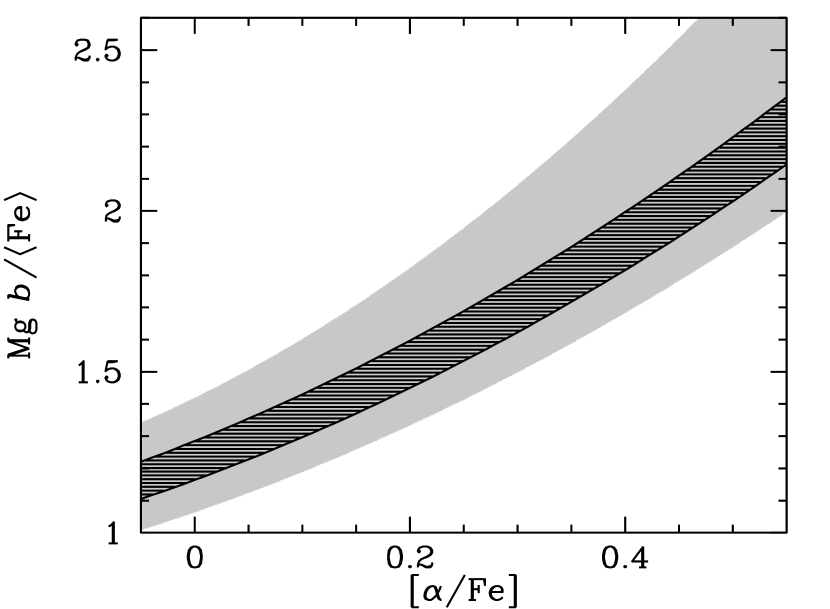
Figure 5: Lick index ratio ${\rm Mg}\,b$/$\langle{\rm Fe}\rangle$ as a function of element abundance ratio $\alpha/{\rm Fe}$. The dark hashed area are models covering metallicities $-1.35\leq[Z/{\rm H}]\leq 0.35$ and ages from 8 to 15 Gyr. The light-grey area are models with the same metallicities but the larger age range $3\leq t\leq 15$ Gyr.

The models provided here allow for the derivation of $\alpha/{\rm Fe}$ element ratios from the Lick indices like ${\rm Mg}\,b$ and $\langle{\rm Fe}\rangle$. In the following, we show how the index ratio ${\rm Mg}\,b$/$\langle{\rm Fe}\rangle$ can be used to obtain an estimate of the element ratio $\alpha/{\rm Fe}$. For this purpose, in Fig. 5 we plot ${\rm Mg}\,b$/$\langle{\rm Fe}\rangle$ as a function of $\alpha/{\rm Fe}$. As ${\rm Mg}\,b$/$\langle{\rm Fe}\rangle$ depends not only on $\alpha/{\rm Fe}$ but also on age and metallicity, we show the areas covered by models with a range in ages and metallicities. The dark shaded area are models covering metallicities $-1.35\leq[Z/{\rm H}]\leq 0.35$ and ages from 8 to 15 Gyr. The light-grey area are models with the same metallicities but the larger age range $3\leq t\leq 15$ Gyr.

For old populations (ages above $\sim 8$ Gyr), the relation between ${\rm Mg}\,b$/$\langle{\rm Fe}\rangle$ and $\alpha/{\rm Fe}$ is reasonably well defined independent of age and metallicity. In this case, Fig. 5 allows to read off directly the $\alpha/{\rm Fe}$ element ratio $\pm 0.04$ dex from the measured index ratio ${\rm Mg}\,b$/$\langle{\rm Fe}\rangle$.

3.1.5 $\alpha/{\rm Fe}$ enhanced stellar evolutionary tracks

In the models presented here, solar-scaled stellar tracks are adopted. The impact on Lick indices due to $\alpha/{\rm Fe}$ enhancement is accounted for through a modification of the stellar absorption line-strengths (see Section 2). A fully self-consistent $\alpha/{\rm Fe}$ enhanced SSP model should in principle use $\alpha/{\rm Fe}$ enhanced stellar evolutionary tracks, because the element abundance variations in a star affect also the star’s evolution and the opacities in the stellar atmosphere, hence the effective temperature. We are planning in future to compute SSP models with $\alpha/{\rm Fe}$ enhanced tracks that are based—for reasons of self-consistency—on the same input tracks (Cassisi et al., 1997) as the present models.

To assess the impact of $\alpha/{\rm Fe}$ in the stellar evolutionary tracks, Maraston et al. (2002) compute standard models with the solar-scaled and the $\alpha/{\rm Fe}$ enhanced tracks from Salasnich et al. (2000). As the $\alpha/{\rm Fe}$ enhanced tracks are hotter than the solar-scaled ones (Salasnich et al., 2000), their inclusion in the stellar population model leads to slightly weaker metallic indices (i.e. ${\rm Mg}\,b$, $\langle{\rm Fe}\rangle$ etc.) and stronger Balmer line indices (${\rm H}\beta$) for the same age and metallicity (Fig. 5 in Maraston et al., 2002). The decrease of ${\rm Mg}\,b$ and $\langle{\rm Fe}\rangle$ are comparable, so that the additional inclusion of $\alpha/{\rm Fe}$ enhanced tracks has only a minor effect on the ${\rm Mg}\,b$-$\langle{\rm Fe}\rangle$ plane, and therefore has no significant impact on the derivation of $\alpha/{\rm Fe}$ ratios. This issue is explored in detail in an accompanying paper (Thomas & Maraston, 2002).

3.1.6 Summary

To briefly summarize, the classical indices ${\rm Mg}_{1}$, ${\rm Mg}_{2}$, ${\rm Mg}\,b$ and the blue indices ${\rm CN}_{1}$ and ${\rm CN}_{2}$ increase with increasing $\alpha/{\rm Fe}$ ratio, in particular the latter owing to an anti-correlation with Fe abundance. With the caveat that ${\rm CN}_{1}$ and ${\rm CN}_{2}$ are very sensitive to C and N abundances, these two can be regarded complementary to the indices Mg₁, Mg₂, ${\rm Mg}\,b$. Besides the intensively studied iron indices Fe5270 and Fe5335, the indices Fe4383, Fe4531, Fe5015, and Fe5709 are good representatives of Fe-peak element abundances. The indices G4300, Ca4455, ${\rm C}_{2}$4668, Fe5782, Na D, ${\rm TiO}_{1}$, instead, are poorly calibrated and do not provide valuable information on abundance ratios. Ca4227, ${\rm H}\beta$, Fe5406 and ${\rm TiO}_{2}$ cannot be assigned to any of these three categories.

${\rm H}\beta$ is only little sensitive to element abundance variations, and is well calibrated. Ca4227 is mainly sensitive to Ca and N abundances. This index, and the indices ${\rm CN}_{1}$ and ${\rm CN}_{2}$, require an additional enhancement of nitrogen abundance with respect to the other $\alpha$-elements by a factor 3 ($[\alpha/{\rm N}]=-0.5$), in order to fit the globular cluster data.

Concluding, the combination of the blue indices ${\rm CN}_{1}$, ${\rm CN}_{2}$ and Fe4383 may be best suited to estimate $\alpha/{\rm Fe}$ ratios of objects at redshifts $z\sim 1$.

3.2 Metallicities

3.2.1 The globular cluster metallicity scale

In this section we compare the total metallicities [$Z/{\rm H}$] derived here for the galactic globular cluster sample with the metallicities given in the Harris (1996) catalog, which are based on the Zinn & West (1984, hereafter ZW84) scale. We add the data of the globular cluster 47 Tuc from Maraston et al. (2002). For the metal-rich bulge cluster NGC 6553 we adopt the more recent measurements of single star abundances by Barbuy et al. (1999), who find—in good agreement with Origlia et al. (2002)—solar total metallicity.

Figure 6: Zinn & West (1984) metallicity (Harris, 1996) vs. the total metallicity [$Z/{\rm H}$] derived in this paper for galactic globular clusters from Puzia et al. (2002). [$Z/{\rm H}$] is determined from the indices ${\rm Mg}\,b$ and Fe5270, using our SSP models with fixed age $t=12$ Gyr. We assume an error of 0.2 dex for the ZW84 metallicities.

ZW84 metallicities are usually referred to as [Fe/H]. As we actually aim at calibrating our SSP models, in which we distinguish between total metallicity [$Z/{\rm H}$] and iron abundance [${\rm Fe}/{\rm H}$], at this point it is crucial to understand, if the ZW84 metallicity scale traces total metallicity or iron abundance. It is important to remember, that the ZW84 scale at $[{\rm Fe}/{\rm H}]>-1.5$ is based on measurements by Cohen (1983) of the pseudo-equivalent widths for the Mg triplet near 5175 Å, and the 5270 and 5206 Å Fe blends. She derives the metallicity from averaging the Mg and Fe equivalent widths. These metallicities are then used by ZW84 to set up a globular cluster metallicity scale. The average of Mg and Fe line kills information on $\alpha/{\rm Fe}$ ratios and is likely to be close to the total metallicity. This strongly suggests that the ZW84 metallicity scale traces total metallicity rather than iron abundance at $[Z/{\rm H}]\ga-1.5$. We suggest that the ZW84 metallicities should better be written as [$Z/{\rm H}$] instead of [Fe/H], in order to avoid confusion.

We determine [$Z/{\rm H}$] from the Lick indices ${\rm Mg}\,b$ and Fe5270, using our SSP models with fixed age $t=12$ Gyr. Note that using alternatively the indices ${\rm Mg}_{2}$ and/or Fe5335 yields perfectly consistent results. Fig. 6 shows that our derived total metallicities [$Z/{\rm H}$] are in excellent agreement with the ZW84 metallicity scale. This result is highly reassuring but not unexpected, as we derive metallicities from exactly the same lines (Mg triplet at 5157 Å and Fe blend at 5270 Å) as Cohen (1983), even though from integrated light and at the much lower Lick resolution ($\sim 8$ Å).

The iron abundance [Fe/H] can be obtained through the following scaling (see Section 2.2, Eqn. 4),

$$[{\rm Fe}/{\rm H}]=[Z/{\rm H}]-0.94\ [\alpha/{\rm Fe}]$$

and is lower than [$Z/{\rm H}$] for super-solar $\alpha/{\rm Fe}$ ratios. The [$Z/{\rm H}$] and [$\alpha/{\rm Fe}$] ratios derived here for the globular cluster sample are listed in Table 4. The iron abundances of all the globulars considered here are lower than the total metallicity by typically $\sim 0.3$ dex. Our measured [Fe/H] are therefore systematically lower by this value than the ZW84 metallicities, reinforcing the interpretation that the ZW84 scale implies total metallicity.

Table 4: Derived element abundances

Name	[$Z/{\rm H}$]	[$\alpha/{\rm Fe}$]
NGC 6528	$-0.14\ \pm 0.19$	$0.31\ \pm 0.32$
NGC 6553	$-0.05\ \pm 0.07$	$0.23\ \pm 0.12$
NGC 5927	$-0.21\ \pm 0.11$	$0.35\ \pm 0.21$
NGC 6388	$-0.65\ \pm 0.03$	$0.08\ \pm 0.04$
NGC 6624	$-0.52\ \pm 0.08$	$0.33\ \pm 0.09$
NGC 6218	$-1.59\ \pm 0.43$	$0.24\ \pm 0.45$
NGC 6441	$-0.46\ \pm 0.07$	$0.26\ \pm 0.07$
NGC 6626	$-1.21\ \pm 0.10$	$0.14\ \pm 0.21$
NGC 6284	$-1.29\ \pm 0.15$	$0.38\ \pm 0.24$
NGC 6356	$-0.55\ \pm 0.08$	$0.40\ \pm 0.10$
NGC 6637	$-0.65\ \pm 0.07$	$0.35\ \pm 0.08$
NGC 6981	$-1.41\ \pm 0.30$	$0.09\ \pm 0.35$
47 Tuc	$-0.83\ \pm 0.23$	$0.19\ \pm 0.35$

Based on high resolution spectroscopy of individual stars in globular clusters, Carretta & Gratton (1997) suggest a revision of the classical ZW84 scale to essentially higher metallicities. The shift is of the order 0.2 dex, which leads to a clear disagreement between the metallicities derived here from Lick indices and the metallicity scale of Carretta & Gratton (1997). The same discrepancy emerges from considering integrated colors of globular clusters. Maraston (2000) show that SSP models using reasonable ages ($\ga 9$ Gyr) and the Carretta & Gratton (1997) metallicities of globular clusters predict $B\!-\!V$ colors that are too red compared to the observed values. With the ZW84 metallicities, instead, excellent agreement between SSP model prediction and observation is found. Caputo & Cassisi (2002) come to the same conclusion comparing isochrones with observed color-magnitude diagrams of globular clusters.

Interestingly, in contrast to Cohen (1983), Carretta & Gratton (1997) measure ’metallicity’ exclusively from Fe line features, so that their values should rather be iron abundances than total metallicities. Taking this into account, the discrepancy to the metallicities derived from isochrones and SSP models gets even more severe (see Fig. 8 in Maraston et al., 2002). Barbuy (2000) suggests that Carretta & Gratton (1997) may tend to overestimate element abundances and metallicities because of a hotter temperature scale.

A comparison between the metallicities of globular clusters derived from Lick indices and the ZW84 metallicity scale has also been carried out by Cohen, Blakeslee & Ryzhov (1998). They used Worthey (1994)’s SSP models to fit simultaneously by $\chi^{2}$ minimization the indices ${\rm Mg}\,b$, NaD, Fe5270, and Fe5335 measured for globular clusters including also the metal-rich bulge cluster NGC 6528. The authors did not find a satisfying consistency between their derived metallicities and the ZW84 scale. They had to introduce a scaling between ZW84 and their derived metallicities, as they over-predicted metallicities for the more metal-rich clusters. This may partly be due to the higher Fe indices measured (see Puzia et al., 2002), partly due to the fact that Worthey (1994)’s SSP models do not include $\alpha/{\rm Fe}$ abundance effects.

Concluding, we would like to emphasize again that metallicity determinations from colors and Lick indices with the models of this paper are both in excellent agreement with the ZW84 metallicity scale. This highly encouraging self-consistency is also found by Kuntschner et al. (2002), who derive—with the models of this paper—the same metallicities of globular clusters in the elliptical galaxy NGC 3115 from the Lick indices ${\rm Mg}\,b$ and $\langle{\rm Fe}\rangle$, and $V\!-\!I$ colors.

3.2.2 Brodie & Huchra’s metallicity calibration

Measuring line indices on galactic and M31 globular cluster spectra, Brodie & Huchra (1990) derived a linear correlation between ${\rm Mg}_{2}$ index and ZW84 metallicity. For a comparison of our derived metallicities [$Z/{\rm H}$] with this calibration, in Fig. 7 we show [$Z/{\rm H}$] of the globular cluster sample versus ${\rm Mg}_{2}$, and over-plot as a solid line the linear relation derived by Brodie & Huchra (1990). The dotted line is our SSP model with age $t=12$ Gyr and $[\alpha/{\rm Fe}]=0.3$.

Figure 7: Total metallicity [$Z/{\rm H}$] versus ${\rm Mg}_{2}$ index. The circles are galactic globular clusters (Puzia et al., 2002). [$Z/{\rm H}$] is determined from the indices ${\rm Mg}\,b$ and Fe5270, using the SSP models of this paper with fixed age $t=12$ Gyr (see also Fig. 6). The solid line is the metallicity calibration by Brodie & Huchra (1990). The dotted line is the SSP model of this paper with fixed age $t=12$ Gyr and $[\alpha/{\rm Fe}]=0.3$.

Although reassuring, the excellent agreement does certainly not come as a surprise, as Brodie & Huchra (1990) derived their fit on the basis of ZW84 metallicities, which are perfectly consistent with our [$Z/{\rm H}$] values (Fig. 6). More interesting are the two most metal-rich clusters NGC 6528 and NGC 6553, which exhibit significantly stronger ${\rm Mg}_{2}$ than predicted by the Brodie & Huchra (1990) calibration. These clusters have almost solar metallicities, while the Brodie & Huchra (1990) calibration is based on globular clusters with $[Z/{\rm H}]<-0.5$. A non-linear increase of ${\rm Mg}_{2}$ with increasing total metallicity at metallicities $[Z/{\rm H}]>-0.5$, instead, is suggested by the data and consistently predicted by our SSP models (dotted line).

3.2.3 Tracing metallicity independent of $\alpha/{\rm Fe}$

The new SSP models with variable $\alpha/{\rm Fe}$ ratio allow for an unambiguous derivation of total metallicity and $\alpha/{\rm Fe}$ ratio simultaneously, free from any $\alpha/{\rm Fe}$ bias. Still, it would be useful to find an index that is mainly a tracer of total metallicity independent of the $\alpha/{\rm Fe}$ ratio. González (1993) suggested that averaging Mg and Fe indices may yield such a metallicity indicator, and defined the index

$$[{\rm MgFe}]=\sqrt{{\rm Mg}\,b\cdot\langle{\rm Fe}\rangle}$$

with

$$\langle{\rm Fe}\rangle=\frac{1}{2}\ ({\rm Fe5270}+{\rm Fe5335})\ .$$

In Fig. 8 we plot the Lick indices ${\rm Mg}\,b$ and $\langle{\rm Fe}\rangle$ of our SSP models as functions of $\alpha/{\rm Fe}$ ratio at fixed total metallicity. Models with age 12 Gyr and solar metallicity are shown. ${\rm Mg}\,b$ increases and $\langle{\rm Fe}\rangle$ decreases with increasing $\alpha/{\rm Fe}$. The index [MgFe] as defined by González (1993) is the dotted line. Although being only very little sensitive to $\alpha/{\rm Fe}$, still [MgFe] slightly decreases with increasing $\alpha/{\rm Fe}$.

Figure 8: Lick indices as function of $\alpha/{\rm Fe}$ ratio at fixed total metallicity. Plotted are the indices ${\rm Mg}\,b$, $\langle{\rm Fe}\rangle=\frac{1}{2}({\rm Fe5270}+{\rm Fe5335})$, and $[{\rm MgFe}]^{\prime}\equiv\sqrt{{\rm Mg}\,b\ (0.72\cdot{\rm Fe5270}+0.28\cdot{\rm Fe5335})}$ of 12 Gyr old SSP models with solar metallicity. The dotted line is the index [MgFe] as defined by González (1993).

From Table 2 we know that Fe5270 responds less to $\alpha/{\rm Fe}$ ratio changes than Fe5335. Decreasing the weight of Fe5335 in the definition of [MgFe] thus helps to remove the sensitivity to $\alpha/{\rm Fe}$. We therefore slightly modify the definition of [MgFe] and define the new index

$${\rm[MgFe]}^{\prime}\equiv\sqrt{{\rm Mg}\,b\ (0.72\cdot{\rm Fe5270}+0.28\cdot{\rm Fe5335})}\ .$$ (12)

In Fig. 8 it is shown that ${\rm[MgFe]}^{\prime}$ is indeed completely independent of $\alpha/{\rm Fe}$. We note that this behaviour is almost independent of the adopted age and metallicity. Therefore [MgFe]^′ serves best as a tracer of the total metallicity of stellar populations.

4 Conclusions

We present a comprehensive set of new generation stellar population models of Lick absorption line indices, which for the first time include abundance ratios different from solar. We computed the 21 Lick indices ${\rm CN}_{1}$, ${\rm CN}_{2}$, Ca4227, G4300, Fe4383, Ca4455, Fe4531, ${\rm C}_{2}$4668, ${\rm H}\beta$, Fe5015, ${\rm Mg}_{1}$, ${\rm Mg}_{2}$, ${\rm Mg}\,b$, Fe5270, Fe5335, Fe5406, Fe5709, Fe5782, Na D, ${\rm TiO}_{1}$, and ${\rm TiO}_{2}$ in the wavelength range $4000\la\lambda\la 6500$ Å. Models are provided with: $[\alpha/{\rm Fe}]=0.0,\>0.3,\>0.5$, $[\alpha/{\rm Ca}]=-0.1,\>0.0,\>0.2,\>0.5$, and $[\alpha/{\rm N}]=-0.5,\>0.0$; ages from 1 to 15 Gyr; total metallicities from 1/200 to 3.5 solar ($-2.25\leq[Z/{\rm H}]\leq 0.67$).

The models are based on the evolutionary synthesis technique described in Maraston (1998). The $\alpha/{\rm Fe}$ enhanced mixtures are obtained by increasing the abundances of $\alpha$-group elements and by decreasing the abundances of the Fe-peak elements, such that total metallicity is conserved. The impact from these element abundance variations on the absorption line indices is taken from Tripicco & Bell (1995), using an extension of the method introduced by Trager et al. (2000). Most importantly, we take into account that the empirical stellar libraries used to compute model indices follow the chemical enrichment history of the Milky Way, and are therefore biased towards super-solar $\alpha/{\rm Fe}$ ratios at sub-solar metallicities. We corrected for this bias, so that the models presented here have well-defined $\alpha/{\rm Fe}$ ratios at all metallicities.

We take particular care at calibrating the models with galactic globular clusters, for which ages, metallicities, and element abundance ratios are known from independent sources. Our $\alpha/{\rm Fe}$ enhanced models with $[\alpha/{\rm Fe}]=0.3$ (and 12 Gyr age) perfectly reproduce the positions of the globular cluster data in the ${\rm Mg}\,b$-$\langle{\rm Fe}\rangle$ diagram up to solar metallicities (see also Maraston et al., 2002). The total metallicities for the sample clusters that we derive from these indices are in excellent agreement with the Zinn & West (1984) metallicity scale. We point out that the latter most likely reflects total metallicity rather than iron abundance, because it is obtained essentially by averaging the abundances derived from the Mg triplet near 5175 Å and the Fe blend at 5270 Å (Cohen, 1983; Zinn & West, 1984). This aspect needs to be emphasized, as with the $\alpha/{\rm Fe}$ enhanced models we are now in the position to distinguish total metallicity [$Z/{\rm H}$] and iron abundance [Fe/H].

By means of our calibrated $\alpha/{\rm Fe}$ enhanced models, we confirm that the index [MgFe], suggested by González (1993) to balance $\alpha/{\rm Fe}$ ratio effects, is almost independent of $\alpha/{\rm Fe}$. As it modestly decreases with increasing $\alpha/{\rm Fe}$, however, we define the slightly modified index

$${\rm[MgFe]}^{\prime}\equiv\sqrt{{\rm Mg}\,b\ (0.72\cdot{\rm Fe5270}+0.28\cdot{\rm Fe5335})}\ ,$$

which is completely independent of $\alpha/{\rm Fe}$, and hence an even better tracer of total metallicity. We further show that the linear correlation between ${\rm Mg}_{2}$ and metallicity at old ages derived empirically by Brodie & Huchra (1990) is valid up to $\sim 1/3$ solar metallicity, but underpredicts ${\rm Mg}_{2}$ indices at metallicities above that threshold.

It turns out to be hard to find indices that correlate with $\alpha/{\rm Fe}$ as well as the intensively studied indices ${\rm Mg}_{1}$, ${\rm Mg}_{2}$, and ${\rm Mg}\,b$. Promising alternatives are the blue indices ${\rm CN}_{1}$ and ${\rm CN}_{2}$ that also increase with increasing $\alpha/{\rm Fe}$ ratio, mainly because of an anti-correlation with Fe abundance. With the caveat that ${\rm CN}_{1}$ and ${\rm CN}_{2}$ are additionally sensitive to C and N abundances, they can be regarded to be complementary to the indices ${\rm Mg}_{1}$, ${\rm Mg}_{2}$, and ${\rm Mg}\,b$. Alternatives to the iron indices Fe5270 and Fe5335, the strengths of which decrease with increasing $\alpha/{\rm Fe}$ ratio, are easier to find. The best cases are the indices Fe4383, Fe4531, Fe5015, and Fe5709.

The indices ${\rm CN}_{1}$, ${\rm CN}_{2}$, and Ca4227 of globular clusters are very interesting, particular cases. We find that the relatively strong CN features observed in globular clusters require models in which nitrogen is enhanced by a factor three relative to the $\alpha$-elements, hence $[\alpha/{\rm N}]=-0.5$. This is in agreement with early suggestions by D’Antona et al. (1983) and Renzini (1983), that stars in globular clusters may accrete carbon and/or nitrogen enriched ejecta from the surrounding AGB stars (Renzini & Voli, 1981). The good calibration of other indices like ${\rm Mg}_{1}$, ${\rm Mg}\,b$ or $\langle{\rm Fe}\rangle$ is not affected by a variation of the $\alpha/{\rm N}$ ratio, as these indices are not sensitive to nitrogen abundance. We note that an enhancement of carbon abundance, instead, would lead to serious inconsistencies with ${\rm Mg}_{1}$. Interestingly, also Ca4227 is sensitive to nitrogen abundance, and the globular cluster data of this index are also best reproduced by the model with increased nitrogen abundance.

To conclude, the stellar population models presented here make it possible, for the first time, to study in detail individual element abundance ratios of unresolved stellar populations. In particular, total metallicity is now a well-defined quantity. In an accompanying paper (D. Thomas et al., in preparation), we use these models to derive quantitatively $\alpha/{\rm Ca}$ and ${\rm Ca}/{\rm Fe}$ ratios of the stellar populations in elliptical galaxies from their Ca4227, ${\rm Mg}\,b$, and $\langle{\rm Fe}\rangle$ indices. Interesting for galaxy formation will also be to investigate element abundance ratios of galaxies at earlier stages of their evolution. On the basis of the calibration carried out in this paper, we suggest that the combination of the blue Lick indices ${\rm CN}_{1}$ and Fe4383 may be best suited to estimate $\alpha/{\rm Fe}$ ratios of objects at redshifts $z\sim 1$.

Appendix A Models with variable $\alpha/{\rm Fe}$ ratios

In Tables A1 to A3 we provide the SSP models for the 21 Lick indices ${\rm CN}_{1}$, ${\rm CN}_{2}$, Ca4227, G4300, Fe4383, Ca4455, Fe4531, ${\rm C}_{2}$4668, ${\rm H}\beta$, Fe5015, ${\rm Mg}_{1}$, ${\rm Mg}_{2}$, ${\rm Mg}\,b$, Fe5270, Fe5335, Fe5406, Fe5709, Fe5782, Na D, ${\rm TiO}_{1}$, and ${\rm TiO}_{2}$. The models comprise the ages $1$ to $15$ Gyr, the total metallicities $-2.25\leq[Z/{\rm H}]\leq 0.67$, and the $\alpha/{\rm Fe}$ ratios $[\alpha/{\rm Fe}]=0.0$ (Table A1), $[\alpha/{\rm Fe}]=0.3$ (Table A2), and $[\alpha/{\rm Fe}]=0.5$ (Table A3). These models have $[\alpha/{\rm N}]=0$ and $[\alpha/{\rm Ca}]=0$. In a more comprehensive form (i.e., finer grid in ages and $\alpha/{\rm Fe}$ ratios), they are also available electronically via ftp at ftp.mpe.mpg.de in the directory people/dthomas/SSPs or via WWW at ftp://ftp.mpe.mpg.de/people/dthomas/SSPs.

Appendix B N enhanced models

Table B1 contains SSP models of the indices ${\rm CN}_{1}$, ${\rm CN}_{2}$, and Ca4227 in which the element nitrogen is enhanced by a factor 3 ($[\alpha/{\rm N}]=-0.5$). The models comprise the same ages, metallicities, and $\alpha/{\rm Fe}$ ratios as in Tables A1 to A3.

Appendix C Models with variable $\alpha/{\rm Ca}$ ratios

Table C1 contains SSP models of the index Ca4227 with the $\alpha/{\rm Ca}$ ratios $[\alpha/{\rm Ca}]=-0.1,\>0.2,\>0.5$. Note that Ca4227 is very insensitive to $\alpha/{\rm Fe}$.

Table 5: $[\alpha/{\rm Fe}]=0.0$.

Age	[$Z/{\rm H}$]	${\rm CN}_{1}$	${\rm CN}_{2}$	Ca4227	G4300	Fe4383	Ca4455	Fe4531	${\rm C}_{2}$4668	${\rm H}\beta$	Fe5015
(1)	(2)	(3)	(4)	(5)	(6)	(7)	(8)	(9)	(10)	(11)	(12)
$1$	$-2.25$	$-0.2632$	$-0.1536$	$-0.4260$	$-4.3872$	$-2.8764$	$-0.1924$	$-0.8226$	$1.6082$	$6.7915$	$-0.0725$
$2$	$-2.25$	$-0.2033$	$-0.1214$	$-0.2038$	$-2.4775$	$-1.8406$	$-0.0604$	$-0.3240$	$0.9274$	$4.8015$	$0.3634$
$3$	$-2.25$	$-0.1871$	$-0.1137$	$-0.1132$	$-1.9934$	$-1.4889$	$-0.0243$	$-0.1584$	$0.6396$	$4.3819$	$0.4838$
$4$	$-2.25$	$-0.1740$	$-0.1077$	$-0.0440$	$-1.6085$	$-1.2146$	$-0.0036$	$-0.0539$	$0.4111$	$4.0630$	$0.5427$
$5$	$-2.25$	$-0.1621$	$-0.1021$	$0.0173$	$-1.2265$	$-0.9724$	$0.0149$	$0.0312$	$0.2273$	$3.7640$	$0.5811$
$6$	$-2.25$	$-0.1491$	$-0.0941$	$0.0661$	$-0.8894$	$-0.6061$	$0.0511$	$0.1253$	$0.1278$	$3.5048$	$0.6476$
$8$	$-2.25$	$-0.1324$	$-0.0868$	$0.1459$	$-0.4385$	$-0.2853$	$0.0596$	$0.1951$	$-0.1079$	$3.0582$	$0.6530$
$10$	$-2.25$	$-0.1251$	$-0.0826$	$0.1764$	$-0.3607$	$0.0315$	$0.0778$	$0.2360$	$-0.1940$	$2.9791$	$0.6651$
$12$	$-2.25$	$-0.1240$	$-0.0821$	$0.1694$	$-0.5518$	$0.1609$	$0.0791$	$0.2067$	$-0.2386$	$3.0454$	$0.6450$
$15$	$-2.25$	$-0.1229$	$-0.0825$	$0.2547$	$-0.0944$	$0.2559$	$0.1224$	$0.2624$	$-0.2508$	$2.6915$	$0.6520$
$1$	$-1.35$	$-0.1830$	$-0.1023$	$-0.0251$	$-1.4389$	$-0.6485$	$0.0989$	$0.6231$	$0.0868$	$4.7632$	$1.3209$
$2$	$-1.35$	$-0.1677$	$-0.0952$	$0.0846$	$-0.9344$	$-0.4518$	$0.1603$	$0.8179$	$-0.0869$	$4.3492$	$1.4799$
$3$	$-1.35$	$-0.1507$	$-0.0858$	$0.1756$	$-0.3594$	$-0.1221$	$0.2292$	$0.9923$	$-0.1338$	$3.9819$	$1.6341$
$4$	$-1.35$	$-0.1330$	$-0.0753$	$0.2539$	$0.2261$	$0.2575$	$0.2983$	$1.1480$	$-0.1285$	$3.5911$	$1.7713$
$5$	$-1.35$	$-0.1170$	$-0.0654$	$0.3213$	$0.7783$	$0.5915$	$0.3589$	$1.2793$	$-0.1167$	$3.2040$	$1.8973$
$6$	$-1.35$	$-0.1054$	$-0.0580$	$0.3712$	$1.1612$	$0.8880$	$0.4074$	$1.3776$	$-0.0940$	$2.9284$	$1.9845$
$8$	$-1.35$	$-0.0914$	$-0.0497$	$0.4435$	$1.6581$	$1.1964$	$0.4593$	$1.4837$	$-0.1069$	$2.5635$	$2.0734$
$10$	$-1.35$	$-0.0820$	$-0.0437$	$0.4986$	$2.0032$	$1.4411$	$0.5041$	$1.5701$	$-0.1004$	$2.3276$	$2.1531$
$12$	$-1.35$	$-0.0792$	$-0.0416$	$0.5146$	$2.0610$	$1.5533$	$0.5243$	$1.6045$	$-0.0941$	$2.2644$	$2.1744$
$15$	$-1.35$	$-0.1055$	$-0.0576$	$0.4669$	$1.3267$	$1.1610$	$0.4601$	$1.4697$	$-0.1794$	$2.6002$	$2.0480$
$1$	$-0.33$	$-0.1095$	$-0.0515$	$0.4147$	$1.1773$	$1.6031$	$0.7138$	$2.0232$	$1.4378$	$3.8672$	$3.4603$
$2$	$-0.33$	$-0.0655$	$-0.0204$	$0.6320$	$2.6899$	$2.6139$	$0.9529$	$2.4402$	$2.1475$	$2.9290$	$3.9201$
$3$	$-0.33$	$-0.0501$	$-0.0095$	$0.7272$	$3.2282$	$3.0163$	$1.0370$	$2.5855$	$2.4061$	$2.5892$	$4.0585$
$4$	$-0.33$	$-0.0392$	$-0.0017$	$0.7914$	$3.6089$	$3.3134$	$1.0959$	$2.6813$	$2.5487$	$2.3659$	$4.1519$
$5$	$-0.33$	$-0.0328$	$0.0025$	$0.8330$	$3.8434$	$3.5038$	$1.1314$	$2.7374$	$2.6158$	$2.2338$	$4.2088$
$6$	$-0.33$	$-0.0286$	$0.0052$	$0.8707$	$4.0287$	$3.6716$	$1.1614$	$2.7840$	$2.6643$	$2.1407$	$4.2429$
$8$	$-0.33$	$-0.0213$	$0.0102$	$0.9362$	$4.3259$	$3.9266$	$1.2165$	$2.8689$	$2.7726$	$1.9821$	$4.3204$
$10$	$-0.33$	$-0.0138$	$0.0162$	$1.0030$	$4.6071$	$4.1882$	$1.2807$	$2.9645$	$2.9265$	$1.8302$	$4.4491$
$12$	$-0.33$	$-0.0079$	$0.0209$	$1.0495$	$4.8227$	$4.3964$	$1.3380$	$3.0436$	$3.0289$	$1.7111$	$4.5827$
$15$	$-0.33$	$-0.0059$	$0.0233$	$1.0946$	$4.9454$	$4.6012$	$1.3920$	$3.1201$	$3.1204$	$1.6192$	$4.6370$
$1$	$0.00$	$-0.0921$	$-0.0381$	$0.5382$	$1.6441$	$1.9495$	$0.9164$	$2.2642$	$2.5692$	$4.0452$	$3.9143$
$2$	$0.00$	$-0.0242$	$0.0145$	$0.8315$	$3.7492$	$3.5803$	$1.2859$	$2.8785$	$3.9158$	$2.6023$	$4.6825$
$3$	$0.00$	$0.0046$	$0.0399$	$0.9531$	$4.4635$	$4.3642$	$1.4378$	$3.1023$	$4.5470$	$2.2370$	$5.0994$
$4$	$0.00$	$0.0129$	$0.0464$	$1.0193$	$4.7444$	$4.6323$	$1.4920$	$3.1812$	$4.7126$	$2.1088$	$5.1972$
$5$	$0.00$	$0.0222$	$0.0546$	$1.0802$	$4.9975$	$4.8914$	$1.5474$	$3.2631$	$4.8916$	$1.9859$	$5.2863$
$6$	$0.00$	$0.0294$	$0.0609$	$1.1259$	$5.2014$	$5.0871$	$1.5912$	$3.3244$	$5.0260$	$1.8919$	$5.3676$
$8$	$0.00$	$0.0327$	$0.0629$	$1.1755$	$5.3741$	$5.2233$	$1.6262$	$3.3641$	$5.0860$	$1.8085$	$5.4434$
$10$	$0.00$	$0.0396$	$0.0692$	$1.2394$	$5.5640$	$5.4402$	$1.6788$	$3.4376$	$5.2252$	$1.6981$	$5.5171$
$12$	$0.00$	$0.0491$	$0.0786$	$1.3043$	$5.7548$	$5.7077$	$1.7423$	$3.5326$	$5.4185$	$1.5771$	$5.5834$
$15$	$0.00$	$0.0604$	$0.0902$	$1.3825$	$5.9363$	$5.9742$	$1.8202$	$3.6367$	$5.6310$	$1.4468$	$5.7254$
$1$	$0.35$	$-0.0275$	$0.0174$	$0.8320$	$3.1800$	$3.5344$	$1.4137$	$2.9902$	$5.2854$	$3.1441$	$5.2526$
$2$	$0.35$	$0.0351$	$0.0720$	$1.1133$	$4.6679$	$5.3528$	$1.7150$	$3.4519$	$6.5652$	$2.2466$	$5.8858$
$3$	$0.35$	$0.0450$	$0.0793$	$1.2116$	$5.0609$	$5.7139$	$1.7865$	$3.5515$	$6.7700$	$2.0765$	$6.0178$
$4$	$0.35$	$0.0575$	$0.0906$	$1.3060$	$5.3484$	$6.0373$	$1.8600$	$3.6629$	$7.0214$	$1.9218$	$6.1383$
$5$	$0.35$	$0.0642$	$0.0966$	$1.3747$	$5.5507$	$6.2647$	$1.9114$	$3.7403$	$7.1833$	$1.8150$	$6.2045$
$6$	$0.35$	$0.0713$	$0.1033$	$1.4326$	$5.7039$	$6.4627$	$1.9568$	$3.8095$	$7.3349$	$1.7257$	$6.2601$
$8$	$0.35$	$0.0785$	$0.1100$	$1.5128$	$5.8589$	$6.6713$	$2.0075$	$3.8826$	$7.4653$	$1.6198$	$6.3117$
$10$	$0.35$	$0.0883$	$0.1197$	$1.5854$	$5.9921$	$6.8803$	$2.0606$	$3.9572$	$7.6318$	$1.5211$	$6.3817$
$12$	$0.35$	$0.1022$	$0.1345$	$1.6810$	$6.0991$	$7.1384$	$2.1297$	$4.0616$	$7.8734$	$1.4119$	$6.4755$
$15$	$0.35$	$0.1211$	$0.1548$	$1.7990$	$6.1712$	$7.4315$	$2.2125$	$4.1897$	$8.1654$	$1.2864$	$6.5747$
$1$	$0.67$	$-0.0297$	$0.0095$	$0.9266$	$3.6767$	$3.9129$	$1.6121$	$3.1503$	$6.3317$	$3.0753$	$5.6368$
$2$	$0.67$	$0.0338$	$0.0654$	$1.2963$	$5.2506$	$6.3496$	$1.9696$	$3.7168$	$7.9710$	$2.2034$	$6.3998$
$3$	$0.67$	$0.0797$	$0.1123$	$1.5822$	$5.7968$	$7.2090$	$2.1878$	$4.0752$	$9.0789$	$1.8009$	$6.8336$
$4$	$0.67$	$0.1093$	$0.1437$	$1.7612$	$6.0429$	$7.7054$	$2.3126$	$4.2802$	$9.6626$	$1.5869$	$7.0322$
$5$	$0.67$	$0.1184$	$0.1534$	$1.7866$	$6.1082$	$7.8680$	$2.3535$	$4.3478$	$9.8143$	$1.5168$	$7.0785$
$6$	$0.67$	$0.1265$	$0.1624$	$1.8305$	$6.1658$	$7.9832$	$2.3844$	$4.4006$	$9.9484$	$1.4644$	$7.1185$
$8$	$0.67$	$0.1458$	$0.1836$	$1.9554$	$6.2496$	$8.2480$	$2.4552$	$4.5205$	$10.2522$	$1.3464$	$7.2093$
$10$	$0.67$	$0.1718$	$0.2123$	$2.1660$	$6.2938$	$8.5831$	$2.5448$	$4.6691$	$10.6289$	$1.2017$	$7.3223$
$12$	$0.67$	$0.2022$	$0.2460$	$2.2959$	$6.2173$	$8.7759$	$2.6024$	$4.7804$	$10.9291$	$1.1196$	$7.4096$
$15$	$0.67$	$0.2626$	$0.3117$	$2.4246$	$6.0272$	$9.0842$	$2.6630$	$4.9298$	$11.4026$	$1.0227$	$7.3986$

Table 6: continued

$[\alpha/{\rm Fe}]=0.0$. Age [$Z/{\rm H}$] ${\rm Mg}_{1}$ ${\rm Mg}_{2}$ ${\rm Mg}\,b$ Fe5270 Fe5335 Fe5406 Fe5709 Fe5782 NaD ${\rm TiO}_{1}$ ${\rm TiO}_{2}$ (1) (2) (3) (4) (5) (6) (7) (8) (9) (10) (11) (12) (13) $1$ $-2.25$ $0.0115$ $-0.0025$ $0.1794$ $0.1715$ $0.2673$ $-0.1296$ $-0.0573$ $-0.4248$ $0.8827$ $0.0140$ $-0.0048$ $2$ $-2.25$ $0.0023$ $0.0094$ $0.3366$ $0.3408$ $0.4326$ $0.0056$ $-0.0074$ $-0.3342$ $0.8046$ $0.0132$ $-0.0037$ $3$ $-2.25$ $0.0012$ $0.0123$ $0.3632$ $0.4333$ $0.4781$ $0.0519$ $0.0094$ $-0.3070$ $0.8133$ $0.0125$ $-0.0039$ $4$ $-2.25$ $0.0003$ $0.0167$ $0.4429$ $0.4910$ $0.5023$ $0.0725$ $0.0119$ $-0.2974$ $0.8275$ $0.0121$ $-0.0042$ $5$ $-2.25$ $0.0000$ $0.0205$ $0.5125$ $0.5421$ $0.5246$ $0.0835$ $0.0140$ $-0.2900$ $0.8497$ $0.0117$ $-0.0045$ $6$ $-2.25$ $-0.0011$ $0.0230$ $0.5364$ $0.6168$ $0.5902$ $0.1264$ $0.0248$ $-0.2677$ $0.8524$ $0.0114$ $-0.0047$ $8$ $-2.25$ $0.0007$ $0.0318$ $0.7516$ $0.6302$ $0.5827$ $0.1394$ $0.0184$ $-0.2772$ $0.9264$ $0.0108$ $-0.0052$ $10$ $-2.25$ $0.0019$ $0.0340$ $0.7594$ $0.6900$ $0.6335$ $0.1781$ $0.0242$ $-0.2646$ $0.9746$ $0.0103$ $-0.0057$ $12$ $-2.25$ $0.0047$ $0.0354$ $0.7752$ $0.7227$ $0.6713$ $0.2069$ $0.0317$ $-0.2587$ $1.0268$ $0.0099$ $-0.0062$ $15$ $-2.25$ $0.0102$ $0.0423$ $0.8700$ $0.7250$ $0.7312$ $0.2321$ $0.0371$ $-0.2557$ $1.1413$ $0.0098$ $-0.0054$ $1$ $-1.35$ $0.0105$ $0.0322$ $0.6423$ $0.3784$ $0.4942$ $0.2456$ $0.2880$ $0.0919$ $0.8282$ $0.0138$ $0.0006$ $2$ $-1.35$ $0.0085$ $0.0392$ $0.7608$ $0.4677$ $0.5650$ $0.2894$ $0.2997$ $0.1121$ $0.8677$ $0.0139$ $0.0015$ $3$ $-1.35$ $0.0087$ $0.0450$ $0.8613$ $0.5814$ $0.6334$ $0.3350$ $0.3167$ $0.1307$ $0.9145$ $0.0140$ $0.0023$ $4$ $-1.35$ $0.0095$ $0.0509$ $0.9603$ $0.6977$ $0.7174$ $0.3835$ $0.3335$ $0.1520$ $0.9684$ $0.0141$ $0.0031$ $5$ $-1.35$ $0.0108$ $0.0563$ $1.0447$ $0.7946$ $0.7838$ $0.4229$ $0.3514$ $0.1675$ $1.0109$ $0.0143$ $0.0038$ $6$ $-1.35$ $0.0120$ $0.0607$ $1.0997$ $0.8776$ $0.8532$ $0.4646$ $0.3646$ $0.1837$ $1.0572$ $0.0145$ $0.0044$ $8$ $-1.35$ $0.0148$ $0.0677$ $1.2042$ $0.9597$ $0.9125$ $0.5108$ $0.3770$ $0.1932$ $1.1322$ $0.0146$ $0.0051$ $10$ $-1.35$ $0.0174$ $0.0730$ $1.2624$ $1.0333$ $0.9713$ $0.5565$ $0.3909$ $0.2020$ $1.1978$ $0.0149$ $0.0059$ $12$ $-1.35$ $0.0194$ $0.0768$ $1.2523$ $1.0773$ $1.0199$ $0.5900$ $0.3932$ $0.2123$ $1.2605$ $0.0151$ $0.0064$ $15$ $-1.35$ $0.0231$ $0.0747$ $1.1922$ $0.9890$ $0.9936$ $0.5823$ $0.3846$ $0.1990$ $1.3362$ $0.0152$ $0.0065$ $1$ $-0.33$ $0.0315$ $0.1029$ $1.5168$ $1.6812$ $1.3849$ $0.9656$ $0.7457$ $0.5721$ $1.5458$ $0.0215$ $0.0217$ $2$ $-0.33$ $0.0407$ $0.1262$ $1.8916$ $1.9694$ $1.6762$ $1.1566$ $0.7870$ $0.6250$ $1.8194$ $0.0282$ $0.0371$ $3$ $-0.33$ $0.0448$ $0.1363$ $2.0499$ $2.0735$ $1.7740$ $1.2066$ $0.7917$ $0.6380$ $1.9504$ $0.0316$ $0.0445$ $4$ $-0.33$ $0.0479$ $0.1430$ $2.1492$ $2.1472$ $1.8426$ $1.2471$ $0.8001$ $0.6469$ $2.0343$ $0.0327$ $0.0480$ $5$ $-0.33$ $0.0498$ $0.1473$ $2.2200$ $2.1927$ $1.8825$ $1.2701$ $0.8042$ $0.6507$ $2.0932$ $0.0332$ $0.0497$ $6$ $-0.33$ $0.0519$ $0.1518$ $2.2820$ $2.2298$ $1.9267$ $1.3048$ $0.8064$ $0.6523$ $2.1537$ $0.0338$ $0.0521$ $8$ $-0.33$ $0.0562$ $0.1612$ $2.4310$ $2.3025$ $1.9942$ $1.3460$ $0.8133$ $0.6603$ $2.2673$ $0.0351$ $0.0562$ $10$ $-0.33$ $0.0612$ $0.1713$ $2.5780$ $2.3913$ $2.0714$ $1.3944$ $0.8245$ $0.6726$ $2.3855$ $0.0370$ $0.0611$ $12$ $-0.33$ $0.0659$ $0.1797$ $2.6874$ $2.4710$ $2.1466$ $1.4542$ $0.8384$ $0.6852$ $2.4852$ $0.0382$ $0.0652$ $15$ $-0.33$ $0.0735$ $0.1891$ $2.7645$ $2.5386$ $2.2154$ $1.5069$ $0.8554$ $0.6969$ $2.6203$ $0.0394$ $0.0700$ $1$ $0.00$ $0.0386$ $0.1265$ $1.9003$ $2.0163$ $1.7421$ $1.0617$ $0.8153$ $0.6344$ $1.9756$ $0.0212$ $0.0212$ $2$ $0.00$ $0.0621$ $0.1694$ $2.5229$ $2.4891$ $2.2064$ $1.3886$ $0.9118$ $0.7398$ $2.4554$ $0.0329$ $0.0480$ $3$ $0.00$ $0.0707$ $0.1912$ $2.8583$ $2.6974$ $2.3530$ $1.5248$ $0.9572$ $0.7877$ $2.6897$ $0.0389$ $0.0616$ $4$ $0.00$ $0.0751$ $0.2009$ $3.0203$ $2.7613$ $2.4185$ $1.5653$ $0.9666$ $0.7973$ $2.7755$ $0.0400$ $0.0653$ $5$ $0.00$ $0.0798$ $0.2105$ $3.1758$ $2.8288$ $2.4854$ $1.6227$ $0.9810$ $0.8117$ $2.8678$ $0.0407$ $0.0690$ $6$ $0.00$ $0.0832$ $0.2174$ $3.2906$ $2.8815$ $2.5363$ $1.6557$ $0.9926$ $0.8222$ $2.9333$ $0.0411$ $0.0710$ $8$ $0.00$ $0.0856$ $0.2238$ $3.4315$ $2.9208$ $2.5736$ $1.6724$ $0.9932$ $0.8206$ $3.0036$ $0.0416$ $0.0736$ $10$ $0.00$ $0.0908$ $0.2338$ $3.5816$ $2.9839$ $2.6361$ $1.7148$ $1.0010$ $0.8292$ $3.1227$ $0.0426$ $0.0786$ $12$ $0.00$ $0.0980$ $0.2456$ $3.7095$ $3.0601$ $2.7126$ $1.7742$ $1.0132$ $0.8443$ $3.2697$ $0.0441$ $0.0853$ $15$ $0.00$ $0.1059$ $0.2588$ $3.8687$ $3.1587$ $2.8050$ $1.8349$ $1.0239$ $0.8600$ $3.4501$ $0.0464$ $0.0936$ $1$ $0.35$ $0.0692$ $0.1829$ $2.5531$ $2.7286$ $2.5285$ $1.5986$ $1.0368$ $0.8610$ $3.0344$ $0.0357$ $0.0546$ $2$ $0.35$ $0.0926$ $0.2312$ $3.3280$ $3.1022$ $2.9100$ $1.8600$ $1.1289$ $0.9470$ $3.4668$ $0.0407$ $0.0691$ $3$ $0.35$ $0.0980$ $0.2429$ $3.5572$ $3.1745$ $2.9835$ $1.9153$ $1.1469$ $0.9578$ $3.5576$ $0.0411$ $0.0716$ $4$ $0.35$ $0.1056$ $0.2561$ $3.7602$ $3.2643$ $3.0764$ $1.9805$ $1.1609$ $0.9717$ $3.7039$ $0.0424$ $0.0765$ $5$ $0.35$ $0.1111$ $0.2654$ $3.8922$ $3.3217$ $3.1383$ $2.0219$ $1.1728$ $0.9824$ $3.8103$ $0.0431$ $0.0806$ $6$ $0.35$ $0.1163$ $0.2741$ $4.0068$ $3.3739$ $3.1923$ $2.0631$ $1.1830$ $0.9934$ $3.9135$ $0.0440$ $0.0848$ $8$ $0.35$ $0.1217$ $0.2841$ $4.1581$ $3.4317$ $3.2485$ $2.1013$ $1.1874$ $0.9977$ $4.0443$ $0.0446$ $0.0895$ $10$ $0.35$ $0.1268$ $0.2936$ $4.2969$ $3.4947$ $3.3067$ $2.1416$ $1.1900$ $1.0030$ $4.1796$ $0.0456$ $0.0947$ $12$ $0.35$ $0.1350$ $0.3067$ $4.4400$ $3.5842$ $3.3898$ $2.2023$ $1.1971$ $1.0196$ $4.3716$ $0.0475$ $0.1025$ $15$ $0.35$ $0.1455$ $0.3228$ $4.5896$ $3.6941$ $3.4895$ $2.2750$ $1.2057$ $1.0446$ $4.6329$ $0.0499$ $0.1134$ $1$ $0.67$ $0.0727$ $0.1826$ $2.5303$ $2.8486$ $2.8966$ $1.7422$ $1.1642$ $0.8932$ $3.3312$ $0.0255$ $0.0348$ $2$ $0.67$ $0.1064$ $0.2555$ $3.6701$ $3.3038$ $3.3763$ $2.0992$ $1.2638$ $0.9982$ $4.0502$ $0.0392$ $0.0685$ $3$ $0.67$ $0.1345$ $0.3009$ $4.2974$ $3.6167$ $3.6995$ $2.3412$ $1.3354$ $1.0935$ $4.6377$ $0.0461$ $0.0867$ $4$ $0.67$ $0.1520$ $0.3284$ $4.6380$ $3.7877$ $3.8600$ $2.4736$ $1.3663$ $1.1393$ $4.9842$ $0.0490$ $0.0955$ $5$ $0.67$ $0.1574$ $0.3370$ $4.7429$ $3.8423$ $3.8996$ $2.5119$ $1.3725$ $1.1480$ $5.0196$ $0.0490$ $0.0960$ $6$ $0.67$ $0.1620$ $0.3443$ $4.8261$ $3.8896$ $3.9442$ $2.5436$ $1.3800$ $1.1597$ $5.1099$ $0.0489$ $0.0965$ $8$ $0.67$ $0.1724$ $0.3608$ $5.0166$ $3.9950$ $4.0435$ $2.6140$ $1.3965$ $1.1855$ $5.3703$ $0.0496$ $0.0999$ $10$ $0.67$ $0.1852$ $0.3811$ $5.2568$ $4.1221$ $4.1634$ $2.6987$ $1.4160$ $1.2161$ $5.7720$ $0.0517$ $0.1074$ $12$ $0.67$ $0.1951$ $0.3966$ $5.4092$ $4.2341$ $4.2649$ $2.7597$ $1.4223$ $1.2432$ $6.0471$ $0.0529$ $0.1111$ $15$ $0.67$ $0.2082$ $0.4157$ $5.5238$ $4.3882$ $4.3884$ $2.8348$ $1.4386$ $1.2902$ $6.4622$ $0.0527$ $0.1147$

Table 7: $[\alpha/{\rm Fe}]=0.3$.

Age	[$Z/{\rm H}$]	${\rm CN}_{1}$	${\rm CN}_{2}$	Ca4227	G4300	Fe4383	Ca4455	Fe4531	${\rm C}_{2}$4668	${\rm H}\beta$	Fe5015
(1)	(2)	(3)	(4)	(5)	(6)	(7)	(8)	(9)	(10)	(11)	(12)
$1$	$-2.25$	$-0.2597$	$-0.1509$	$-0.4300$	$-4.3330$	$-3.0443$	$-0.1991$	$-0.8268$	$1.5056$	$6.9087$	$-0.0714$
$2$	$-2.25$	$-0.2023$	$-0.1210$	$-0.2076$	$-2.4231$	$-1.9632$	$-0.0649$	$-0.3439$	$0.8304$	$4.9274$	$0.3419$
$3$	$-2.25$	$-0.1864$	$-0.1137$	$-0.1142$	$-1.9177$	$-1.6542$	$-0.0261$	$-0.1779$	$0.5513$	$4.5009$	$0.4577$
$4$	$-2.25$	$-0.1734$	$-0.1078$	$-0.0414$	$-1.5309$	$-1.3888$	$-0.0044$	$-0.0702$	$0.3322$	$4.1729$	$0.5150$
$5$	$-2.25$	$-0.1614$	$-0.1022$	$0.0234$	$-1.1476$	$-1.1470$	$0.0150$	$0.0177$	$0.1563$	$3.8651$	$0.5525$
$6$	$-2.25$	$-0.1483$	$-0.0942$	$0.0755$	$-0.8130$	$-0.8060$	$0.0526$	$0.1132$	$0.0644$	$3.5966$	$0.6159$
$8$	$-2.25$	$-0.1312$	$-0.0866$	$0.1525$	$-0.3758$	$-0.4597$	$0.0592$	$0.1846$	$-0.1619$	$3.1330$	$0.6225$
$10$	$-2.25$	$-0.1235$	$-0.0820$	$0.1819$	$-0.3228$	$-0.1394$	$0.0765$	$0.2219$	$-0.2400$	$3.0434$	$0.6345$
$12$	$-2.25$	$-0.1218$	$-0.0811$	$0.1743$	$-0.5484$	$0.0154$	$0.0767$	$0.1929$	$-0.2791$	$3.1037$	$0.6161$
$15$	$-2.25$	$-0.1199$	$-0.0808$	$0.2492$	$-0.0946$	$0.1810$	$0.1195$	$0.2443$	$-0.2847$	$2.7412$	$0.6237$
$1$	$-1.35$	$-0.1786$	$-0.0983$	$-0.0399$	$-1.2897$	$-1.1034$	$0.1033$	$0.5457$	$0.0440$	$4.8816$	$1.2372$
$2$	$-1.35$	$-0.1654$	$-0.0932$	$0.0702$	$-0.8019$	$-0.7954$	$0.1646$	$0.7393$	$-0.1358$	$4.4698$	$1.3944$
$3$	$-1.35$	$-0.1489$	$-0.0842$	$0.1627$	$-0.2178$	$-0.4851$	$0.2350$	$0.9112$	$-0.1833$	$4.0928$	$1.5444$
$4$	$-1.35$	$-0.1312$	$-0.0736$	$0.2430$	$0.3744$	$-0.1263$	$0.3047$	$1.0646$	$-0.1769$	$3.6896$	$1.6767$
$5$	$-1.35$	$-0.1150$	$-0.0636$	$0.3127$	$0.9343$	$0.1945$	$0.3660$	$1.1937$	$-0.1636$	$3.2898$	$1.7972$
$6$	$-1.35$	$-0.1034$	$-0.0562$	$0.3648$	$1.3206$	$0.4731$	$0.4154$	$1.2904$	$-0.1380$	$3.0048$	$1.8802$
$8$	$-1.35$	$-0.0888$	$-0.0474$	$0.4358$	$1.8199$	$0.7827$	$0.4663$	$1.3935$	$-0.1499$	$2.6274$	$1.9650$
$10$	$-1.35$	$-0.0788$	$-0.0409$	$0.4908$	$2.1664$	$1.0271$	$0.5104$	$1.4734$	$-0.1396$	$2.3819$	$2.0399$
$12$	$-1.35$	$-0.0753$	$-0.0384$	$0.5073$	$2.2127$	$1.1558$	$0.5301$	$1.5049$	$-0.1295$	$2.3124$	$2.0593$
$15$	$-1.35$	$-0.1020$	$-0.0547$	$0.4598$	$1.4096$	$0.8981$	$0.4627$	$1.3759$	$-0.2111$	$2.6446$	$1.9398$
$1$	$-0.33$	$-0.1047$	$-0.0464$	$0.3875$	$1.3806$	$0.9236$	$0.7220$	$1.8809$	$1.3543$	$3.9736$	$3.2775$
$2$	$-0.33$	$-0.0608$	$-0.0154$	$0.6048$	$2.9210$	$1.8994$	$0.9623$	$2.2841$	$2.0340$	$3.0051$	$3.7200$
$3$	$-0.33$	$-0.0456$	$-0.0046$	$0.6999$	$3.4671$	$2.2681$	$1.0459$	$2.4227$	$2.2804$	$2.6552$	$3.8552$
$4$	$-0.33$	$-0.0345$	$0.0032$	$0.7645$	$3.8547$	$2.5397$	$1.1043$	$2.5140$	$2.4171$	$2.4251$	$3.9456$
$5$	$-0.33$	$-0.0281$	$0.0076$	$0.8067$	$4.0929$	$2.7162$	$1.1391$	$2.5671$	$2.4809$	$2.2891$	$4.0012$
$6$	$-0.33$	$-0.0239$	$0.0102$	$0.8449$	$4.2812$	$2.8702$	$1.1684$	$2.6106$	$2.5274$	$2.1935$	$4.0351$
$8$	$-0.33$	$-0.0162$	$0.0156$	$0.9101$	$4.5858$	$3.0984$	$1.2221$	$2.6892$	$2.6298$	$2.0304$	$4.1094$
$10$	$-0.33$	$-0.0080$	$0.0222$	$0.9780$	$4.8785$	$3.3230$	$1.2862$	$2.7772$	$2.7787$	$1.8736$	$4.2294$
$12$	$-0.33$	$-0.0013$	$0.0276$	$1.0270$	$5.1069$	$3.4937$	$1.3443$	$2.8502$	$2.8783$	$1.7499$	$4.3519$
$15$	$-0.33$	$0.0019$	$0.0310$	$1.0763$	$5.2407$	$3.6526$	$1.3994$	$2.9206$	$2.9652$	$1.6533$	$4.3985$
$1$	$0.00$	$-0.0888$	$-0.0343$	$0.5022$	$1.8328$	$1.2898$	$0.9142$	$2.1059$	$2.4344$	$4.1623$	$3.7398$
$2$	$0.00$	$-0.0192$	$0.0201$	$0.7947$	$3.9855$	$2.7794$	$1.2869$	$2.6962$	$3.7332$	$2.6718$	$4.4719$
$3$	$0.00$	$0.0113$	$0.0474$	$0.9196$	$4.7289$	$3.4646$	$1.4455$	$2.9126$	$4.3490$	$2.2916$	$4.8547$
$4$	$0.00$	$0.0199$	$0.0542$	$0.9856$	$5.0160$	$3.7057$	$1.4988$	$2.9864$	$4.5070$	$2.1599$	$4.9491$
$5$	$0.00$	$0.0296$	$0.0629$	$1.0468$	$5.2776$	$3.9303$	$1.5542$	$3.0631$	$4.6792$	$2.0332$	$5.0331$
$6$	$0.00$	$0.0373$	$0.0696$	$1.0926$	$5.4892$	$4.0986$	$1.5977$	$3.1200$	$4.8078$	$1.9364$	$5.1100$
$8$	$0.00$	$0.0407$	$0.0717$	$1.1418$	$5.6678$	$4.2158$	$1.6300$	$3.1536$	$4.8609$	$1.8512$	$5.1841$
$10$	$0.00$	$0.0481$	$0.0785$	$1.2063$	$5.8693$	$4.3891$	$1.6819$	$3.2203$	$4.9922$	$1.7376$	$5.2533$
$12$	$0.00$	$0.0586$	$0.0889$	$1.2740$	$6.0766$	$4.5898$	$1.7463$	$3.3078$	$5.1769$	$1.6130$	$5.3125$
$15$	$0.00$	$0.0713$	$0.1020$	$1.3572$	$6.2838$	$4.7632$	$1.8258$	$3.4029$	$5.3791$	$1.4785$	$5.4399$
$1$	$0.35$	$-0.0234$	$0.0225$	$0.7918$	$3.3950$	$2.7150$	$1.4115$	$2.8004$	$5.0545$	$3.2313$	$5.0212$
$2$	$0.35$	$0.0426$	$0.0807$	$1.0749$	$4.9264$	$4.3325$	$1.7191$	$3.2422$	$6.2961$	$2.3032$	$5.6146$
$3$	$0.35$	$0.0531$	$0.0884$	$1.1724$	$5.3252$	$4.6662$	$1.7872$	$3.3338$	$6.4897$	$2.1288$	$5.7456$
$4$	$0.35$	$0.0664$	$0.1006$	$1.2670$	$5.6223$	$4.9414$	$1.8602$	$3.4372$	$6.7306$	$1.9695$	$5.8594$
$5$	$0.35$	$0.0736$	$0.1071$	$1.3358$	$5.8320$	$5.1308$	$1.9103$	$3.5075$	$6.8842$	$1.8598$	$5.9225$
$6$	$0.35$	$0.0813$	$0.1146$	$1.3942$	$5.9935$	$5.2868$	$1.9550$	$3.5700$	$7.0272$	$1.7681$	$5.9742$
$8$	$0.35$	$0.0890$	$0.1217$	$1.4757$	$6.1588$	$5.4444$	$2.0034$	$3.6333$	$7.1469$	$1.6599$	$6.0242$
$10$	$0.35$	$0.0996$	$0.1323$	$1.5521$	$6.3065$	$5.5838$	$2.0557$	$3.6991$	$7.3008$	$1.5587$	$6.0878$
$12$	$0.35$	$0.1147$	$0.1483$	$1.6525$	$6.4300$	$5.7550$	$2.1257$	$3.7943$	$7.5289$	$1.4463$	$6.1716$
$15$	$0.35$	$0.1352$	$0.1705$	$1.7795$	$6.5299$	$5.9058$	$2.2109$	$3.9104$	$7.8073$	$1.3170$	$6.2554$
$1$	$0.67$	$-0.0279$	$0.0120$	$0.8774$	$3.8711$	$3.1506$	$1.5873$	$2.9447$	$6.0333$	$3.1680$	$5.4444$
$2$	$0.67$	$0.0383$	$0.0708$	$1.2455$	$5.4788$	$5.3464$	$1.9458$	$3.4809$	$7.6192$	$2.2673$	$6.1689$
$3$	$0.67$	$0.0877$	$0.1214$	$1.5350$	$6.0524$	$6.0315$	$2.1705$	$3.8179$	$8.6972$	$1.8509$	$6.5627$
$4$	$0.67$	$0.1202$	$0.1560$	$1.7183$	$6.3190$	$6.3973$	$2.3004$	$4.0084$	$9.2641$	$1.6296$	$6.7370$
$5$	$0.67$	$0.1298$	$0.1662$	$1.7436$	$6.3882$	$6.5236$	$2.3394$	$4.0677$	$9.4061$	$1.5577$	$6.7814$
$6$	$0.67$	$0.1390$	$0.1763$	$1.7869$	$6.4516$	$6.5898$	$2.3696$	$4.1129$	$9.5309$	$1.5039$	$6.8153$
$8$	$0.67$	$0.1601$	$0.1995$	$1.9171$	$6.5527$	$6.7402$	$2.4416$	$4.2178$	$9.8190$	$1.3828$	$6.8925$
$10$	$0.67$	$0.1887$	$0.2309$	$2.1398$	$6.6229$	$6.9323$	$2.5329$	$4.3510$	$10.1741$	$1.2345$	$6.9886$
$12$	$0.67$	$0.2209$	$0.2667$	$2.2779$	$6.5607$	$7.0150$	$2.5933$	$4.4517$	$10.4574$	$1.1500$	$7.0598$
$15$	$0.67$	$0.2848$	$0.3365$	$2.4229$	$6.3954$	$7.1129$	$2.6584$	$4.5845$	$10.9122$	$1.0507$	$7.0285$

Table 8: continued

$[\alpha/{\rm Fe}]=0.3$. Age [$Z/{\rm H}$] ${\rm Mg}_{1}$ ${\rm Mg}_{2}$ ${\rm Mg}\,b$ Fe5270 Fe5335 Fe5406 Fe5709 Fe5782 NaD ${\rm TiO}_{1}$ ${\rm TiO}_{2}$ (1) (2) (3) (4) (5) (6) (7) (8) (9) (10) (11) (12) (13) $1$ $-2.25$ $0.0141$ $-0.0026$ $0.2098$ $0.1039$ $0.2060$ $-0.1542$ $-0.0526$ $-0.4449$ $0.8640$ $0.0137$ $-0.0053$ $2$ $-2.25$ $0.0049$ $0.0101$ $0.3873$ $0.2550$ $0.3434$ $-0.0306$ $-0.0067$ $-0.3484$ $0.7862$ $0.0129$ $-0.0041$ $3$ $-2.25$ $0.0035$ $0.0131$ $0.4097$ $0.3476$ $0.3878$ $0.0146$ $0.0087$ $-0.3190$ $0.8009$ $0.0122$ $-0.0043$ $4$ $-2.25$ $0.0023$ $0.0177$ $0.4998$ $0.4090$ $0.4065$ $0.0395$ $0.0110$ $-0.3081$ $0.8205$ $0.0118$ $-0.0046$ $5$ $-2.25$ $0.0020$ $0.0217$ $0.5789$ $0.4634$ $0.4238$ $0.0566$ $0.0128$ $-0.2998$ $0.8473$ $0.0114$ $-0.0049$ $6$ $-2.25$ $0.0009$ $0.0244$ $0.6040$ $0.5357$ $0.4754$ $0.0969$ $0.0226$ $-0.2749$ $0.8532$ $0.0111$ $-0.0051$ $8$ $-2.25$ $0.0028$ $0.0338$ $0.8624$ $0.5479$ $0.4686$ $0.1047$ $0.0165$ $-0.2854$ $0.9347$ $0.0105$ $-0.0057$ $10$ $-2.25$ $0.0043$ $0.0361$ $0.8696$ $0.5998$ $0.5080$ $0.1342$ $0.0215$ $-0.2716$ $0.9877$ $0.0101$ $-0.0062$ $12$ $-2.25$ $0.0072$ $0.0376$ $0.8868$ $0.6280$ $0.5373$ $0.1560$ $0.0282$ $-0.2647$ $1.0434$ $0.0096$ $-0.0067$ $15$ $-2.25$ $0.0123$ $0.0446$ $0.9783$ $0.6327$ $0.5879$ $0.1739$ $0.0327$ $-0.2628$ $1.1445$ $0.0095$ $-0.0069$ $1$ $-1.35$ $0.0134$ $0.0349$ $0.7672$ $0.2644$ $0.3664$ $0.1511$ $0.2610$ $0.0186$ $0.8196$ $0.0137$ $0.0001$ $2$ $-1.35$ $0.0121$ $0.0422$ $0.8957$ $0.3523$ $0.4343$ $0.1989$ $0.2707$ $0.0466$ $0.8577$ $0.0136$ $0.0009$ $3$ $-1.35$ $0.0123$ $0.0483$ $1.0058$ $0.4662$ $0.5018$ $0.2434$ $0.2852$ $0.0666$ $0.9063$ $0.0137$ $0.0017$ $4$ $-1.35$ $0.0134$ $0.0546$ $1.1173$ $0.5814$ $0.5698$ $0.2908$ $0.2995$ $0.0871$ $0.9630$ $0.0139$ $0.0024$ $5$ $-1.35$ $0.0149$ $0.0604$ $1.2139$ $0.6779$ $0.6233$ $0.3305$ $0.3150$ $0.1022$ $1.0084$ $0.0141$ $0.0031$ $6$ $-1.35$ $0.0165$ $0.0651$ $1.2766$ $0.7589$ $0.6786$ $0.3692$ $0.3264$ $0.1199$ $1.0573$ $0.0143$ $0.0037$ $8$ $-1.35$ $0.0196$ $0.0725$ $1.3990$ $0.8311$ $0.7257$ $0.4030$ $0.3366$ $0.1271$ $1.1363$ $0.0145$ $0.0043$ $10$ $-1.35$ $0.0227$ $0.0782$ $1.4686$ $0.8952$ $0.7717$ $0.4371$ $0.3485$ $0.1368$ $1.2062$ $0.0148$ $0.0052$ $12$ $-1.35$ $0.0247$ $0.0824$ $1.4570$ $0.9333$ $0.8096$ $0.4622$ $0.3501$ $0.1472$ $1.2728$ $0.0151$ $0.0056$ $15$ $-1.35$ $0.0280$ $0.0802$ $1.3923$ $0.8561$ $0.7879$ $0.4532$ $0.3413$ $0.1353$ $1.3496$ $0.0152$ $0.0055$ $1$ $-0.33$ $0.0393$ $0.1111$ $1.8100$ $1.4380$ $1.0876$ $0.7377$ $0.6705$ $0.4497$ $1.5597$ $0.0216$ $0.0206$ $2$ $-0.33$ $0.0501$ $0.1361$ $2.2423$ $1.7055$ $1.3360$ $0.9008$ $0.7049$ $0.5013$ $1.8342$ $0.0286$ $0.0357$ $3$ $-0.33$ $0.0552$ $0.1468$ $2.4193$ $1.8034$ $1.4224$ $0.9433$ $0.7070$ $0.5144$ $1.9644$ $0.0322$ $0.0429$ $4$ $-0.33$ $0.0589$ $0.1539$ $2.5309$ $1.8727$ $1.4778$ $0.9782$ $0.7132$ $0.5232$ $2.0483$ $0.0333$ $0.0463$ $5$ $-0.33$ $0.0611$ $0.1585$ $2.6089$ $1.9161$ $1.5100$ $0.9986$ $0.7157$ $0.5271$ $2.1069$ $0.0337$ $0.0479$ $6$ $-0.33$ $0.0636$ $0.1631$ $2.6771$ $1.9510$ $1.5454$ $1.0269$ $0.7165$ $0.5299$ $2.1673$ $0.0344$ $0.0503$ $8$ $-0.33$ $0.0685$ $0.1731$ $2.8425$ $2.0134$ $1.5986$ $1.0559$ $0.7210$ $0.5367$ $2.2827$ $0.0357$ $0.0544$ $10$ $-0.33$ $0.0743$ $0.1839$ $3.0120$ $2.0889$ $1.6587$ $1.0915$ $0.7301$ $0.5484$ $2.4050$ $0.0377$ $0.0591$ $12$ $-0.33$ $0.0797$ $0.1929$ $3.1421$ $2.1558$ $1.7161$ $1.1375$ $0.7420$ $0.5602$ $2.5100$ $0.0390$ $0.0632$ $15$ $-0.33$ $0.0886$ $0.2031$ $3.2361$ $2.2109$ $1.7675$ $1.1772$ $0.7566$ $0.5708$ $2.6528$ $0.0402$ $0.0678$ $1$ $0.00$ $0.0479$ $0.1359$ $2.2432$ $1.7511$ $1.3921$ $0.8076$ $0.7263$ $0.5066$ $1.9829$ $0.0211$ $0.0199$ $2$ $0.00$ $0.0753$ $0.1821$ $2.9662$ $2.1815$ $1.7794$ $1.0806$ $0.8102$ $0.6029$ $2.4676$ $0.0335$ $0.0462$ $3$ $0.00$ $0.0859$ $0.2059$ $3.3763$ $2.3638$ $1.8972$ $1.1972$ $0.8524$ $0.6463$ $2.7168$ $0.0398$ $0.0595$ $4$ $0.00$ $0.0911$ $0.2162$ $3.5579$ $2.4214$ $1.9501$ $1.2297$ $0.8595$ $0.6553$ $2.8017$ $0.0409$ $0.0632$ $5$ $0.00$ $0.0968$ $0.2264$ $3.7354$ $2.4808$ $2.0033$ $1.2756$ $0.8715$ $0.6684$ $2.8951$ $0.0417$ $0.0669$ $6$ $0.00$ $0.1007$ $0.2338$ $3.8658$ $2.5265$ $2.0437$ $1.3008$ $0.8811$ $0.6782$ $2.9610$ $0.0420$ $0.0688$ $8$ $0.00$ $0.1033$ $0.2403$ $4.0179$ $2.5598$ $2.0736$ $1.3094$ $0.8793$ $0.6770$ $3.0289$ $0.0425$ $0.0714$ $10$ $0.00$ $0.1093$ $0.2510$ $4.1866$ $2.6129$ $2.1222$ $1.3399$ $0.8849$ $0.6850$ $3.1497$ $0.0435$ $0.0764$ $12$ $0.00$ $0.1177$ $0.2637$ $4.3372$ $2.6761$ $2.1804$ $1.3851$ $0.8950$ $0.6988$ $3.3025$ $0.0450$ $0.0829$ $15$ $0.00$ $0.1280$ $0.2780$ $4.5285$ $2.7568$ $2.2491$ $1.4306$ $0.9034$ $0.7132$ $3.4909$ $0.0474$ $0.0911$ $1$ $0.35$ $0.0846$ $0.1968$ $3.0222$ $2.3925$ $2.0432$ $1.2480$ $0.9221$ $0.7101$ $3.0696$ $0.0363$ $0.0526$ $2$ $0.35$ $0.1116$ $0.2487$ $3.9266$ $2.7252$ $2.3521$ $1.4634$ $1.0040$ $0.7863$ $3.5098$ $0.0417$ $0.0669$ $3$ $0.35$ $0.1181$ $0.2609$ $4.1758$ $2.7911$ $2.4128$ $1.5041$ $1.0174$ $0.7960$ $3.5940$ $0.0420$ $0.0693$ $4$ $0.35$ $0.1270$ $0.2750$ $4.4066$ $2.8686$ $2.4863$ $1.5534$ $1.0287$ $0.8088$ $3.7416$ $0.0433$ $0.0741$ $5$ $0.35$ $0.1335$ $0.2850$ $4.5543$ $2.9165$ $2.5352$ $1.5822$ $1.0381$ $0.8184$ $3.8488$ $0.0441$ $0.0781$ $6$ $0.35$ $0.1394$ $0.2942$ $4.6847$ $2.9588$ $2.5768$ $1.6110$ $1.0462$ $0.8280$ $3.9543$ $0.0450$ $0.0823$ $8$ $0.35$ $0.1457$ $0.3047$ $4.8498$ $3.0067$ $2.6205$ $1.6362$ $1.0478$ $0.8327$ $4.0843$ $0.0455$ $0.0870$ $10$ $0.35$ $0.1514$ $0.3148$ $5.0070$ $3.0575$ $2.6634$ $1.6638$ $1.0479$ $0.8376$ $4.2225$ $0.0465$ $0.0921$ $12$ $0.35$ $0.1610$ $0.3290$ $5.1767$ $3.1314$ $2.7257$ $1.7093$ $1.0531$ $0.8524$ $4.4195$ $0.0484$ $0.0998$ $15$ $0.35$ $0.1755$ $0.3464$ $5.3610$ $3.2195$ $2.7975$ $1.7645$ $1.0597$ $0.8754$ $4.6915$ $0.0508$ $0.1104$ $1$ $0.67$ $0.0882$ $0.1948$ $2.9303$ $2.5224$ $2.3780$ $1.3513$ $1.0220$ $0.7413$ $3.3353$ $0.0254$ $0.0329$ $2$ $0.67$ $0.1274$ $0.2722$ $4.2177$ $2.9280$ $2.7639$ $1.6357$ $1.1076$ $0.8334$ $4.0553$ $0.0397$ $0.0658$ $3$ $0.67$ $0.1607$ $0.3215$ $4.9676$ $3.1920$ $3.0039$ $1.8273$ $1.1724$ $0.9175$ $4.6663$ $0.0471$ $0.0838$ $4$ $0.67$ $0.1812$ $0.3515$ $5.3837$ $3.3306$ $3.1225$ $1.9282$ $1.2006$ $0.9581$ $5.0312$ $0.0501$ $0.0925$ $5$ $0.67$ $0.1875$ $0.3606$ $5.5014$ $3.3735$ $3.1536$ $1.9489$ $1.2046$ $0.9659$ $5.0657$ $0.0501$ $0.0930$ $6$ $0.67$ $0.1927$ $0.3685$ $5.6006$ $3.4074$ $3.1854$ $1.9670$ $1.2103$ $0.9755$ $5.1527$ $0.0500$ $0.0934$ $8$ $0.67$ $0.2048$ $0.3863$ $5.8280$ $3.4913$ $3.2563$ $2.0196$ $1.2229$ $0.9997$ $5.4185$ $0.0507$ $0.0968$ $10$ $0.67$ $0.2195$ $0.4083$ $6.1146$ $3.5926$ $3.3417$ $2.0829$ $1.2379$ $1.0269$ $5.8439$ $0.0529$ $0.1042$ $12$ $0.67$ $0.2313$ $0.4253$ $6.3053$ $3.6834$ $3.4148$ $2.1299$ $1.2424$ $1.0509$ $6.1267$ $0.0541$ $0.1078$ $15$ $0.67$ $0.2502$ $0.4463$ $6.4610$ $3.8048$ $3.4981$ $2.1878$ $1.2553$ $1.0937$ $6.5567$ $0.0539$ $0.1115$

Table 9: $[\alpha/{\rm Fe}]=0.5$.

Age	[$Z/{\rm H}$]	${\rm CN}_{1}$	${\rm CN}_{2}$	Ca4227	G4300	Fe4383	Ca4455	Fe4531	${\rm C}_{2}$4668	${\rm H}\beta$	Fe5015
(1)	(2)	(3)	(4)	(5)	(6)	(7)	(8)	(9)	(10)	(11)	(12)
$1$	$-2.25$	$-0.2572$	$-0.1490$	$-0.4347$	$-4.2937$	$-3.1467$	$-0.2036$	$-0.8295$	$1.4433$	$6.9993$	$-0.0706$
$2$	$-2.25$	$-0.2016$	$-0.1207$	$-0.2101$	$-2.3830$	$-2.0388$	$-0.0679$	$-0.3574$	$0.7673$	$5.0155$	$0.3281$
$3$	$-2.25$	$-0.1860$	$-0.1137$	$-0.1152$	$-1.8620$	$-1.7522$	$-0.0273$	$-0.1911$	$0.4939$	$4.5837$	$0.4408$
$4$	$-2.25$	$-0.1729$	$-0.1079$	$-0.0403$	$-1.4737$	$-1.4904$	$-0.0049$	$-0.0812$	$0.2810$	$4.2494$	$0.4971$
$5$	$-2.25$	$-0.1608$	$-0.1022$	$0.0268$	$-1.0895$	$-1.2473$	$0.0151$	$0.0086$	$0.1102$	$3.9359$	$0.5342$
$6$	$-2.25$	$-0.1477$	$-0.0943$	$0.0811$	$-0.7567$	$-0.9188$	$0.0536$	$0.1049$	$0.0229$	$3.6613$	$0.5956$
$8$	$-2.25$	$-0.1303$	$-0.0864$	$0.1561$	$-0.3295$	$-0.5557$	$0.0589$	$0.1774$	$-0.1969$	$3.1867$	$0.6029$
$10$	$-2.25$	$-0.1222$	$-0.0816$	$0.1850$	$-0.2947$	$-0.2313$	$0.0756$	$0.2124$	$-0.2699$	$3.0911$	$0.6147$
$12$	$-2.25$	$-0.1202$	$-0.0804$	$0.1778$	$-0.5458$	$-0.0606$	$0.0751$	$0.1837$	$-0.3057$	$3.1484$	$0.5975$
$15$	$-2.25$	$-0.1177$	$-0.0796$	$0.2454$	$-0.0949$	$0.1437$	$0.1175$	$0.2323$	$-0.3061$	$2.7796$	$0.6055$
$1$	$-1.35$	$-0.1755$	$-0.0954$	$-0.0548$	$-1.1821$	$-1.3782$	$0.1066$	$0.4923$	$0.0193$	$4.9652$	$1.1830$
$2$	$-1.35$	$-0.1638$	$-0.0917$	$0.0578$	$-0.7044$	$-0.9976$	$0.1677$	$0.6855$	$-0.1638$	$4.5531$	$1.3391$
$3$	$-1.35$	$-0.1476$	$-0.0830$	$0.1510$	$-0.1135$	$-0.6973$	$0.2391$	$0.8558$	$-0.2112$	$4.1693$	$1.4864$
$4$	$-1.35$	$-0.1299$	$-0.0724$	$0.2324$	$0.4835$	$-0.3488$	$0.3093$	$1.0077$	$-0.2037$	$3.7579$	$1.6157$
$5$	$-1.35$	$-0.1135$	$-0.0622$	$0.3033$	$1.0492$	$-0.0338$	$0.3712$	$1.1356$	$-0.1891$	$3.3497$	$1.7325$
$6$	$-1.35$	$-0.1018$	$-0.0549$	$0.3568$	$1.4382$	$0.2364$	$0.4212$	$1.2312$	$-0.1621$	$3.0585$	$1.8129$
$8$	$-1.35$	$-0.0869$	$-0.0457$	$0.4264$	$1.9392$	$0.5499$	$0.4714$	$1.3325$	$-0.1726$	$2.6730$	$1.8950$
$10$	$-1.35$	$-0.0764$	$-0.0389$	$0.4809$	$2.2867$	$0.7973$	$0.5151$	$1.4082$	$-0.1606$	$2.4214$	$1.9667$
$12$	$-1.35$	$-0.0725$	$-0.0360$	$0.4979$	$2.3248$	$0.9381$	$0.5343$	$1.4378$	$-0.1487$	$2.3482$	$1.9850$
$15$	$-1.35$	$-0.0995$	$-0.0526$	$0.4514$	$1.4710$	$0.7580$	$0.4647$	$1.3129$	$-0.2288$	$2.6800$	$1.8699$
$1$	$-0.33$	$-0.1012$	$-0.0428$	$0.3618$	$1.5276$	$0.5127$	$0.7281$	$1.7830$	$1.3193$	$4.0471$	$3.1594$
$2$	$-0.33$	$-0.0573$	$-0.0118$	$0.5784$	$3.0911$	$1.4869$	$0.9693$	$2.1771$	$1.9839$	$3.0584$	$3.5909$
$3$	$-0.33$	$-0.0422$	$-0.0011$	$0.6729$	$3.6431$	$1.8375$	$1.0526$	$2.3116$	$2.2237$	$2.7018$	$3.7242$
$4$	$-0.33$	$-0.0311$	$0.0069$	$0.7376$	$4.0358$	$2.0959$	$1.1107$	$2.4001$	$2.3569$	$2.4672$	$3.8127$
$5$	$-0.33$	$-0.0246$	$0.0113$	$0.7802$	$4.2768$	$2.2658$	$1.1452$	$2.4515$	$2.4185$	$2.3286$	$3.8674$
$6$	$-0.33$	$-0.0203$	$0.0139$	$0.8187$	$4.4673$	$2.4136$	$1.1739$	$2.4933$	$2.4632$	$2.2313$	$3.9012$
$8$	$-0.33$	$-0.0125$	$0.0196$	$0.8834$	$4.7776$	$2.6303$	$1.2268$	$2.5680$	$2.5622$	$2.0652$	$3.9734$
$10$	$-0.33$	$-0.0037$	$0.0265$	$0.9513$	$5.0791$	$2.8384$	$1.2908$	$2.6510$	$2.7083$	$1.9053$	$4.0878$
$12$	$-0.33$	$0.0036$	$0.0325$	$1.0015$	$5.3170$	$2.9928$	$1.3496$	$2.7201$	$2.8065$	$1.7788$	$4.2031$
$15$	$-0.33$	$0.0076$	$0.0366$	$1.0528$	$5.4596$	$3.1335$	$1.4054$	$2.7865$	$2.8911$	$1.6796$	$4.2446$
$1$	$0.00$	$-0.0865$	$-0.0317$	$0.4713$	$1.9700$	$0.8863$	$0.9132$	$1.9971$	$2.3719$	$4.2423$	$3.6276$
$2$	$0.00$	$-0.0156$	$0.0241$	$0.7608$	$4.1596$	$2.3127$	$1.2884$	$2.5714$	$3.6472$	$2.7202$	$4.3365$
$3$	$0.00$	$0.0163$	$0.0528$	$0.8858$	$4.9244$	$2.9464$	$1.4517$	$2.7829$	$4.2590$	$2.3307$	$4.6971$
$4$	$0.00$	$0.0250$	$0.0599$	$0.9514$	$5.2161$	$3.1736$	$1.5044$	$2.8537$	$4.4123$	$2.1966$	$4.7893$
$5$	$0.00$	$0.0351$	$0.0689$	$1.0122$	$5.4841$	$3.3807$	$1.5599$	$2.9273$	$4.5808$	$2.0675$	$4.8701$
$6$	$0.00$	$0.0431$	$0.0760$	$1.0579$	$5.7014$	$3.5354$	$1.6032$	$2.9815$	$4.7062$	$1.9688$	$4.9440$
$8$	$0.00$	$0.0466$	$0.0782$	$1.1068$	$5.8847$	$3.6450$	$1.6337$	$3.0117$	$4.7537$	$1.8825$	$5.0171$
$10$	$0.00$	$0.0544$	$0.0854$	$1.1713$	$6.0951$	$3.7979$	$1.6852$	$3.0740$	$4.8804$	$1.7670$	$5.0834$
$12$	$0.00$	$0.0655$	$0.0965$	$1.2399$	$6.3148$	$3.9666$	$1.7502$	$3.1567$	$5.0609$	$1.6401$	$5.1379$
$15$	$0.00$	$0.0792$	$0.1105$	$1.3255$	$6.5418$	$4.0979$	$1.8308$	$3.2460$	$5.2580$	$1.5031$	$5.2558$
$1$	$0.35$	$-0.0206$	$0.0260$	$0.7554$	$3.5514$	$2.2169$	$1.4107$	$2.6698$	$4.9471$	$3.2916$	$4.8725$
$2$	$0.35$	$0.0480$	$0.0869$	$1.0357$	$5.1168$	$3.7432$	$1.7230$	$3.0987$	$6.1722$	$2.3434$	$5.4402$
$3$	$0.35$	$0.0590$	$0.0951$	$1.1321$	$5.5201$	$4.0619$	$1.7888$	$3.1854$	$6.3572$	$2.1661$	$5.5705$
$4$	$0.35$	$0.0729$	$0.1079$	$1.2261$	$5.8244$	$4.3123$	$1.8616$	$3.2838$	$6.5922$	$2.0038$	$5.6799$
$5$	$0.35$	$0.0804$	$0.1147$	$1.2945$	$6.0396$	$4.4826$	$1.9109$	$3.3499$	$6.7406$	$1.8923$	$5.7411$
$6$	$0.35$	$0.0887$	$0.1228$	$1.3530$	$6.2073$	$4.6179$	$1.9551$	$3.4083$	$6.8789$	$1.7991$	$5.7903$
$8$	$0.35$	$0.0966$	$0.1301$	$1.4351$	$6.3806$	$4.7510$	$2.0020$	$3.4657$	$6.9907$	$1.6894$	$5.8392$
$10$	$0.35$	$0.1079$	$0.1414$	$1.5136$	$6.5395$	$4.8577$	$2.0538$	$3.5260$	$7.1369$	$1.5868$	$5.8987$
$12$	$0.35$	$0.1236$	$0.1583$	$1.6162$	$6.6754$	$4.9870$	$2.1245$	$3.6152$	$7.3582$	$1.4726$	$5.9758$
$15$	$0.35$	$0.1453$	$0.1818$	$1.7480$	$6.7967$	$5.0717$	$2.2113$	$3.7237$	$7.6300$	$1.3410$	$6.0494$
$1$	$0.67$	$-0.0266$	$0.0137$	$0.8367$	$4.0135$	$2.6819$	$1.5712$	$2.8040$	$5.8748$	$3.2311$	$5.3218$
$2$	$0.67$	$0.0415$	$0.0745$	$1.1989$	$5.6474$	$4.7547$	$1.9307$	$3.3204$	$7.4331$	$2.3114$	$6.0213$
$3$	$0.67$	$0.0934$	$0.1279$	$1.4867$	$6.2412$	$5.3512$	$2.1600$	$3.6434$	$8.5012$	$1.8861$	$6.3891$
$4$	$0.67$	$0.1280$	$0.1647$	$1.6699$	$6.5229$	$5.6519$	$2.2936$	$3.8247$	$9.0634$	$1.6603$	$6.5475$
$5$	$0.67$	$0.1381$	$0.1753$	$1.6956$	$6.5953$	$5.7599$	$2.3313$	$3.8791$	$9.1988$	$1.5873$	$6.5906$
$6$	$0.67$	$0.1479$	$0.1862$	$1.7387$	$6.6631$	$5.8026$	$2.3613$	$3.9197$	$9.3191$	$1.5328$	$6.6206$
$8$	$0.67$	$0.1705$	$0.2108$	$1.8712$	$6.7773$	$5.8982$	$2.4340$	$4.0154$	$9.5984$	$1.4101$	$6.6888$
$10$	$0.67$	$0.2007$	$0.2442$	$2.0989$	$6.8671$	$6.0220$	$2.5265$	$4.1390$	$9.9424$	$1.2597$	$6.7736$
$12$	$0.67$	$0.2343$	$0.2815$	$2.2409$	$6.8157$	$6.0524$	$2.5889$	$4.2329$	$10.2176$	$1.1739$	$6.8343$
$15$	$0.67$	$0.3005$	$0.3541$	$2.3958$	$6.6693$	$6.0528$	$2.6570$	$4.3552$	$10.6631$	$1.0736$	$6.7895$

Table 10: continued

$[\alpha/{\rm Fe}]=0.5$. Age [$Z/{\rm H}$] ${\rm Mg}_{1}$ ${\rm Mg}_{2}$ ${\rm Mg}\,b$ Fe5270 Fe5335 Fe5406 Fe5709 Fe5782 NaD ${\rm TiO}_{1}$ ${\rm TiO}_{2}$ (1) (2) (3) (4) (5) (6) (7) (8) (9) (10) (11) (12) (13) $1$ $-2.25$ $0.0162$ $-0.0026$ $0.2327$ $0.0603$ $0.1690$ $-0.1685$ $-0.0496$ $-0.4578$ $0.8483$ $0.0136$ $-0.0056$ $2$ $-2.25$ $0.0071$ $0.0105$ $0.4252$ $0.2007$ $0.2915$ $-0.0511$ $-0.0063$ $-0.3577$ $0.7711$ $0.0127$ $-0.0044$ $3$ $-2.25$ $0.0052$ $0.0137$ $0.4437$ $0.2940$ $0.3362$ $-0.0062$ $0.0082$ $-0.3268$ $0.7897$ $0.0120$ $-0.0046$ $4$ $-2.25$ $0.0039$ $0.0184$ $0.5414$ $0.3583$ $0.3519$ $0.0215$ $0.0104$ $-0.3150$ $0.8128$ $0.0115$ $-0.0049$ $5$ $-2.25$ $0.0034$ $0.0226$ $0.6275$ $0.4151$ $0.3664$ $0.0422$ $0.0121$ $-0.3061$ $0.8425$ $0.0111$ $-0.0052$ $6$ $-2.25$ $0.0024$ $0.0253$ $0.6532$ $0.4865$ $0.4103$ $0.0809$ $0.0211$ $-0.2796$ $0.8506$ $0.0109$ $-0.0053$ $8$ $-2.25$ $0.0043$ $0.0352$ $0.9447$ $0.4977$ $0.4040$ $0.0862$ $0.0152$ $-0.2907$ $0.9367$ $0.0103$ $-0.0059$ $10$ $-2.25$ $0.0061$ $0.0376$ $0.9511$ $0.5449$ $0.4371$ $0.1107$ $0.0198$ $-0.2760$ $0.9926$ $0.0099$ $-0.0063$ $12$ $-2.25$ $0.0091$ $0.0390$ $0.9693$ $0.5704$ $0.4617$ $0.1286$ $0.0259$ $-0.2685$ $1.0504$ $0.0095$ $-0.0069$ $15$ $-2.25$ $0.0139$ $0.0461$ $1.0573$ $0.5760$ $0.5067$ $0.1428$ $0.0298$ $-0.2673$ $1.1424$ $0.0092$ $-0.0072$ $1$ $-1.35$ $0.0156$ $0.0367$ $0.8631$ $0.1938$ $0.2938$ $0.0968$ $0.2437$ $-0.0279$ $0.8106$ $0.0135$ $-0.0003$ $2$ $-1.35$ $0.0148$ $0.0442$ $0.9984$ $0.2811$ $0.3605$ $0.1476$ $0.2523$ $0.0055$ $0.8477$ $0.0135$ $0.0006$ $3$ $-1.35$ $0.0150$ $0.0505$ $1.1153$ $0.3956$ $0.4281$ $0.1919$ $0.2652$ $0.0265$ $0.8973$ $0.0135$ $0.0013$ $4$ $-1.35$ $0.0163$ $0.0571$ $1.2360$ $0.5107$ $0.4869$ $0.2389$ $0.2781$ $0.0466$ $0.9557$ $0.0137$ $0.0020$ $5$ $-1.35$ $0.0181$ $0.0631$ $1.3417$ $0.6075$ $0.5331$ $0.2789$ $0.2921$ $0.0616$ $1.0029$ $0.0140$ $0.0028$ $6$ $-1.35$ $0.0200$ $0.0680$ $1.4100$ $0.6876$ $0.5806$ $0.3158$ $0.3023$ $0.0804$ $1.0534$ $0.0141$ $0.0034$ $8$ $-1.35$ $0.0233$ $0.0758$ $1.5460$ $0.7537$ $0.6208$ $0.3431$ $0.3113$ $0.0861$ $1.1348$ $0.0144$ $0.0040$ $10$ $-1.35$ $0.0267$ $0.0818$ $1.6243$ $0.8118$ $0.6597$ $0.3711$ $0.3220$ $0.0965$ $1.2072$ $0.0148$ $0.0048$ $12$ $-1.35$ $0.0287$ $0.0861$ $1.6114$ $0.8463$ $0.6918$ $0.3916$ $0.3232$ $0.1070$ $1.2760$ $0.0151$ $0.0053$ $15$ $-1.35$ $0.0316$ $0.0838$ $1.5436$ $0.7758$ $0.6729$ $0.3823$ $0.3143$ $0.0959$ $1.3534$ $0.0152$ $0.0052$ $1$ $-0.33$ $0.0454$ $0.1167$ $2.0352$ $1.2869$ $0.9182$ $0.6066$ $0.6230$ $0.3723$ $1.5622$ $0.0218$ $0.0199$ $2$ $-0.33$ $0.0573$ $0.1427$ $2.5107$ $1.5421$ $1.1428$ $0.7554$ $0.6532$ $0.4241$ $1.8363$ $0.0290$ $0.0348$ $3$ $-0.33$ $0.0632$ $0.1539$ $2.7013$ $1.6367$ $1.2232$ $0.7945$ $0.6540$ $0.4375$ $1.9657$ $0.0326$ $0.0418$ $4$ $-0.33$ $0.0674$ $0.1613$ $2.8220$ $1.7037$ $1.2712$ $0.8271$ $0.6589$ $0.4462$ $2.0492$ $0.0337$ $0.0452$ $5$ $-0.33$ $0.0698$ $0.1659$ $2.9050$ $1.7463$ $1.2990$ $0.8470$ $0.6605$ $0.4503$ $2.1075$ $0.0342$ $0.0469$ $6$ $-0.33$ $0.0726$ $0.1707$ $2.9776$ $1.7803$ $1.3294$ $0.8725$ $0.6605$ $0.4541$ $2.1676$ $0.0349$ $0.0492$ $8$ $-0.33$ $0.0780$ $0.1810$ $3.1548$ $1.8363$ $1.3747$ $0.8951$ $0.6638$ $0.4601$ $2.2838$ $0.0361$ $0.0532$ $10$ $-0.33$ $0.0843$ $0.1924$ $3.3411$ $1.9040$ $1.4254$ $0.9240$ $0.6715$ $0.4717$ $2.4083$ $0.0382$ $0.0580$ $12$ $-0.33$ $0.0903$ $0.2018$ $3.4870$ $1.9633$ $1.4732$ $0.9624$ $0.6823$ $0.4831$ $2.5165$ $0.0395$ $0.0620$ $15$ $-0.33$ $0.1004$ $0.2125$ $3.5937$ $2.0114$ $1.5152$ $0.9953$ $0.6954$ $0.4929$ $2.6640$ $0.0407$ $0.0667$ $1$ $0.00$ $0.0553$ $0.1422$ $2.5052$ $1.5839$ $1.1905$ $0.6610$ $0.6707$ $0.4255$ $1.9794$ $0.0211$ $0.0191$ $2$ $0.00$ $0.0854$ $0.1905$ $3.3042$ $1.9892$ $1.5347$ $0.9051$ $0.7468$ $0.5171$ $2.4654$ $0.0339$ $0.0450$ $3$ $0.00$ $0.0977$ $0.2158$ $3.7720$ $2.1573$ $1.6376$ $1.0118$ $0.7870$ $0.5583$ $2.7233$ $0.0405$ $0.0582$ $4$ $0.00$ $0.1034$ $0.2264$ $3.9680$ $2.2115$ $1.6834$ $1.0410$ $0.7927$ $0.5671$ $2.8073$ $0.0416$ $0.0618$ $5$ $0.00$ $0.1098$ $0.2371$ $4.1618$ $2.2665$ $1.7289$ $1.0818$ $0.8033$ $0.5795$ $2.9011$ $0.0424$ $0.0655$ $6$ $0.00$ $0.1141$ $0.2448$ $4.3038$ $2.3083$ $1.7634$ $1.1037$ $0.8117$ $0.5892$ $2.9671$ $0.0427$ $0.0675$ $8$ $0.00$ $0.1169$ $0.2514$ $4.4633$ $2.3379$ $1.7893$ $1.1084$ $0.8087$ $0.5880$ $3.0333$ $0.0431$ $0.0700$ $10$ $0.00$ $0.1234$ $0.2625$ $4.6457$ $2.3851$ $1.8303$ $1.1327$ $0.8130$ $0.5959$ $3.1548$ $0.0442$ $0.0750$ $12$ $0.00$ $0.1327$ $0.2758$ $4.8132$ $2.4408$ $1.8785$ $1.1703$ $0.8219$ $0.6089$ $3.3109$ $0.0457$ $0.0815$ $15$ $0.00$ $0.1452$ $0.2908$ $5.0290$ $2.5112$ $1.9346$ $1.2077$ $0.8289$ $0.6225$ $3.5040$ $0.0481$ $0.0898$ $1$ $0.35$ $0.0966$ $0.2061$ $3.3811$ $2.1820$ $1.7634$ $1.0457$ $0.8506$ $0.6144$ $3.0798$ $0.0368$ $0.0513$ $2$ $0.35$ $0.1261$ $0.2604$ $4.3837$ $2.4911$ $2.0326$ $1.2374$ $0.9261$ $0.6859$ $3.5233$ $0.0424$ $0.0654$ $3$ $0.35$ $0.1336$ $0.2730$ $4.6467$ $2.5533$ $2.0868$ $1.2715$ $0.9368$ $0.6953$ $3.6030$ $0.0427$ $0.0678$ $4$ $0.35$ $0.1435$ $0.2877$ $4.8982$ $2.6238$ $2.1496$ $1.3137$ $0.9465$ $0.7075$ $3.7509$ $0.0440$ $0.0726$ $5$ $0.35$ $0.1507$ $0.2980$ $5.0574$ $2.6665$ $2.1913$ $1.3375$ $0.9545$ $0.7166$ $3.8583$ $0.0448$ $0.0766$ $6$ $0.35$ $0.1572$ $0.3076$ $5.1993$ $2.7033$ $2.2262$ $1.3612$ $0.9614$ $0.7257$ $3.9650$ $0.0457$ $0.0808$ $8$ $0.35$ $0.1641$ $0.3185$ $5.3738$ $2.7455$ $2.2630$ $1.3797$ $0.9614$ $0.7303$ $4.0942$ $0.0462$ $0.0854$ $10$ $0.35$ $0.1702$ $0.3290$ $5.5444$ $2.7892$ $2.2978$ $1.4010$ $0.9602$ $0.7353$ $4.2339$ $0.0472$ $0.0906$ $12$ $0.35$ $0.1809$ $0.3438$ $5.7342$ $2.8539$ $2.3490$ $1.4384$ $0.9645$ $0.7491$ $4.4336$ $0.0491$ $0.0982$ $15$ $0.35$ $0.1989$ $0.3622$ $5.9449$ $2.9298$ $2.4061$ $1.4841$ $0.9698$ $0.7708$ $4.7116$ $0.0515$ $0.1090$ $1$ $0.67$ $0.1002$ $0.2028$ $3.2325$ $2.3144$ $2.0747$ $1.1252$ $0.9344$ $0.6444$ $3.3241$ $0.0253$ $0.0318$ $2$ $0.67$ $0.1437$ $0.2833$ $4.6291$ $2.6909$ $2.4091$ $1.3718$ $1.0115$ $0.7296$ $4.0421$ $0.0402$ $0.0642$ $3$ $0.67$ $0.1809$ $0.3351$ $5.4728$ $2.9272$ $2.6053$ $1.5376$ $1.0721$ $0.8074$ $4.6662$ $0.0478$ $0.0819$ $4$ $0.67$ $0.2036$ $0.3668$ $5.9472$ $3.0476$ $2.7016$ $1.6237$ $1.0986$ $0.8451$ $5.0417$ $0.0510$ $0.0906$ $5$ $0.67$ $0.2106$ $0.3763$ $6.0740$ $3.0840$ $2.7281$ $1.6377$ $1.1013$ $0.8525$ $5.0756$ $0.0509$ $0.0911$ $6$ $0.67$ $0.2161$ $0.3846$ $6.1853$ $3.1106$ $2.7532$ $1.6507$ $1.1061$ $0.8612$ $5.1603$ $0.0508$ $0.0915$ $8$ $0.67$ $0.2294$ $0.4033$ $6.4405$ $3.1823$ $2.8091$ $1.6939$ $1.1165$ $0.8842$ $5.4287$ $0.0515$ $0.0949$ $10$ $0.67$ $0.2455$ $0.4264$ $6.7621$ $3.2690$ $2.8766$ $1.7459$ $1.1289$ $0.9096$ $5.8682$ $0.0537$ $0.1023$ $12$ $0.67$ $0.2589$ $0.4444$ $6.9823$ $3.3476$ $2.9348$ $1.7854$ $1.1326$ $0.9318$ $6.1552$ $0.0550$ $0.1060$ $15$ $0.67$ $0.2827$ $0.4667$ $7.1696$ $3.4507$ $2.9976$ $1.8342$ $1.1434$ $0.9720$ $6.5935$ $0.0548$ $0.1098$

Table 1: Models with $[\alpha/{\rm N}]=-0.5$.

		$[\alpha/{\rm Fe}]=0.0$			$[\alpha/{\rm Fe}]=0.3$			$[\alpha/{\rm Fe}]=0.5$
Age	[$Z/{\rm H}$]	${\rm CN}_{1}$	${\rm CN}_{2}$	Ca4227	${\rm CN}_{1}$	${\rm CN}_{2}$	Ca4227	${\rm CN}_{1}$	${\rm CN}_{2}$	Ca4227
(1)	(2)	(3)	(4)	(5)	(6)	(7)	(8)	(9)	(10)	(11)
$1$	$-2.25$	$-0.2328$	$-0.1274$	$-0.4491$	$-0.2298$	$-0.1249$	$-0.4521$	$-0.2273$	$-0.1226$	$-0.4561$
$2$	$-2.25$	$-0.1882$	$-0.1102$	$-0.2044$	$-0.1873$	$-0.1099$	$-0.2081$	$-0.1863$	$-0.1094$	$-0.2106$
$3$	$-2.25$	$-0.1752$	$-0.1060$	$-0.1195$	$-0.1745$	$-0.1061$	$-0.1201$	$-0.1738$	$-0.1060$	$-0.1211$
$4$	$-2.25$	$-0.1629$	$-0.1012$	$-0.0509$	$-0.1622$	$-0.1014$	$-0.0482$	$-0.1615$	$-0.1014$	$-0.0470$
$5$	$-2.25$	$-0.1511$	$-0.0961$	$0.0100$	$-0.1503$	$-0.0963$	$0.0161$	$-0.1495$	$-0.0962$	$0.0195$
$6$	$-2.25$	$-0.1384$	$-0.0894$	$0.0599$	$-0.1376$	$-0.0896$	$0.0690$	$-0.1367$	$-0.0897$	$0.0745$
$8$	$-2.25$	$-0.1200$	$-0.0806$	$0.1359$	$-0.1187$	$-0.0804$	$0.1427$	$-0.1175$	$-0.0801$	$0.1463$
$10$	$-2.25$	$-0.1104$	$-0.0750$	$0.1687$	$-0.1086$	$-0.0744$	$0.1742$	$-0.1070$	$-0.0738$	$0.1773$
$12$	$-2.25$	$-0.1063$	$-0.0721$	$0.1692$	$-0.1039$	$-0.0710$	$0.1738$	$-0.1019$	$-0.0700$	$0.1770$
$15$	$-2.25$	$-0.0970$	$-0.0654$	$0.2451$	$-0.0940$	$-0.0635$	$0.2403$	$-0.0914$	$-0.0619$	$0.2367$
$1$	$-1.35$	$-0.1442$	$-0.0648$	$-0.0822$	$-0.1408$	$-0.0613$	$-0.0943$	$-0.1378$	$-0.0583$	$-0.1073$
$2$	$-1.35$	$-0.1409$	$-0.0696$	$0.0510$	$-0.1388$	$-0.0676$	$0.0384$	$-0.1367$	$-0.0656$	$0.0272$
$3$	$-1.35$	$-0.1270$	$-0.0628$	$0.1384$	$-0.1251$	$-0.0610$	$0.1274$	$-0.1233$	$-0.0593$	$0.1171$
$4$	$-1.35$	$-0.1093$	$-0.0521$	$0.2136$	$-0.1072$	$-0.0502$	$0.2047$	$-0.1053$	$-0.0483$	$0.1956$
$5$	$-1.35$	$-0.0922$	$-0.0413$	$0.2777$	$-0.0900$	$-0.0391$	$0.2712$	$-0.0878$	$-0.0371$	$0.2634$
$6$	$-1.35$	$-0.0809$	$-0.0347$	$0.3257$	$-0.0785$	$-0.0326$	$0.3215$	$-0.0763$	$-0.0305$	$0.3151$
$8$	$-1.35$	$-0.0643$	$-0.0238$	$0.3920$	$-0.0614$	$-0.0211$	$0.3868$	$-0.0587$	$-0.0186$	$0.3792$
$10$	$-1.35$	$-0.0513$	$-0.0155$	$0.4423$	$-0.0478$	$-0.0123$	$0.4372$	$-0.0446$	$-0.0094$	$0.4293$
$12$	$-1.35$	$-0.0456$	$-0.0115$	$0.4584$	$-0.0415$	$-0.0078$	$0.4538$	$-0.0380$	$-0.0046$	$0.4462$
$15$	$-1.35$	$-0.0773$	$-0.0320$	$0.4194$	$-0.0739$	$-0.0288$	$0.4146$	$-0.0709$	$-0.0261$	$0.4078$
$1$	$-0.33$	$-0.0657$	$-0.0055$	$0.3270$	$-0.0622$	$-0.0013$	$0.3043$	$-0.0590$	$0.0023$	$0.2814$
$2$	$-0.33$	$-0.0187$	$0.0290$	$0.5389$	$-0.0142$	$0.0341$	$0.5163$	$-0.0102$	$0.0386$	$0.4934$
$3$	$-0.33$	$-0.0036$	$0.0403$	$0.6271$	$0.0012$	$0.0456$	$0.6048$	$0.0055$	$0.0504$	$0.5816$
$4$	$-0.33$	$0.0083$	$0.0492$	$0.6869$	$0.0133$	$0.0548$	$0.6654$	$0.0178$	$0.0598$	$0.6425$
$5$	$-0.33$	$0.0150$	$0.0539$	$0.7267$	$0.0201$	$0.0597$	$0.7060$	$0.0248$	$0.0648$	$0.6836$
$6$	$-0.33$	$0.0189$	$0.0561$	$0.7629$	$0.0242$	$0.0619$	$0.7429$	$0.0289$	$0.0671$	$0.7210$
$8$	$-0.33$	$0.0274$	$0.0625$	$0.8233$	$0.0330$	$0.0686$	$0.8032$	$0.0379$	$0.0740$	$0.7810$
$10$	$-0.33$	$0.0379$	$0.0712$	$0.8827$	$0.0440$	$0.0779$	$0.8639$	$0.0493$	$0.0837$	$0.8419$
$12$	$-0.33$	$0.0472$	$0.0789$	$0.9235$	$0.0540$	$0.0863$	$0.9074$	$0.0598$	$0.0926$	$0.8865$
$15$	$-0.33$	$0.0531$	$0.0849$	$0.9617$	$0.0607$	$0.0931$	$0.9498$	$0.0671$	$0.1000$	$0.9310$
$1$	$0.00$	$-0.0571$	$0.0009$	$0.4579$	$-0.0550$	$0.0036$	$0.4263$	$-0.0530$	$0.0060$	$0.3982$
$2$	$0.00$	$0.0251$	$0.0693$	$0.7256$	$0.0294$	$0.0745$	$0.6944$	$0.0333$	$0.0791$	$0.6645$
$3$	$0.00$	$0.0666$	$0.1083$	$0.8260$	$0.0733$	$0.1161$	$0.7989$	$0.0793$	$0.1229$	$0.7700$
$4$	$0.00$	$0.0766$	$0.1168$	$0.8858$	$0.0838$	$0.1251$	$0.8591$	$0.0901$	$0.1322$	$0.8300$
$5$	$0.00$	$0.0887$	$0.1282$	$0.9397$	$0.0965$	$0.1371$	$0.9136$	$0.1034$	$0.1448$	$0.8845$
$6$	$0.00$	$0.0985$	$0.1376$	$0.9800$	$0.1069$	$0.1473$	$0.9546$	$0.1143$	$0.1556$	$0.9257$
$8$	$0.00$	$0.1004$	$0.1381$	$1.0285$	$0.1088$	$0.1476$	$1.0027$	$0.1160$	$0.1557$	$0.9735$
$10$	$0.00$	$0.1083$	$0.1462$	$1.0866$	$0.1170$	$0.1562$	$1.0616$	$0.1245$	$0.1646$	$1.0325$
$12$	$0.00$	$0.1208$	$0.1596$	$1.1432$	$0.1301$	$0.1704$	$1.1211$	$0.1381$	$0.1796$	$1.0932$
$15$	$0.00$	$0.1359$	$0.1757$	$1.2116$	$0.1462$	$0.1877$	$1.1948$	$0.1548$	$0.1977$	$1.1694$
$1$	$0.35$	$0.0132$	$0.0653$	$0.7236$	$0.0157$	$0.0688$	$0.6891$	$0.0181$	$0.0719$	$0.6564$
$2$	$0.35$	$0.1006$	$0.1470$	$0.9652$	$0.1071$	$0.1548$	$0.9341$	$0.1127$	$0.1615$	$0.9005$
$3$	$0.35$	$0.1154$	$0.1584$	$1.0553$	$0.1229$	$0.1670$	$1.0239$	$0.1294$	$0.1744$	$0.9896$
$4$	$0.35$	$0.1327$	$0.1749$	$1.1386$	$0.1411$	$0.1846$	$1.1081$	$0.1485$	$0.1928$	$1.0736$
$5$	$0.35$	$0.1415$	$0.1831$	$1.2001$	$0.1506$	$0.1934$	$1.1702$	$0.1584$	$0.2021$	$1.1357$
$6$	$0.35$	$0.1520$	$0.1943$	$1.2515$	$0.1619$	$0.2056$	$1.2226$	$0.1704$	$0.2151$	$1.1885$
$8$	$0.35$	$0.1586$	$0.2004$	$1.3267$	$0.1689$	$0.2120$	$1.2993$	$0.1776$	$0.2217$	$1.2659$
$10$	$0.35$	$0.1691$	$0.2125$	$1.3947$	$0.1800$	$0.2249$	$1.3711$	$0.1892$	$0.2353$	$1.3398$
$12$	$0.35$	$0.1854$	$0.2316$	$1.4799$	$0.1972$	$0.2452$	$1.4613$	$0.2070$	$0.2564$	$1.4323$
$15$	$0.35$	$0.2070$	$0.2567$	$1.5861$	$0.2201$	$0.2719$	$1.5766$	$0.2308$	$0.2843$	$1.5524$
$1$	$0.67$	$-0.0020$	$0.0426$	$0.8328$	$-0.0014$	$0.0437$	$0.7890$	$-0.0007$	$0.0448$	$0.7516$
$2$	$0.67$	$0.0787$	$0.1177$	$1.1526$	$0.0819$	$0.1215$	$1.1093$	$0.0848$	$0.1249$	$1.0682$
$3$	$0.67$	$0.1445$	$0.1863$	$1.3931$	$0.1512$	$0.1939$	$1.3554$	$0.1570$	$0.2002$	$1.3141$
$4$	$0.67$	$0.1893$	$0.2345$	$1.5400$	$0.1990$	$0.2454$	$1.5079$	$0.2072$	$0.2543$	$1.4677$
$5$	$0.67$	$0.2009$	$0.2471$	$1.5657$	$0.2113$	$0.2585$	$1.5339$	$0.2199$	$0.2679$	$1.4942$
$6$	$0.67$	$0.2134$	$0.2617$	$1.6068$	$0.2249$	$0.2745$	$1.5748$	$0.2345$	$0.2849$	$1.5351$
$8$	$0.67$	$0.2378$	$0.2891$	$1.7192$	$0.2512$	$0.3038$	$1.6928$	$0.2622$	$0.3157$	$1.6557$
$10$	$0.67$	$0.2696$	$0.3270$	$1.8996$	$0.2855$	$0.3447$	$1.8860$	$0.2983$	$0.3587$	$1.8545$
$12$	$0.67$	$0.3050$	$0.3694$	$2.0135$	$0.3227$	$0.3892$	$2.0083$	$0.3368$	$0.4049$	$1.9809$
$15$	$0.67$	$0.3736$	$0.4487$	$2.1332$	$0.3944$	$0.4725$	$2.1439$	$0.4109$	$0.4912$	$2.1261$

Table 1: Models of Ca4227 with $[\alpha/{\rm Fe}]=0.0$ and the variable $\alpha/{\rm Ca}$ ratios $[\alpha/{\rm Ca}]=-0.1,\>0.2,\>0.5$.

Age	[$Z/{\rm H}$]	$-0.1$	$0.2$	$0.5$
$1$	$-2.25$	$-0.3963$	$-0.4728$	$-0.5203$
$2$	$-2.25$	$-0.2030$	$-0.2088$	$-0.2205$
$3$	$-2.25$	$-0.1035$	$-0.1301$	$-0.1500$
$4$	$-2.25$	$-0.0319$	$-0.0635$	$-0.0846$
$5$	$-2.25$	$0.0312$	$-0.0043$	$-0.0261$
$6$	$-2.25$	$0.0798$	$0.0450$	$0.0242$
$8$	$-2.25$	$0.1647$	$0.1149$	$0.0813$
$10$	$-2.25$	$0.1924$	$0.1474$	$0.1118$
$12$	$-2.25$	$0.1751$	$0.1530$	$0.1246$
$15$	$-2.25$	$0.2705$	$0.2231$	$0.1792$
$1$	$-1.35$	$0.0474$	$-0.1395$	$-0.2572$
$2$	$-1.35$	$0.1292$	$0.0172$	$-0.0497$
$3$	$-1.35$	$0.2262$	$0.1002$	$0.0273$
$4$	$-1.35$	$0.3097$	$0.1715$	$0.0936$
$5$	$-1.35$	$0.3829$	$0.2314$	$0.1481$
$6$	$-1.35$	$0.4364$	$0.2765$	$0.1900$
$8$	$-1.35$	$0.5175$	$0.3350$	$0.2341$
$10$	$-1.35$	$0.5801$	$0.3785$	$0.2657$
$12$	$-1.35$	$0.5966$	$0.3929$	$0.2775$
$15$	$-1.35$	$0.5365$	$0.3609$	$0.2562$
$1$	$-0.33$	$0.5265$	$0.2374$	$0.0531$
$2$	$-0.33$	$0.7599$	$0.4479$	$0.2799$
$3$	$-0.33$	$0.8656$	$0.5279$	$0.3468$
$4$	$-0.33$	$0.9367$	$0.5821$	$0.3927$
$5$	$-0.33$	$0.9815$	$0.6190$	$0.4255$
$6$	$-0.33$	$1.0222$	$0.6524$	$0.4548$
$8$	$-0.33$	$1.0958$	$0.7049$	$0.4938$
$10$	$-0.33$	$1.1744$	$0.7543$	$0.5266$
$12$	$-0.33$	$1.2306$	$0.7865$	$0.5458$
$15$	$-0.33$	$1.2871$	$0.8133$	$0.5541$
$1$	$0.00$	$0.6406$	$0.3727$	$0.1939$
$2$	$0.00$	$0.9781$	$0.6185$	$0.4202$
$3$	$0.00$	$1.1322$	$0.6973$	$0.4680$
$4$	$0.00$	$1.2081$	$0.7497$	$0.5088$
$5$	$0.00$	$1.2801$	$0.7953$	$0.5420$
$6$	$0.00$	$1.3341$	$0.8293$	$0.5665$
$8$	$0.00$	$1.3863$	$0.8734$	$0.6026$
$10$	$0.00$	$1.4596$	$0.9228$	$0.6374$
$12$	$0.00$	$1.5384$	$0.9675$	$0.6641$
$15$	$0.00$	$1.6327$	$1.0197$	$0.6896$
$1$	$0.35$	$0.9720$	$0.6081$	$0.3710$
$2$	$0.35$	$1.3218$	$0.8154$	$0.5482$
$3$	$0.35$	$1.4327$	$0.8953$	$0.6112$
$4$	$0.35$	$1.5443$	$0.9653$	$0.6606$
$5$	$0.35$	$1.6246$	$1.0173$	$0.6977$
$6$	$0.35$	$1.6933$	$1.0595$	$0.7262$
$8$	$0.35$	$1.7824$	$1.1247$	$0.7745$
$10$	$0.35$	$1.8644$	$1.1818$	$0.8147$
$12$	$0.35$	$1.9785$	$1.2501$	$0.8572$
$15$	$0.35$	$2.1175$	$1.3332$	$0.9035$
$1$	$0.67$	$1.0456$	$0.7312$	$0.5144$
$2$	$0.67$	$1.4961$	$1.0031$	$0.7250$
$3$	$0.67$	$1.8513$	$1.1937$	$0.8387$
$4$	$0.67$	$2.0802$	$1.3044$	$0.8950$
$5$	$0.67$	$2.1063$	$1.3273$	$0.9135$
$6$	$0.67$	$2.1554$	$1.3624$	$0.9391$
$8$	$0.67$	$2.3022$	$1.4541$	$0.9987$
$10$	$0.67$	$2.5638$	$1.5919$	$1.0729$
$12$	$0.67$	$2.7221$	$1.6805$	$1.1238$
$15$	$0.67$	$2.8706$	$1.7732$	$1.1750$

References

• Barbuy (2000) Barbuy B., 2000, in Matteucci F., Giovannelli F., eds, The evolution of the Milky Way: stars versus clusters Vol. 255 of Ap&SS Library. Kluwer Academic Publishers, Dordrecht, p. 291
• Barbuy et al. (1999) Barbuy B., Renzini A., Ortolani S., Bica E., Guarnieri M. D., 1999, A&A, 341, 539
• Beasley et al. (2002) Beasley M. A., Hoyle F., Sharples R. M., 2002, MNRAS, 336, 168
• Bender & Paquet (1995) Bender R., Paquet A., 1995 IAU Symposium 164. Kluwer Academic Publishers, Dordrecht
• Bono et al. (1997) Bono G., Caputo F., Cassisi S., Castellani V., Marconi M., 1997, ApJ, 489, 822
• Borges et al. (1995) Borges A. C., Idiart T. P., de Freitas Pacheco J. A., Thévenin F., 1995, AJ, 110, 2408
• Brodie & Huchra (1990) Brodie J., Huchra J., 1990, ApJ, 362, 503
• Burstein et al. (1984) Burstein D., Faber S. M., Gaskell C. M., Krumm N., 1984, ApJ, 287, 586
• Buzzoni et al. (1992) Buzzoni A., Gariboldi G., Mantegazza L., 1992, AJ, 103, 1814
• Buzzoni et al. (1994) Buzzoni A., Mantegazza L., Gariboldi G., 1994, AJ, 107, 513
• Caputo & Cassisi (2002) Caputo F., Cassisi S., 2002, MNRAS, 333, 825
• Carney (1996) Carney B. W., 1996, PASP, 108, 900
• Carollo & Danziger (1994) Carollo C. M., Danziger I. J., 1994, MNRAS, 270, 523
• Carretta et al. (2001) Carretta E., Cohen J. G., Gratton R. G., Behr B. B., 2001, AJ, 122, 1469
• Carretta & Gratton (1997) Carretta E., Gratton R. G., 1997, A&AS, 121, 95
• Cassisi et al. (1997) Cassisi S., Castellani M., Castellani V., 1997, A&A, 317, 10
• Coelho et al. (2001) Coelho P., Barbuy B., Perrin M.-N., Idiart T., Schiavon R. P., Ortolani S., Bica E., 2001, A&A, 376, 136
• Cohen (1983) Cohen J. G., 1983, ApJ, 270, 654
• Cohen et al. (1998) Cohen J. G., Blakeslee J. P., Ryzhov A., 1998, ApJ, 496, 808
• Cohen et al. (1999) Cohen J. G., Carretta E., Gratton R. G., Behr B. B., 1999, ApJ, 523, 739
• Cohen & Sleeper (1995) Cohen J. G., Sleeper C., 1995, AJ, 109, 242
• Covino et al. (1995) Covino S., Galletti S., Pasinetti L. E., 1995, A&A, 303, 79
• D’Antona et al. (1983) D’Antona F., Gratton R., Chieffi A., 1983, Mem. Soc. Astron. Ital., 54, 173
• Davies et al. (1993) Davies R. L., Sadler E. M., Peletier R. F., 1993, MNRAS, 262, 650
• Edvardsson et al. (1993) Edvardsson B., Andersen J., Gustafsson B., Lambert D. L., Nissen P. E., Tomkin J., 1993, A&A, 275, 101
• Faber et al. (1985) Faber S. M., Friel E. D., Burstein D., Gaskell D. M., 1985, ApJS, 57, 711
• Fisher et al. (1995) Fisher D., Franx M., Illingworth G., 1995, ApJ, 448, 119
• Fuhrmann (1998) Fuhrmann K., 1998, A&A, 338, 161
• González (1993) González J., 1993, Phd thesis, University of California, Santa Cruz
• Greggio (1997) Greggio L., 1997, MNRAS, 285, 151
• Greggio & Renzini (1983) Greggio L., Renzini A., 1983, A&A, 118, 217
• Grevesse et al. (1996) Grevesse N., Noels A., Sauval A. J., 1996, in Holt S. S., Sonneborn G., eds, Cosmic Abundances A.S.P. Conf. Series, San Francisco, p. 117
• Harris (1996) Harris W. E., 1996, AJ, 112, 1487
• Jørgensen (1999) Jørgensen I., 1999, MNRAS, 306, 607
• Kuntschner (2000) Kuntschner H., 2000, MNRAS, 315, 184
• Kuntschner et al. (2002) Kuntschner H., Ziegler B., Sharples R. M., Worthey G., Fricke K. J., 2002, A&A, in press, astro-ph/0209129
• Longhetti et al. (2000) Longhetti M., Bressan A., Chiosi C., Rampazzo R., 2000, A&A, 353, 917
• McWilliam (1997) McWilliam A., 1997, ARA&A, 35, 503
• Maraston (1998) Maraston C., 1998, MNRAS, 300, 872
• Maraston (2000) Maraston C., 2000, in Matteucci F., Giovannelli F., eds, The evolution of the Milky Way: stars versus clusters Vol. 255 of Ap&SS Library. Kluwer Academic Publishers, Dordrecht, p. 275
• Maraston et al. (2002) Maraston C., Greggio L., Renzini A., Ortolani S., Saglia R. P., Puzia T., Kissler-Patig M., 2002, A&A, in press, astro-ph/0209220
• Maraston et al. (2001) Maraston C., Greggio L., Thomas D., 2001, Ap&SS, 276, 893
• Maraston & Thomas (2000) Maraston C., Thomas D., 2000, ApJ, 541, 126
• Matteucci (1994) Matteucci F., 1994, A&A, 288, 57
• Matteucci & Greggio (1986) Matteucci F., Greggio L., 1986, A&A, 154, 279
• Mehlert et al. (1998) Mehlert D., Saglia R. P., Bender R., Wegner G., 1998, A&A, 332, 33
• Origlia et al. (2002) Origlia L., Rich M. R., Castro S., 2002, AJ, 123, 1559
• Ortolani et al. (1991) Ortolani S., Barbuy B., Bica E., 1991, A&A, 249, L31
• Ortolani et al. (1995) Ortolani S., Renzini A., Gilmozzi R., Marconi G., Barbuy B., Bica E., Rich R. M., 1995, Nature, 377, 701
• Pagel & Tautvaisiene (1995) Pagel B. E. J., Tautvaisiene G., 1995, MNRAS, 276, 505
• Peletier (1989) Peletier R., 1989, Phd thesis, Rijksuniversiteit Groningen
• Piotto et al. (2000) Piotto G., Rosenberg A., Saviane I., Zoccali M., Aparicio A., 2000, in Matteucci F., Giovannelli F., eds, The evolution of the Milky Way: stars versus clusters Vol. 255 of Ap&SS Library. Kluwer Academic Publishers, Dordrecht, p. 249
• Puzia et al. (2002) Puzia T., Saglia R. P., Kissler-Patig M., Maraston C., Greggio L., Renzini A., Ortolani S., 2002, A&A, 395, 45
• Renzini (1983) Renzini A., 1983, Mem. Soc. Astron. Ital., 54, 335
• Renzini & Buzzoni (1986) Renzini A., Buzzoni A., 1986, in Chiosi C., Renzini A., eds, Spectral evolution of galaxies Reidel, Dordrecht, p. 135
• Renzini & Voli (1981) Renzini A., Voli M., 1981, A&A, 94, 175
• Rosenberg et al. (1999) Rosenberg A., Saviane I., Piotto G., Aparicio A., 1999, AJ, 118, 2306
• Salaris & Cassisi (1996) Salaris M., Cassisi S., 1996, A&A, 305, 858
• Salasnich et al. (2000) Salasnich B., Girardi L., Weiss A., Chiosi C., 2000, A&A, 361, 1023
• Salpeter (1955) Salpeter E. E., 1955, ApJ, 121, 161
• Tantalo et al. (1998) Tantalo R., Chiosi C., Bressan A., 1998, A&A, 333, 419
• Thomas (1999) Thomas D., 1999, MNRAS, 306, 655
• Thomas et al. (1998) Thomas D., Greggio L., Bender R., 1998, MNRAS, 296, 119
• Thomas et al. (1999) Thomas D., Greggio L., Bender R., 1999, MNRAS, 302, 537
• Thomas & Kauffmann (1999) Thomas D., Kauffmann G., 1999, in Hubeny I., Heap S., Cornett R., eds, Spectrophotometric dating of stars and galaxies Vol. 192, Probing star formation timescales in elliptical galaxies. ASP Conf. Ser., p. 261
• Thomas & Maraston (2002) Thomas D., Maraston C., 2002, A&A, submitted
• Trager et al. (2000) Trager S. C., Faber S. M., Worthey G., González J. J., 2000, AJ, 119, 164
• Trager et al. (1998) Trager S. C., Worthey G., Faber S. M., Burstein D., González J. J., 1998, ApJS, 116, 1
• Tripicco & Bell (1995) Tripicco M. J., Bell R. A., 1995, AJ, 110, 3035
• VandenBerg (2000) VandenBerg D. A., 2000, ApJS, 129, 315
• Vazdekis et al. (1997) Vazdekis A., Peletier R. F., Beckmann J. E., Casuso E., 1997, ApJS, 111, 203
• Worthey (1994) Worthey G., 1994, ApJS, 95, 107
• Worthey (1998) Worthey G., 1998, PASP, 110, 888
• Worthey et al. (1992) Worthey G., Faber S. M., González J. J., 1992, ApJ, 398, 69
• Worthey et al. (1994) Worthey G., Faber S. M., González J. J., Burstein D., 1994, ApJS, 94, 687
• Zinn & West (1984) Zinn R., West M. J., 1984, ApJS, 55, 45