Bringing closure to microlensing mass measurement

Abstract

Interferometers offer multiple methods for studying microlensing events and determining the properties of the lenses. We investigate the study of microlensing events with optical interferometers, focusing on narrow-angle astrometry, visibility, and closure phase. After introducing the basics of microlensing and interferometry, we derive expressions for the signals in each of these three channels. For various forecasts of the instrumental performance, we discuss which method provides the best means of measuring the lens angular Einstein radius $\theta_{\rm E}$, a prerequisite for determining the lens mass. If the upcoming generation of large-aperture, AO-corrected long baseline interferometers (e.g. VLTI, Keck, OHANA) perform as well as expected, $\theta_{\rm E}$ may be determined with signal-to-noise greater than 10 for all bright events. We estimate that roughly a dozen events per year will be sufficiciently bright and have long enough durations to allow the measurement of the lens mass and distance from the ground. We also consider the prospects for a VLTI survey of all bright lensing events using a Fisher matrix analysis, and find that even without individual masses, interesting constraints may be placed on the bulge mass function, although large numbers of events would be required.

1 Introduction

Gravitational lensing has been used for nearly a decade to study faint, compact masses in our galaxy. Although a large number of microlensing events have been detected, the lens masses and distances cannot (in most cases) be determined, meaning that only statistical constraints on the lensing population may be derived from lensing surveys (e.g. Alcock et al., 1997, 2001). The determination of the lens mass and distance in individual events would be of great utility towards elucidating the nature of the microlenses. An example of this is the claim by Mao et al. (2002) and Bennett et al. (2002) that three long-duration events are likely massive black holes, with $M\sim 10-30M_{\odot}$. Since individual masses could not be measured for these events, statistical arguments were employed to support the claim for large masses. If confirmed, Agol et al. (2002) have argued that these black holes would represent a new, significant population of black holes roaming the Galactic disk.

The measurement of mass in microlensing events requires the determination of two quantities describing the event: (1) the lens-source relative parallax, $\pi_{\rm E}$, and (2) the angular Einstein radius, $\theta_{\rm E}$ (Gould, 2000). Measurement of the parallax, $\pi_{\rm E}$, requires the observation of the lensing event from viewpoints separated by $\gtrsim 1$ AU. One way to do this is to observe the event simultaneously from the ground and from a satellite in solar orbit; the Space Interferometry Mission (SIM) is currently planned to do precisely this for a number of future microlensing events. It is also possible to measure $\pi_{\rm E}$ for long-duration events, with event timescales $t_{\rm E}\gtrsim$few months, using the Earth’s motion around the Sun to provide a distant vantage point. Since $\sim 15-20\%$ of lensing events towards the bulge have durations ${\hat{t}}=2t_{\rm E}$ longer than 100 days, with high quality photometry the parallax may be measured for a significant fraction of events.

The angular Einstein radius is extremely difficult to measure, since typical values are $\theta_{\rm E}\sim 0.5(M/0.3M_{\odot})^{1/2}$ milliarcsecond (hereafter mas), defying resolution by even the largest telescopes. In very rare cases (e.g. An et al., 2002), it is possible to measure $\theta_{\rm E}$ during a caustic crossing, however generically $\theta_{\rm E}$ cannot be resolved by any single-aperture instrument. Resolution of sub-milliarcsecond scales typically requires long baseline interferometers, and future instruments like SIM should be able to determine $\theta_{\rm E}$ for many events (Paczyński, 1998; Boden et al., 1998a; Gould & Salim, 1999) using narrow-angle astrometry. Unfortunately, SIM will not fly until later than 2009. Before SIM flies, a number of long baseline, highly sensitive interferometers will come online, for example the Keck Interferometer or the Very Large Telescope Interferometer (VLTI).

These ground-based interferometers can study microlensing events in several different ways, which we will consider in this paper. Boden et al. (1998a) discussed how Keck and VLTI can measure $\theta_{\rm E}$ using narrow-angle astrometry. Delplancke et al. (2001) have pointed out that for massive microlenses, $\theta_{\rm E}$ becomes comparable to the resolution $\lambda/B\approx 5$ mas for $B=100$m, $\lambda=2.2\mu$m. This allows the study of microlensing events via the partial resolution of the lensed images. One possible method, discussed by Delplancke et al. (2001), is the measurement of the decrement in fringe visibility as the microlensed images become resolved. In this paper, we also investigate the use of closure phase to determine the angular Einstein radius $\theta_{\rm E}$. Closure phase is free of many of the calibration issues afflicting visibility amplitude, however other concerns do arise. In the next section, we provide a review of the basics of microlensing. The following section gives an introduction to interferometry and closure phase. We then show how closure phase may be used to measure $\theta_{\rm E}$, and compare our method to other proposed techniques. Since both Keck Interferometer and VLTI have already observed first fringes, this method promises to be an exciting technique for the determination of $\theta_{\rm E}$ and thereby the lens mass, in the next few years.

2 Review of microlensing

In this section, we will focus on the case of a single lens and single (unresolved) source, since this describes the vast majority of lensing events. This situation was completely analyzed by Paczyński (1986), and we follow his notation here. Consider the geometry shown in Fig. 1. This shows a source at distance $d_{s}$ behind a lens at distance $d_{l}$. The lens has an angular Einstein radius given by

$$\theta_{\rm E}=\sqrt{\frac{4GM}{c^{2}}\frac{d_{ls}}{d_{l}d_{s}}},$$ (1)

where $M$ is the lens mass and $d_{ls}=d_{s}-d_{l}$ is the distance between lens and source. If the angular impact parameter between source and lens, in units of $\theta_{\rm E}$, is $u$, then two images are produced on the sky along the lens-source axis at positions relative to the lens of

$$x_{1,2}=\frac{\theta_{\rm E}}{2}\left(u\pm\sqrt{u^{2}+4}\right).$$ (2)

These images are magnified relative to the intrinsic source brightness by factors

$$A_{1,2}=\frac{u^{2}+2}{2u\sqrt{u^{2}+4}}\pm\frac{1}{2}$$ (3)

respectively. The total magnification is the sum of these two terms,

$$A=A_{1}+A_{2}=\frac{u^{2}+2}{u\sqrt{u^{2}+4}}=2A_{1}-1=2A_{2}+1.$$ (4)

Figure 1: (a) Illustration of the lensing geometry. Two images of the source are produced, at angular distances $x_{1}$ and $x_{2}$ from the observer-lens line of sight. The distances $d_{l}$, $d_{s}$, and $d_{ls}$ are between observer and lens, observer and source, and lens and source, respectively. (b) Illustration of the two images’ motion vs. time. The dashed circle indicates the Einstein ring. The gray circles show the source at different times, while the light gray ellipses show the corresponding images.

In general, the lens and source exhibit finite relative proper motion, meaning that the impact parameter is a function of time. Usually, the relative motion is well approximated as linear in time, and can be written ${\bm{u}}(t)={\bm{u}}_{\rm min}+{\bm{\mu}}t/t_{\rm E}$, measuring $t$ with respect to the time of smallest impact parameter ${\bm{u}}_{\rm min}$. Here, $t_{\rm E}$ is the event timescale, the time it takes the lens to move one angular Einstein radius relative to the observer-source line of sight, and ${\bm{\mu}}$ is the unit vector on the sky along the relative velocity. Eqns. 2 and 3 then give $x_{1,2}(t)$ and $A_{1,2}(t)$ as a function of time. An example is shown in Fig. 1.

As noted by Boden et al. (1998a), the center-of-light of the two images shifts relative to the unlensed source position by

$$\Delta{\bm{\Theta}}_{\rm CoL}=\theta_{\rm E}\frac{{\bm{u}}}{u^{2}+2}$$ (5)

Also, note that at any given time, the separation between the two images is

$$\Delta s=\theta_{\rm E}\sqrt{u^{2}+4},$$ (6)

and the ratio of magnifications is

$$R=\frac{A_{2}}{A_{1}}=\frac{A-1}{A+1}=\frac{u^{2}+2-u\sqrt{u^{2}+4}}{u^{2}+2+u\sqrt{u^{2}+4}}.$$ (7)

These also become functions of time.

It is apparent that the magnitude of the image motion is comparable to the angular Einstein radius. For a bulge event with $M=0.3M_{\odot}$, $d_{l}=4$ kpc and $d_{s}=8$ kpc, this is roughly $\theta_{\rm E}=0.55$ mas, and scales like $M^{1/2}$. In comparison, the resolution of the Hubble Space Telescope is $\sim 100$ mas, while the largest single aperture telescope (the 10m Keck) has a resolution using adaptive optics of roughly $\sim 50$ mas. To have any hope of measuring $\theta_{\rm E}$, multi-element interferometric arrays will be required. In the next sections we describe how interferometers may be applied towards microlensing.

3 Review of Interferometry

A stellar interferometer combines starlight from two or more apertures; the resulting interference fringes can be used to derive a great deal of information about the source being observed, including the source location (astrometry) and intensity distribution (imaging).

3.1 Astrometry

For observations with a finite bandwidth a fringe pattern will be formed when the optical pathlengths from the star, through the instrument, to the beam combination have been equalized. Given an aperture separation, called the baseline $\vec{B}$, and a star in the direction $\vec{s}$ it follows from simple geometry that an additional delay $d$ must be introduced into one of the arms of the interferometer, given by

$$d=\vec{B}\cdot\vec{s}+c$$ (8)

where $c$ is any additional static delay internal to the interferometer. It follows that the differential delay $\Delta d$ between two stars can be used to determine the angle $\Delta\vec{s}$ between them. Using laser metrology systems it is possible to measure internal delay differences at the nanometer level, which for a long baseline interferometer corresponds to astrometric precision at the micro-arcsecond level. This is the basis for interferometric astrometry, which has been demonstrated to achieve 100 micro-arcsecond precision (Shao et al., 2000), and is expected in the next several years to produce measurement precision approaching 10 micro-arcseconds (Boden et al., 1999; Delplancke et al., 2000).

The practical aspects of very high precision interferometric astrometry are beyond the scope of this paper. However, the technique is quite challenging and requires a rather complex instrument design. The instruments currently being designed and built are not expected to begin operations until at least 2004-2005. In addition, due to the effects of atmospheric seeing, the very highest astrometric precision is likely only attainable by space-based interferometers.

3.2 Fringe Visibility

The fringe pattern measured by an interferometer can be described as a complex quantity called the visibility ($\hat{V}_{\lambda}$). It is related to the source brightness distribution on the sky ($I_{\lambda}(\vec{s})$) via

$$\hat{V}=\frac{\int I(\vec{s})e^{-\frac{2\pi i}{\lambda}\vec{s}\cdot\vec{B}}{\rm d}\Omega}{\int I(\vec{s}){\rm d}\Omega}$$ (9)

where $\lambda$ is the wavelength of observation and $\vec{s}$ points in the direction of the source. This relation is known as the van Cittert-Zernike theorem (Thompson et al., 1986; Lawson, 2001). In effect, the source intensity distribution and the the fringe visibility measured by an interferometer are related via a Fourier transform.

In the case of a microlensing event, as long as the individual lensed images are unresolved by the interferometer, $I$ can be modeled as two point sources located at $\vec{s}_{0}$ and $\vec{s}_{1}$.

$$I(\vec{s})=I_{0}\delta(\vec{s}-\vec{s}_{0})+I_{1}\delta(\vec{s}-\vec{s}_{1})$$ (10)

Defining the intensity ratio $R=I_{1}/I_{0}$ and $\Delta\vec{s}=\vec{s}_{1}-\vec{s}_{0}$ we find

$$\hat{V}=\frac{1}{1+R}\left(1+R\ e^{-\frac{2\pi i}{\lambda}\Delta\vec{s}\cdot\vec{B}}\right)$$ (11)

It is useful to write this visibility in a slightly different form

$$\bar{V}=|\hat{V}|e^{i\phi}$$ (12)

where

$$|\hat{V}|^{2}=\frac{1}{(1+R)^{2}}\left(1+R^{2}+2R\cos(\frac{2\pi}{\lambda}\Delta\vec{s}\cdot\vec{B})\right)$$ (13)

The quantity $|V|^{2}$ (or simply $V^{2}$) is usually what is measured by an optical interferometer; it corresponds to the contrast of the observed fringes. The phase of the complex visibility is given by

$$\phi=\arctan\left(\frac{R\sin(\frac{2\pi}{\lambda}\Delta\vec{s}\cdot\vec{B})}{1+R\cos(\frac{2\pi}{\lambda}\Delta\vec{s}\cdot\vec{B})}\right)$$ (14)

However, the phase measured by a single pair of apertures is corrupted by the effects of atmospheric turbulence on very short timescales (in the optical and infrared $\sim 1$ radian in $\sim 10$ milliseconds) and contains no useful information, unless it is measured simultaneously with a phase reference source – that is in fact identical to the astrometry approach discussed in the previous section.

It is also important to note that $V^{2}$ measurements are subject to a wide variety of error sources, and that most of these errors introduce bias in the measurement (Tango & Twiss, 1980; Colavita, 1999; Guyon, 2002). That is to say that these error sources – which can include instrument vibrations, polarization mismatch, optical alignment errors, and the blurring effects of atmospheric turbulence – tend to reduce the measured fringe visibility amplitude. This makes calibration of measured visibilities quite challenging. Modern optical interferometers measure $V^{2}$ for one or a few baseline orientations; the precision attained is typically a few percent (Boden et al., 1998b) and in some cases as high as 0.3 % for bright stars under favorable conditions (Coude du Foresto et al., 2001). Unfortunately, it is not clear that the new generation of large-aperture interferometers equipped with AO systems and single-mode fiber spatial fibers will be able to attain such high visibility precision (Guyon, 2002).

3.3 Closure Phase

Despite the phase corruption introduced by the atmosphere, it is still possible to recover limited phase information without resorting to the technically complex phase referencing method, provided one interferometrically combines at least three apertures. In such a case one can form a quantity by multiplying the three complex visibilities formed over the three baselines. Since the visibility is the Fourier transform of the surface brightness distribution (c.f. Eqn 9), the product of three visibilities measured over a closed triangle is the surface brightness’s bispectrum $B({\bm{k}}_{1},{\bm{k}}_{2})$, evaluated at ${\bm{k}}_{1}=(u_{1},v_{1})$ and ${\bm{k}}_{2}=(u_{2},v_{2})$ corresponding to the legs of the triangle. The phase of the measured bispectrum is known as the closure phase (Lawson, 2001). The closure phase is immune to many forms of atmospheric corruption, which can be illustrated as follows: above each aperture there is a column of atmosphere with time-variable parcels of differing indices of refraction and hence optical pathlength. Thus the atmosphere above each aperture contributes a time-variable phase error, giving

$$\bar{V}=|\hat{V}|e^{i(\phi_{12}+\phi_{1}-\phi_{2})}$$ (15)

where $\phi_{1}$ and $\phi_{2}$ are the phase errors associated with apertures 1 and 2 respectively, and $\phi_{12}$ is an intrinsic phase associated with the source as measured by the 1-2 baseline.

The bispectrum is thus

$$\bar{V}_{123} = |\hat{V}_{1}||\hat{V}_{2}||\hat{V}_{3}|e^{i(\phi_{12}+\phi_{23}+\phi_{31}+(\phi_{1}-\phi_{2})+(\phi_{2}-\phi_{3})+(\phi_{3}-\phi_{1}))}$$ (16)

$$= |\hat{V}_{1}||\hat{V}_{2}||\hat{V}_{3}|e^{i(\phi_{12}+\phi_{23}+\phi_{31})}$$

We see that the atmospheric phase errors (as well as many other aperture-dependent phase errors) cancel. This is a well-known result, first applied in radio interferometry (Jennison, 1958). However, it is not immediately obvious what the closure phase represents. Below we derive an expression relating the observed closure phase to the binary point source representing a microlensing event.

Assume 3 apertures, resulting in 3 baselines $\vec{B}_{1},\vec{B}_{2}$ and $\vec{B}_{3}$. Note that

$$\vec{B}_{1}+\vec{B}_{2}+\vec{B}_{3}=0.$$ (17)

As before, we are looking at two point sources with intensity ratio $R$ and separation $\Delta\vec{s}$. On each baseline we measure a visibility $\hat{V}_{n}$ given by Equation (9).

$$V_{123} = \hat{V}_{1}\hat{V}_{2}\hat{V}_{3}$$ (18)

$$= \frac{1}{(1+R)^{3}}\left(1+Re^{-\frac{2\pi i}{\lambda}\Delta\vec{s}\cdot\vec{B}_{1}}\right)\left(1+Re^{-\frac{2\pi i}{\lambda}\Delta\vec{s}\cdot\vec{B}_{2}}\right)\left(1+Re^{-\frac{2\pi i}{\lambda}\Delta\vec{s}\cdot\vec{B}_{3}}\right)$$

$$= \frac{1}{(1+R)^{3}}[1+R(e^{-\frac{2\pi i}{\lambda}\Delta\vec{s}\cdot\vec{B}_{1}}+e^{-\frac{2\pi i}{\lambda}\Delta\vec{s}\cdot\vec{B}_{2}}+e^{-\frac{2\pi i}{\lambda}\Delta\vec{s}\cdot\vec{B}_{3}})$$

$$+R^{2}(e^{\frac{2\pi i}{\lambda}\Delta\vec{s}\cdot\vec{B}_{1}}+e^{\frac{2\pi i}{\lambda}\Delta\vec{s}\cdot\vec{B}_{2}}+e^{\frac{2\pi i}{\lambda}\Delta\vec{s}\cdot\vec{B}_{3}})+R^{3}]$$

the closure phase is thus

$$\phi_{123}=\arctan\left(\frac{(R^{2}-R)\sum_{i=1,2,3}{\sin(\frac{2\pi}{\lambda}\Delta\vec{s}\cdot\vec{B}_{i})}}{1+R^{3}+(R+R^{2})\sum_{i=1,2,3}{\cos(\frac{2\pi}{\lambda}\Delta\vec{s}\cdot\vec{B}_{i})}}\right)$$ (19)

There are a few things to note: the closure phase is always zero when $R=1$, i.e. the source is symmetric. In addition, by Taylor expanding the sine terms and recalling Eqn. (17) it is easy to show that for the case when $\Delta\vec{s}\ll\frac{\lambda}{|B|}$

$$\phi_{123}\propto\left(\frac{\Delta\vec{s}}{\lambda/|B|}\right)^{3}$$ (20)

This implies that a source must be resolved by the interferometer in order to produce a non-zero closure phase; in the case of a partially resolved source the magnitude of the closure phase signal is very sensitive to the separation of the source components.

Unlike $V^{2}$, the phase measured by an optical interferometer is largely unbiased by measurement noise. In other words, the phase noise is zero-mean, and can be reduced by averaging over a sufficiently long time. The SNR for closure phase is given by (Tango & Twiss, 1980; Shao & Colavita, 1992a)

$${\rm SNR}_{\phi}=\left[3\left(\frac{2}{NV^{2}}\right)+6\left(\frac{2}{NV^{2}}\right)^{2}+4\left(\frac{2}{NV^{2}}\right)^{3}\right]^{-1/2}$$ (21)

as compared to that for visibility and phase,

$${\rm SNR}_{V}=\sqrt{\frac{NV^{2}}{1+(NV^{2})^{-1}}}$$ (22)

In the photon-noise dominated regime ($NV^{2}\gg 1$), the SNR for closure phase and visibility scales as $N^{1/2}$. However, for photon-starved sources, the SNR drops precipitously as $N^{3/2}$, even worse than the $\propto N$ scaling of the visibility SNR. Hence it is important to check whether microlensing sources will be photon-rich or photon-starved.

In the $K$-band ($2.2\mu$m) a 15th magnitude source produces 0.16 photons ${\rm cm}^{-2}~{}{\rm s}^{-1}$. Thus we would expect an 8-m class telescope to collect $\sim 80,000$ photons sec^-1. Assuming a coherence time $\tau_{0}=20$msec, and a typical photon efficiency of 5%, we have $N=80\gg 1$ per integration, safely in the photon rich regime when using modern low-noise detectors. In the absence of systematic errors a 3-element interferometer should achieve a closure phase precision of $10^{-3}$ radians in 250 seconds. However, it remains to be seen if such levels can be achieved. To date, closure phase measurements have been made in the optical and near-IR by 2 groups. COAST achieves a closure phase precision of $\sim 2$ degrees (Baldwin et al., 1996), while NPOI achieves phase drifts of $\sim 10$ degrees hr^-1, which can be calibrated to the level of 1-4 degrees by looking at known single stars (Hummel et al., 1998). Recent progress in integrated optics – which due to their compact design are much less susceptible to systematic closure phase errors – may well yield a large improvement in the achievable accuracy (Berger et al., 2001).

We suggest that a good method to correct for systematic closure phase errors would be to measure closure phase across a range of wavelengths. Given that many systematic error mechanisms give errors with a characteristic wavelength dependence that varies from that of the observed source, it should be possible to separate the signals. To illustrate, consider the case of a physical pathlength mismatch in the interferometric beam combiner, applied only to the light from one pair of apertures. Such a path mismatch will give a closure phase error that is inversely proportional to wavelength. Now consider the typical microlensing event; although the lens is achromatic, from equation (20) we see that the amplitude of the closure phase signal is inversely proportional to the cube of the wavelength. Hence, measuring the closure phase at several wavelengths should allow one to solve for both the source closure phase and the internal closure phase error. Clearly, this type of experiment would benefit from long baselines and wide bandwidth; the VLTI (200-m baseline) and AMBER (3-aperture combination from 1-2.4$\mu$m) provide such a suitable combination (Glindemann et al., 2000).

4 Studying microlensing with interferometers

Microlensing events are amenable to study by interferometers by all three methods described in the previous section. Microlensing causes an astrometric excursion of the center of light of the two images given by Eqn. (5), which may be measured using narrow angle astrometry (Paczyński, 1998; Boden et al., 1998a). Similarly, as the secondary image brightens, the two images become distinguishable from a single point source, causing a decrement in the visibility amplitude (Delplancke et al., 2001). Lastly, during the microlensing event the distribution of flux about the center of light becomes asymmetric, giving a signal in the closure phase. To measure $\theta_{\rm E}$ by astrometry, multiple measurements are required to map out the microlensing ellipse, while visibility and closure phase can give $\theta_{\rm E}$ from a single measurement.

4.1 Expected instrumental performance

Now let us consider the measurement of these signals in practice. An important point to recall is that typical microlensed sources, by interferometrists’ standards, are faint. This has several ramifications for the measurement of the signals in astrometry, visibility, and closure phase. As the application of these techniques to optical/IR wavelengths is still a relatively new field, there is considerable uncertainty regarding the measurement precision that will be achievable. Thus we will define a range of likely precisions (for the optimist and the pessimist) and evaluate the usefulness of the technique for each case.

Astrometric measurements of faint sources require the presence of a bright ($K<13$) phase reference within an isoplanatic patch, typically of order 20 arcseconds in the $K$ band. The probability of a $K<13$ star falling within $20\arcsec$ is roughly 17% (Shao & Colavita, 1992b). Narrow-angle astrometry at the 100 micro-arcsecond level has already been demonstrated at PTI, and it is reasonable to expect the Keck and VLTI to produce the specified precision of 10-30 microarcseconds. However, narrow-angle interferometric astrometry is the least mature of the three techniques, and hence we will consider the utility of the technique for precisions of both 100 and 10 $\mu$as.

Next consider measurement of the visibility amplitude for faint sources. The precision with which $|V|$ can be measured with small apertures (single-$r_{0}$, where $r_{0}$ is the Fried parameter) can be as good as 0.3%. However, recall that in our estimate for the number of photons per coherence time, we assumed an aperture of 8m. Since a typical Fried parameter for $K$ band is $r_{0}\sim 60$ cm, adaptive optics (AO) are required to correct distortions in the wavefront. Ideally, an AO system would completely flatten the wavefront, giving uniform path delays across the aperture. This would restore the point spread function (PSF) to the familiar Airy pattern. Unfortunately, AO systems are not ideal, and in practice manage to get $\sim 50\%$ of the light into a tight core, and the remainder in a diffuse halo. This Strehl ratio sets the upper limit to the (squared) visibilities an interferometer can achieve, unless a spatial filter such as a single-mode optical fiber is used. However, such a spatial filter increases the maximum achievable visibility amplitude at the expense of losing light (max coupling efficiency $\sim 78\%$, Shaklan & Roddier (1988)) and introducing visibility biases which depend on the Strehl ratio (Guyon, 2002). In principle, these effects may be calibrated by observing point sources and monitoring the AO Strehl ratio in real time. In practice, such calibration is difficult and as yet unproven. At present, it is not known how well visibility amplitudes may be calibrated for large, AO-corrected apertures, but it may potentially be on the order of 5%. In summary, the expected precision in visibility amplitude ($|V|$) for the Keck and VLTI will likely be between 0.5 and 5%; we will consider the resulting measurement SNR for both cases.

Lastly, we consider closure phase. As mentioned earlier, closure phase is free of many of the error sources afflicting visibility amplitude and phase. However, other systematics can arise which we have not anticipated. The current generation of interferometers have demonstrated closure phase precision at roughly the 1-degree level. However, there is no obvious reason why performance at the 0.001 radian (or 0.06 degree) could not be achieved, in particular since the necessary high-precision phase-measurement equipment is being developed for differential-phase detections of hot exoplanets (Akeson, Swain & Colavita, 2002). In addition, Segransan (2002) has discussed the possibility of detecting hot exoplanets using differential closure phase at the VLTI, an application which would require closure phase measurement precision on the order of $10^{-4}$ radians. Hence we will consider the closure phase SNR for both pessimistic (1 deg) and optimistic (0.001 rad) cases.

4.2 Expected signal

One of the differences between the study of microlensing via astrometry, as opposed to visibility or closure phase, is that the former does not rely upon resolving the two lensed images from each other. Because of this, the signal itself is independent of wavelength. However, a single astrometric measurement alone does not suffice to measure $\theta_{\rm E}$. In principle, at least 3 astrometric measurements are required to measure the microlensing signal and disentangle it from proper motion of the source. Since visibility and closure phase do involve resolving the two images, a single measurement does suffice to give $\theta_{\rm E}$, and the signal is a function of $\theta_{\rm E}B/\lambda$.

Inserting Eqns. (6) and (7) into Eqn. (13) and expanding to lowest order in $\theta_{E}$, we see that the visibility signal behaves as

$$1-V^{2}\approx\left(2\pi\frac{B}{\lambda}\theta_{\rm E}\right)^{2}\frac{u^{2}+4}{(u^{2}+2)^{2}}$$ (23)

for $\theta_{\rm E}\ll\lambda/2\pi B$. For a 3-element interferometer in an equilateral triangle, inserting Eqns. (6) and (7) into Eqn. (19) gives to lowest order

$$\tan(\phi_{123})\approx\left(\pi\frac{B}{\lambda}\theta_{\rm E}\right)^{3}\frac{u\left(u^{2}+4\right)^{2}}{\left(u^{2}+2\right)^{3}}$$ (24)

again for $\theta_{\rm E}\ll\lambda/\pi B$. Figures 2,  3 and  4 illustrate this. The steep dependence on the resolution means that there is a strong incentive to measure closure phase at the smallest possible wavelength. For example, the closure phase in $J$ band ($1\mu$m) is more than 10 times larger than that in $K$ band (2.2 $\mu$m).

Figure 2: The first panel shows the visibility amplitude as a function of $u$ for varying degrees of resolution: $\theta_{\rm E}B/\lambda=0.05,0.07,0.1,0.14,0.2$ from top to bottom. The second panel shows the corresponding closure phase, in degrees. Note that for highly resolved events, the signals do not follow the approximate Eqns. (23) and (24).

An actual microlensing event will produce time-varying signals in astrometry, visibility and closure phase, analogous to the familiar time-varying photometric lightcurves. Consider a typical microlensing event with a $0.5M_{\odot}$ lens at distance $d_{l}=6$ kpc, giving $\theta_{\rm E}=0.43$ mas. Assume $u_{\rm min}=0.35$, so that the maximum magnification is $A=3$, and the maximal brightness ratio of the images is $R=1/2$. An interferometer with a 100m baseline operating at 2.2 $\mu$m ($K$-band) has a resolution of 4.5 mas. If we have three such baselines arranged in an equilateral triangle, they would observe the signals in astrometry, visibility, and closure phase shown in Fig. 3. The astrometric signal has a maximal amplitude of $\sim 0.35\theta_{\rm E}$, which in this example is about 0.15 mas. The visibility, which is usually minimized at closest approach ($u=u_{\rm min}$), is here $|V|=0.85$. The closure phase has a maximum value of $\phi_{123}=1.5^{\circ}$. With present technology, precisions of $\sim 5\%$ in $|V|$ and $\sim 1^{\circ}$ in closure phase may be achieved, so at present such events should be studied by visibility. However, advances in measurement precision and observation at shorter wavelengths can significantly enhance the signal-to-noise. In the next subsection, we consider a reasonable range for the expected instrumental performance and show how this affects the prospects for determination of $\theta_{\rm E}$ using interferometers.

Figure 3: Interferometric signal for a microlensing event with $\theta_{\rm E}=0.43$ mas and $u_{\rm min}=0.35$. The first panel shows the magnitude of the astrometric motion of the center of light. The second panel shows the visibility amplitude, and the third panel plots the closure phase. We have assumed a three element interferometer in an equilateral triangle, with arms of 100 m each, observing at 2.2 $\mu$m. We also assume that Earth rotation allows a maximal projection of the image separation along at least one of the baselines.

4.3 Prospects for mass measurement

Except for highly resolved events, the astrometric signal scales as $\sim\theta_{\rm E}$, while the visibility signal scales as $\sim\theta_{\rm E}^{2}$ and the closure phase as $\sim\theta_{\rm E}^{3}$. These steep scalings improve the SNR in the derived Einstein radius; for example a SNR of 5 in visibility translates into a SNR of 10 in $\theta_{\rm E}$, while a closure phase SNR of 5 becomes a $\theta_{\rm E}$ SNR of 15. Figure 4 plots the SNR in $\theta_{\rm E}$ from astrometry, visibility and closure phase, assuming respectively optimistic errors (left panel) of $10\mu$m in astrometry, 0.5% in $|V|$, and 0.001 rad in closure phase, and (right panel) pessimistic errors of 100 $\mu$m astrometry, 5% visibility amplitude, and $1^{\circ}$ closure phase. If errors of 0.001 can be achieved in $J$ band, then events with $\theta_{\rm E}\gtrsim 0.1$ mas can be measured with SNR$\gtrsim 10$.

Figure 4: SNR in $\theta_{\rm E}$. The solid line corresponds to the signal-to-noise ratio in $\theta_{\rm E}$ derived from closure phase, the dashed line corresponds to visibility, and the dotted line corresponds to astrometry. The left panel shows ‘optimistic’ signal-to-noise ratios, assuming 10 $\mu$as errors in the astrometry, 0.5% errors in $|V|$ and 0.001 rad errors in the closure phase. The right panel shows ‘pessimistic’ signal to noise using 100 $\mu$as astrometric errors, 5% errors in $|V|$ and $1^{\circ}$ errors in closure phase. We assume astrometric measurements are taken at $u=1.4$, closure phase is measured at $u=0.86$ in $J$ band (1 $\mu$m) and visibility is measured at $u=0.35$ in $K$ band (2.2 $\mu$m) where higher Strehl ratios may be achieved.

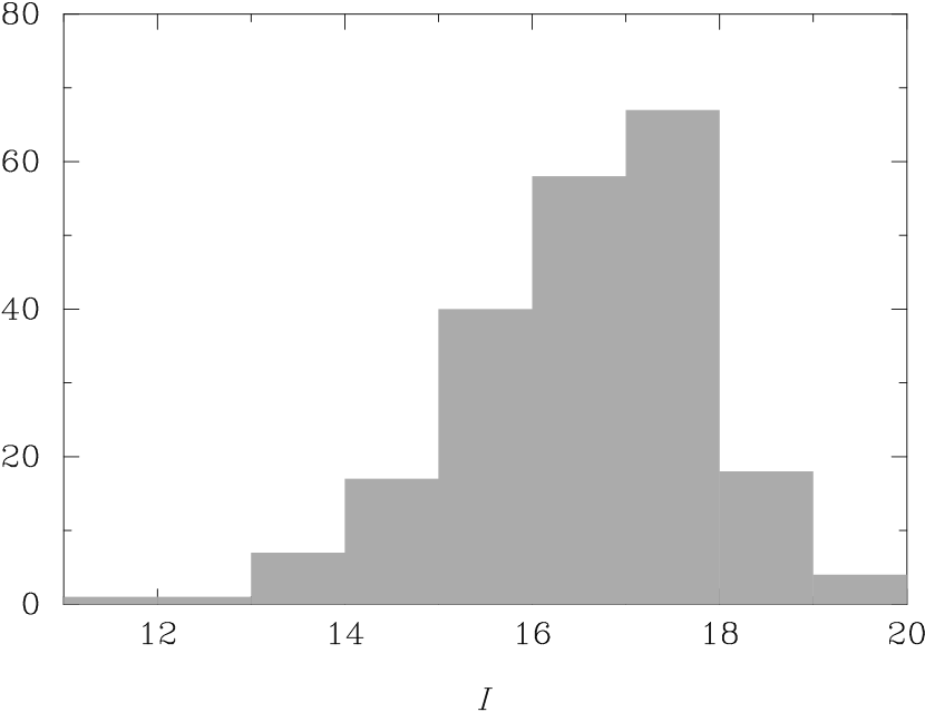
Figure 5: The first panel shows a histogram of $I$ magnitudes for 213 microlensing events observed by OGLE during 1997-1999. Of these, 26 have $I<15$, and 48 have $I<15.5$. The second panel shows the distribution of lensing rate with respect to angular Einstein radius, $d\Gamma/d\log\theta_{\rm E}$. The solid line shows the total rate distribution, the dashed line shows the distribution of events with $t_{\rm E}>50$ days, and the dotted line shows that for events with $t_{\rm E}>100$ days.

The next step is to determine the brightnesses and Einstein radii for typical events. Figure 5 illustrates the properties of bulge events. The first panel shows the distribution of peak $I$ magnitudes (or in cases where the peak was not observed, the brightest observed magnitude) for events observed by the OGLE collaboration during the 1997-1999 seasons. Assuming that sources with $K<14$ can be observed interferometrically, and assuming that $I-K=1.5$, we estimate that roughly 20% of events are bright enough to be followed up with interferometers. However, future surveys may go deeper than OGLE-II, returning a smaller fraction of bright events. Next, we turn to the distribution of Einstein radii. Since this has not been measured, we must estimate theoretically what the distribution will be.

The rate of microlensing events depends upon the properties of the lenses and source stars. We assume two types of stars, bulge stars and disk stars. For the disk stars, we use the mass function of Gould et al. (1997), namely $dN/dM\propto(M/M_{b})^{\alpha}$, with $M_{b}=0.59M_{\odot}$, and $\alpha=-0.56$ for $M_{\rm min}<M<M_{b}$, and $\alpha=-2.21$ for $M_{b}<M<M_{\rm max}$. We take $M_{\rm min}=0.1M_{\odot}$ and $M_{\rm max}=100M_{\odot}$. The disk density profile is taken to be $\rho(r_{l})=\rho_{0}e^{r_{l}/r_{d}}$, where $\rho_{0}=8~{}10^{7}M_{\odot}/{\rm kpc}^{3}$ is the local density, $r_{d}=3.5$ kpc is the disk scale length, and $r_{l}$ again is the distance of the lens from us towards the source, taken to be at the Galactic center. The velocity distribution of disk stars is taken to be a flat rotation curve $v_{c}=220$ km/s, along with velocity dispersion in each transverse direction of $\sigma_{d}=30$ km/s. For the bulge stars, we use the mass function of Zoccali et al. (2000), which has the same form as the disk MF but with $M_{b}=1M_{\odot}$, $\alpha=-1.33$ for $0.15M_{\odot}<M<M_{b}$, and $\alpha=-2$ for $M_{b}<M<100M_{\odot}$. The bulge density distribution we use is based on the barred model of Han & Gould (1995), with $\rho(r_{l})=\rho_{0}\exp[-\frac{w}{2}(r_{s}-r_{l})^{2}]$, with central density $\rho_{0}=2.07~{}10^{9}M_{\odot}/{\rm kpc}^{3}$, $w=(\cos i/x_{0})^{2}+(\sin i/y_{0})^{2}$ with scale lengths $x_{0}=1.58$ kpc, $y_{0}=0.62$ kpc and inclination $i=20^{\circ}$. Bulge stars are taken to have no net rotation and a velocity dispersion in each transverse direction of $\sigma_{b}=110$ km/s.

Lenses are drawn from both the disk and bulge populations. For simplicity, we assume that all sources lie at the galactic center, with the bulge velocity distribution. We neglect the motion of the local standard of rest relative to the flat rotation at $v_{c}$. The distribution of Einstein radii is given in the Appendix by Eqn. (A8) and Eqn. (A). Using the above parameter values, the resulting rate distribution is plotted in the second panel of Fig. 5. Clearly, a large fraction of events should have $\theta_{\rm E}$ accessible to instruments like the Keck Interferometer or VLTI.

As mentioned earlier, for very long timescale events ($t_{\rm E}>50$ days) the parallax may be measured with sufficiently high quality photometry, meaning that measurement of $\theta_{\rm E}$ gives the mass and distance. Estimating that $\sim 15\%$ of events are of sufficiently long duration, that $\sim 10\%$ are bright enough to be observed with VLTI or Keck, and that 1000 events are detected every year we expect to measure masses for about 15 microlensing events from the ground every year. This should be interesting for constraining the high end of the mass function.

However, VLTI and Keck can observe many more events than just those showing parallax, if there is justification to do so – for example, if such measurements could better constrain the lens properties. Let us wildly speculate about a massive campaign from VLTI to observe 100 events per year. The basic observable from such a campaign is the joint distribution of event timescales $t_{\rm E}$ and angular Einstein radii $\theta_{\rm E}$. An expression for $d\Gamma/d\theta_{\rm E}dt_{\rm E}$ is derived in the appendix in Eqn. (A10). The resulting rate distribution is plotted in Fig. (6).

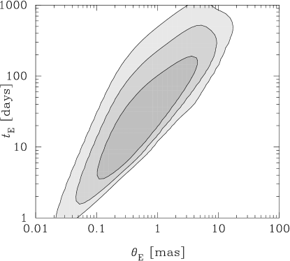
Figure 6: Contours of $d\Gamma/d\log\theta_{\rm E}d\log t_{\rm E}$, spaced by decades.

A massive survey can measure a noisy sample of this distribution. To estimate how well these measurements may be used to constrain the underlying lens properties, we use the Fisher matrix (Gould, 1995; Tegmark et al., 1997). For a likelihood distribution $L$ (here $d\Gamma/d\theta_{\rm E}dt_{\rm E}$) with parameters $\lambda_{i}$, the covariance matrix of the parameters estimated by sampling $L$ is given by

$$c_{ij}=({\bf b}^{-1}){ij}$$ (25)

where the matrix b has elements

$$b_{ij}=\left\langle\frac{\partial\log L}{\partial\lambda_{i}}\frac{\partial\log L}{\partial\lambda_{j}}\right\rangle$$ (26)

and the angular brackets denote integration over possible observables (here $\theta_{\rm E}$ and $t_{\rm E}$) weighted by $L$. We vary eight parameters: the bulge velocity dispersion $\sigma_{b}$, mass function parameters $\alpha_{1}$, $\alpha_{2}$ and $m_{p}$, and the same parameters for the disk lenses. Results are listed in Table 1. We find that the corresponding disk and bulge parameters are somewhat degenerate, as may be expected, but that large numbers of events can allow constraints to be placed on the bulge parameters. For example, with $N=400$ lenses the error on the slope of the high end of the bulge mass function becomes $\Delta\alpha_{2}=0.2$, and the error on $m_{p,b}$ becomes $0.18M_{\odot}$, sufficient to detect a break in the mass function and to localize the break position. The caveat to this statement is that we have made several simplifying approximations, for example not exploring degeneracies between the mass function parameters and the density profile parameters.

parameter	value	error ($N=1$)
$\sigma_{b}$	110 km/s	108 km/s
$m_{p,b}$	1 $M_{\odot}$	3.6 $M_{\odot}$
$\alpha_{1b}$	-1.33	7.9
$\alpha_{2b}$	-2	3.8
$\sigma_{d}$	30 km/s	466 km/s
$m_{p,d}$	0.59 $M_{\odot}$	4.0 $M_{\odot}$
$\alpha_{1d}$	-0.56	43.3
$\alpha_{2d}$	-2.21	9.3

Table 1: Errors on parameters from measuring $d\Gamma/d\theta_{\rm E}dt_{\rm E}$. The second column lists the adopted values for each parameter, and the third column lists the measurement errors estimated using the Fisher matrix. The errors values are to be multiplied by $N^{-1/2}$, where $N$ is the number of bright lens events observed by the interferometer.

5 Discussion

Interferometry is poised to revolutionize the study of microlensing events. Until now, microlensing has suffered the difficulty that masses of individual lenses cannot be measured, severely limiting the information able to be extracted from lensing surveys. The problem has been that the two quantities needed to measure mass and distance, the relative parallax $\pi_{\rm E}$ and the angular Einstein radius $\theta_{\rm E}$, are not regularly measured. The parallax may be measured for long duration events with high quality photometry, however measurement of $\theta_{\rm E}$ requires resolution on the order of a milliarcsecond, necessitating interferometers. The upcoming Space Interferometry Mission (SIM) should measure masses and distances for a large sample of lenses, answering the question of the microlenses’ nature. Well in advance of SIM, however, ground-based interferometers can also provide useful measurements of lensing events.

As mentioned earlier, microlensed sources are generally much fainter than the typical sources studied by optical interferometers, meaning that large apertures ($\sim 8$m) are required. Both the Keck Interferometer and the VLTI can measure visibility amplitude for microlensing events using their largest apertures, but only VLTI can measure closure phase using 3 large apertures; the Keck would be required to employ one of the 1.8 m outrigger telescopes which collect considerably fewer photons. The signal measured by interferometers is a function of the Einstein radius in units of the resolution, $\theta_{\rm E}B/\lambda$. Because of this, there is great advantage to go to shorter wavelengths. However, shorter wavelengths require the use of adaptive optics (AO) systems. Since AO makes the accurate calibration of visibility very difficult, but has a smaller impact on the calibration of closure phase, there are obvious advantages to using closure phase. For a numerical example, a microlensing event with $\theta_{\rm E}=0.5$ mas could be observed at 10 $\mu$m without AO, but $\theta_{\rm E}B/\lambda\sim 0.02$ giving a visibility signal of $V\approx 0.99$, which would be extremely challenging to distinguish from a point source. The same event observed at 2.2 $\mu$m using AO has $\theta_{\rm E}B/\lambda\sim 0.11$ giving a closure phase signal $\phi_{123}\approx 2.5^{\circ}$ which can already be measured.

Only a small fraction of events are expected to be bright enough ($K\lesssim 14$) to be observed interferometrically. However, certain fainter events may also be accessible to interferometers. If a bright ($K<13$) star falls within the isoplanatic angle, then phase referencing may be employed to extend the coherence time significantly. As noted earlier, for sites with small isoplanatic patches the probability of finding a suitable bright star is poor. Additionally, this technique is quite complex and as yet unproven, however in principle this could allow the study of microlensing events as faint as 20th magnitude, reaching the bright end of LMC events. Phase referencing must be employed to perform narrow angle astrometry; our results indicate that events for which phase referencing is possible may be more profitably studied with visibility or closure phase.

We expect that $\sim 15$ events every year will be bright enough ($K<14$) and have sufficiently long duration ($t_{\rm E}>50$ days) to permit the measurement of mass and distance. We have shown that a fairly large fraction of events accessible to ground-based interferometers should allow measurement of $\theta_{\rm E}$ with high signal to noise. We also investigated the prospects for a massive follow-up campaign by VLTI, and found that statistical information on the $\theta_{\rm E}$ distribution, even without individual mass measurements, can allow constraints to be placed on lens properties like their mass function.

Even if our estimates turn out to be overly optimistic, interferometers will still be able to elucidate the nature of claimed black hole candidates (e.g. Mao et al., 2002; Bennett et al., 2002). Agol et al. (2002) have suggested that current microlensing data indicate the presence of a significant population of intermediate mass black holes roaming the Galactic disk; interferometers will be able to confirm or reject this possibility.

In this paper, we have focused on ground-based interferometers, however our results apply also to space-based interferometers like the Space Interferometry Mission (SIM). SIM is primarily an astrometric instrument, however it can also measure fringe visibilities. Nominally, the target precision expected for SIM is 1% in $V^{2}$ (M. Shao 2002, priv. comm.). SIM’s baseline is 10m, and typical wavelengths are $\lambda\approx 0.6\mu$m, giving resolution of about 12 mas. Hence, SIM can determine $\theta_{\rm E}$ with SNR$>10$ from visibility alone, entirely independently of the astrometric determination, for events with $\theta_{\rm E}>0.44$ mas. From Figure 5 we see that this comprises a large fraction of the events. The visibility measurements come for free with the astrometric measurements, and should significantly increase the precision of SIM mass measurements, as long as effects such as crowding do not pose too great an obstacle. In addition to measuring $\theta_{\rm E}$, SIM also determines $\pi_{\rm E}$, the lens parallax, by measuring the time of the peak of the photometric lightcurve. Since the peak of the visibility signal coincides with the peak of the photometric signal, SIM visibility measurements could also be used to determine $\pi_{\rm E}$. However, since the variation in $1-V^{2}$ is so shallow near the peak this method may not prove to be as precise as ordinary photometric parallax measurement.

One of the most (potentially) exciting prospects is a topic we have not discussed in this paper, binary microlensing. For a binary lens system, complicated caustic structures can arise, leading in favorable cases to the production of 5 images of the source. For a spectacular example of this, see An et al. (2002). During caustic crossings, the magnification can get exceptionally large, e.g. factors of 30, making these events bright enough to observe with interferometers. The five images are currently unresolvable from each other, however VLTI and Keck offer the prospect of imaging the multi-image pattern. With a multi-aperture system (required for closure phase), one obtains several visibility measurements and one closure phase at the same time, possibly allowing the reconstruction of complex events such as caustic crossings.

Appendix A Appendix - Microlensing rate

The microlensing optical depth $\tau=\int n\sigma dl$ is given by

$$\tau=\int_{M_{\rm min}}^{M_{\rm max}}dM\frac{dN}{dM}\int_{0}^{r_{s}}dr_{l}~{}n(r_{l})\pi r_{l}^{2}\theta_{\rm E}^{2},$$ (A1)

where $dN/dM$ is the mass function of lenses, normalized by $\int(dN/dM)dM=1$, $n(r_{l})=\rho(r_{l})/\bar{M}$ is the number density of lenses, $\bar{M}=\int(dN/dM)MdM$ is the average mass and $\rho$ is the mass density of lenses. From Eqn. 1, we then have

$$\frac{d\tau}{d\theta_{\rm E}} = \int_{M_{\rm min}}^{M_{\rm max}}dM\frac{dN}{dM}\int_{0}^{r_{s}}dr_{l}~{}n(r_{l})\pi r_{l}^{2}\theta_{\rm E}^{2}\delta\left[\theta_{\rm E}-\left(\frac{4GM}{c^{2}}\frac{r_{s}-r_{l}}{r_{s}r_{l}}\right)^{1/2}\right]$$ (A2)

$$= \frac{\pi c^{2}}{2G}\theta_{\rm E}^{3}\int_{0}^{r_{s}}dr_{l}\frac{r_{s}r_{l}^{3}}{r_{s}-r_{l}}\frac{\rho(r_{l})}{\bar{M}}\frac{dN}{dM}[m(\theta_{\rm E},r_{l})]$$

where $m(\theta_{\rm E},r_{l})=(c^{2}/4G)\theta_{\rm E}^{2}r_{s}r_{l}/(r_{s}-r_{l})$.

The optical depth distribution describes the instantaneous properties of lensing events at any given time, but we are interested in the distribution of all events. This is described by the lensing rate $\Gamma=n\sigma v$. If the transverse velocity distribution of source stars is $f_{s}({\bm{v}}_{s})$, and that of the lenses is $f_{l}({\bm{v}}_{l})$, we can write the lensing rate as (Griest, 1991)

$$\Gamma=\int dM\frac{dN}{dM}\int_{0}^{r_{s}}dr_{l}2r_{l}\theta_{\rm E}n(r_{l})\bar{v}_{T}(r_{l})$$ (A3)

where

$$\bar{v}_{T}(r_{l})=\int d^{2}v_{l}d^{2}v_{s}f_{l}({\bm{v}}_{l})f_{s}({\bm{v}}_{s})|{\bm{v}}_{T}|$$ (A4)

$${\bm{v}}_{T}={\bm{v}}_{l}-(1-x){\bm{v}}_{o}-x{\bm{v}}_{s}.$$ (A5)

Here, ${\bm{v}}_{o}$ is the observer’s velocity transverse to the line of sight, and $x=r_{l}/r_{s}$. We assume all sources are bulge stars, with no net rotation and a velocity dispersion in each transverse direction of $\sigma_{b}$. Lenses are assumed to reside either in the bulge or in the disk, with the latter population possessing a flat rotation curve $v_{c}$, along with velocity dispersion in each transverse direction of $\sigma_{d}$. For bulge lenses, this gives

$$\bar{v}_{T}(r_{l})=\frac{1}{(1+x^{2})\sigma_{b}^{2}}\int v^{2}dv\exp\left(-\frac{v^{2}+(1-x)^{2}v_{c}^{2}}{2(1+x^{2})\sigma_{b}^{2}}\right)\frac{1}{2\pi}\int_{0}^{2\pi}\exp\left(-\frac{(1-x)v_{c}v}{(1+x^{2})\sigma_{b}^{2}}\cos\theta\right)d\theta.$$ (A6)

As usual, the angular integral gives a Bessel function, but note that it is a modified Bessel function due to the lack of an $i$ in the exponent. Thus we have

$$\bar{v}_{T}(r_{l}) = \frac{\exp\left[-\frac{(1-x)^{2}v_{c}^{2}}{2(1+x^{2})\sigma_{b}^{2}}\right]}{(1+x^{2})\sigma_{b}^{2}}\int v^{2}dv\exp\left(-\frac{v^{2}}{2(1+x^{2})\sigma_{b}^{2}}\right)I_{0}\left[\frac{(1-x)v_{c}v}{(1+x^{2})\sigma_{b}^{2}}\right]$$

$$= \sqrt{\frac{\pi}{2}}\frac{e^{-\frac{(1-x)^{2}v_{c}^{2}}{4(1+x^{2})\sigma_{b}^{2}}}}{\left(4(1+x^{2})\sigma_{b}^{2}\right)^{1/2}}\left[\left((1-x)^{2}v_{c}^{2}+2(1+x^{2})\sigma_{b}^{2}\right)I_{0}\left(\frac{(1-x)^{2}v_{c}^{2}}{4(1+x^{2})\sigma_{b}^{2}}\right)\right.$$

$$\left.\hskip 144.54pt+(1-x)^{2}v_{c}^{2}I_{1}\left(\frac{(1-x)^{2}v_{c}^{2}}{4(1+x^{2})\sigma_{b}^{2}}\right)\right]$$

For disk lenses, the expression is similar, with $(1-x)v_{c}\to xv_{c}$ and $(1+x^{2})\sigma_{b}^{2}\to\sigma_{d}^{2}+x^{2}\sigma_{b}^{2}$.

From Eqn. (A3), the distribution of rate with respect to angular Einstein radius is

$$\frac{d\Gamma}{d\theta_{\rm E}} = \int dM\frac{dN}{dM}\int_{0}^{r_{s}}dr_{l}2r_{l}\theta_{\rm E}n(r_{l})\bar{v}_{T}(r_{l})\delta\left[\theta_{\rm E}-\left(\frac{4GM}{c^{2}}\frac{r_{s}-r_{l}}{r_{s}r_{l}}\right)^{1/2}\right]$$ (A8)

$$= 4\int_{0}^{r_{s}}dr_{l}r_{l}n(r_{l})\bar{v}_{T}(r_{l})m(\theta_{\rm E},r_{l})\frac{dN}{dM}\left[m(\theta_{\rm E},r_{l})\right].$$

Lastly, we also want the joint distribution of rate with respect to $\theta_{\rm E}$ and $t_{\rm E}$. This is

$$\frac{d\Gamma}{d\theta_{\rm E}dt_{\rm E}}=4\int_{0}^{r_{s}}dr_{l}r_{l}n(r_{l})m(\theta_{\rm E},r_{l})\frac{dN}{dM}\left[m(\theta_{\rm E},r_{l})\right]\int d^{2}v_{l}d^{2}v_{s}f_{l}({\bm{v}}_{l})f_{s}({\bm{v}}_{s})v_{T}\delta\left(t_{\rm E}-\frac{r_{l}\theta_{\rm E}}{t_{\rm E}}\right).$$ (A9)

For bulge lenses, this is

$$\frac{d\Gamma}{d\theta_{\rm E}dt_{\rm E}} = 4\int_{0}^{r_{s}}dr_{l}n(r_{l})m(\theta_{\rm E},r_{l})\frac{dN}{dM}\left[m(\theta_{\rm E},r_{l})\right]\frac{r_{l}^{4}\theta_{\rm E}^{3}}{t_{\rm E}^{4}}$$ (A10)

$$\qquad\times\frac{\exp\left[-\frac{(r_{l}\theta_{\rm E}/t_{\rm E})^{2}+(1-x)^{2}v_{c}^{2}}{2(1+x^{2})\sigma_{b}^{2}}\right]}{(1+x^{2})\sigma_{b}^{2}}I_{0}\left[\frac{(1-x)v_{c}r_{l}\theta_{\rm E}/t_{\rm E}}{(1+x^{2})\sigma_{b}^{2}}\right].$$

For disk lenses, the expression is similar, with $(1-x)v_{c}\to xv_{c}$ and $(1+x^{2})\sigma_{b}^{2}\to\sigma_{d}^{2}+x^{2}\sigma_{b}^{2}$.

References

- Agol et al. (2002) Agol, E., Kamionkowski, M., Koopmans, L. V. E. & Blandford, R. D. 2002, submitted to ApJ, astro-ph/0203257
- Akeson, Swain & Colavita (2002) Akeson, R. L., Swain, M. R., Colavita, M. M., 2002, Proc. SPIE, 4006, 321-327.
- Alcock et al. (1997) Alcock, C. et al. 1997, ApJ, 479, 119
- Alcock et al. (2001) Alcock, C. et al. 2001, ApJ, 542, 281
- An et al. (2002) An, J. et al. 2002, ApJ, 572, 521
- Baldwin et al. (1996) Baldwin, J. E. et al. 1996, A&A, 306, L13-L16.
- Bennett et al. (2002) Bennett, D. P., et al. 2002, astro-ph/0109467
- Berger et al. (2001) Berger, J. P. et al. 2001, A&A376, L31-L34.
- Boden et al. (1998a) Boden, A. F., Shao, M. & Van Buren, D. 1998a, ApJ, 502, 538
- Boden et al. (1998b) Boden, A. F., et al. 1998b, ApJ, 504, L39
- Boden et al. (1999) Boden, A. F., et al., 1999, ASP Conf. Ser. 194: Working on the Fringe: Optical and IR Interferometry from Ground and Space, pp. 84+.
- Colavita (1999) Colavita, M. M. 1999, PASP, 111, 111
- Coude du Foresto et al. (2001) Coude du Foresto, V., et al. 2001, Comptes Rendus de l’Academie des Sciences IV - Phys. 2, 45-55.
- Delplancke et al. (2000) Delplancke, F. et al., 2000, Proc. SPIE, 4006, 365-376.
- Delplancke et al. (2001) Delplancke, F., Górski, K. M. & Richichi, A. 2001, A&A, 375, 701
- Glindemann et al. (2000) Glindemann, A., et al. 2000, Proc. SPIE Vol. 4006, p. 2-12, Interferometry in Optical Astronomy, Pierre J. Lena; Andreas Quirrenbach; Eds.
- Gould (2000) Gould, A. 2000, ApJ, 542, 785
- Gould (1995) Gould, A. 1995, ApJ, 440, 510
- Gould et al. (1997) Gould, A., Bahcall, J. N. & Flynn, C. 1997, ApJ, 482, 913
- Gould & Salim (1999) Gould, A. & Salim, S. 1999, ApJ, 524, 794
- Griest (1991) Griest, K. 1991, ApJ, 366, 412
- Guyon (2002) Guyon, O., 2002, A&A, 387, 366-378.
- Han & Gould (1995) Han, C. & Gould, A. 1995, ApJ, 447, 53
- Hummel et al. (1998) Hummel, C. A., et al. 1998, AJ, 116, 2536
- Jennison (1958) Jennison, R. C. 1958, MNRAS, 118, 276
- Lawson (2001) Lawson, P. R. 2001, “Principles of Long Baseline Interferometry”, http://sim.jpl.nasa.gov/library/coursenotes.html
- Mao et al. (2002) Mao, S., et al. 2002, MNRAS, 329, 349
- Paczyński (1986) Paczyński, B. 1986, ApJ, 304, 1
- Paczyński (1998) Paczyński, B. 1998, ApJ, 494, L23
- Segransan (2002) Segranan, D., 2002, SF2A-2002: Semaine de l’Astrophysique Francaise, meeting held in Paris, France, June 24-29, 2002, Eds.: F. Combes and D. Barret, EdP-Sciences (Editions de Physique), Conference Series.
- Shaklan & Roddier (1988) Shaklan, S., Roddier, F., 1988, Appl. Opt., 21, 2334.
- Shao & Colavita (1992a) Shao, M. & Colavita, M. M. 1992, ARA&A, 30, 457
- Shao & Colavita (1992b) Shao, M. & Colavita, M. M. 1992, A&A, 262, 353
- Shao et al. (2000) Shao, M., Boden, A. F., Colavita, M. M., Lane, B. F., Lawson, P. R. 2000; BAAS, 195, 87.14
- Tango & Twiss (1980) Tango, W. J., Twiss, R. Q., 1980, In: Progress in optics. Volume 17. (A81-13109 03-74) Amsterdam, North-Holland Publishing Co., p. 239-277
- Tegmark et al. (1997) Tegmark, M., Taylor, A. N. & Heavens, A. F. 1997, ApJ, 480, 22
- Thompson et al. (1986) Thompson, A. R., Moran, J. M. & Swenson, G. W. Jr. 1986, “Interferometry and Synthesis Imaging in Radio Astronomy”, New York: Wiley-Interscience
- Zoccali et al. (2000) Zoccali, M. et al. 2000, ApJ, 530, 418