SHEEP: THE SEARCH FOR THE HIGH ENERGY EXTRAGALACTIC POPULATION

Abstract

We present the SHEEP survey for serendipitously-detected hard X-ray sources in ASCA GIS images. In a survey area of $\sim 40$ deg², 69 sources were detected in the 5-10 keV band to a limiting flux of $\sim 10^{-13}$ erg cm^-2 s^-1. The number counts agree with those obtained by the similar BeppoSAX HELLAS survey, and both are in close agreement with ASCA and BeppoSAX 2-10 keV surveys. Spectral analysis of the SHEEP sample reveals that the 2-10 and 5-10 keV surveys do not sample the same populations, however, as we find considerably harder spectra, with an average $\Gamma\sim 1.0$ assuming no absorption. The implication is that the agreement in the number counts is coincidental, with the 5-10 keV surveys gaining approximately as many hard sources as they lose soft ones, when compared to the 2-10 keV surveys. This is hard to reconcile with standard AGN “population synthesis” models for the X-ray background, which posit the existence of a large population of absorbed sources. We find no evidence of the population hardening at faint fluxes, with the exception that the few very brightest objects are anomalously soft. 53 of the SHEEP sources have been covered by ROSAT in the pointed phase. Of these 32 were detected. An additional 3 were detected in the RASS. As expected the sources detected with ROSAT are systematically softer than those detected with ASCA alone, and of the sample as a whole. Although they represent a biased subsample, the ROSAT positions allow relatively secure catalog identifications to be made. We find associations with a wide variety of AGN and a few clusters and groups. At least two X-ray sources identified with high-z QSOs present very hard X-ray spectra indicative of absorption, despite the presence of broad optical lines. A possible explanation for this is that we are seeing relatively dust-free “warm absorbers” in high luminosity/redshift objects. Color analysis indeed indicates that many of the spectra are not consistent with a simple, absorbed power law. The spectra are likely to be complex, with an absorbed hard power law and scattered or “leaky” component in the soft X-rays. Many are also consistent with a reflection dominated spectrum. Our analysis defines a new, hard X-ray selected sample of objects - mostly active galactic nuclei - which is less prone to bias due to obscuration than previous optical or soft X-ray samples. They are therefore more representative of the population of AGN in the universe in general, and the SHEEP survey should produce bright examples of the sources that make up the hard X-ray background, the majority of which has recently been resolved by Chandra. This should help elucidate the nature of the new populations.

1 INTRODUCTION

ROSAT observations have shown that the diffuse X–ray background (XRB) in the soft X-ray band (0.5-2 keV) is made up of discrete sources, primarily standard, broad-line QSOs (Shanks et al. 1991; Hasinger et al. 1998; Schmidt et al. 1998). It is puzzling, however, that the X-ray spectra of AGN above $\sim 2$ keV, which typically show an intrinsic power law index of $\sim 1.9$ (Nandra & Pounds 1994), is so much steeper than the observed background in the same band, with $\Gamma\sim 1.4$ (Marshall et al. 1980). This “spectral paradox” has received much attention, and a consensus appears to be emerging as to its resolution. Setti & Woltjer (1989) suggested that the spectral paradox can be solved by hypothesizing that large numbers of AGN are heavily absorbed in the X-ray band, consistent with Seyfert unification schemes (Lawrence & Elvis 1982; Antonucci & Miller 1985). Comastri et al. (1995), and other authors (e.g. Madau, Ghisselini & Fabian 1994; Gilli et al. 1999, 2001) have shown that AGN spectra with a range of absorbing column densities can indeed be made to fit the XRB spectrum consistently with the number counts. Such models of the XRB are the most promising to date, and agree with many observables, including the range of spectra seen in nearby, bright AGN. They predict that the major contributors to the XRB are a large population of highly-absorbed AGN at moderate-high redshift. This population of objects has never been directly observed. This is perhaps not surprising, given that traditional UV-excess and soft X-ray surveys - which have detected most of the AGN we know of so far - are biased against strongly-absorbed objects.

The best method of uncovering obscured AGN is in the hard X-ray band, and a large population of such sources is implied. The ROSAT 0.5-2 keV number counts can be converted into 2-10 keV counts by extrapolating the ROSAT flux assuming the mean spectrum of the ROSAT sources of $\Gamma=2$. This exercise under-predicts the number counts observed by ASCA by a factor $\sim 2$ (Georgantopoulos et al. 1997; Cagnoni et al. 1998; Ueda et al. 1999a). This immediately implies the presence of a large population with flat or absorbed spectra. Optical spectroscopic identifications of ASCA sources have identified a few examples of obscured AGN at high redshift. For example, Boyle et al. (1998) have reported the discovery of an X-ray obscured quasar at z=0.67 and Georgantopoulos et al. (1999) have described the properties of an even more extreme z=2.35 quasar (see Akiyama, Ueda & Ohta 2002 for another example). Chandra has now also uncovered a few examples of type II QSOs (Norman et al. 2001; Stern et al. 2002). The inferred column densities for these sources are $>10^{23}$ cm^-2 which makes them extremely difficult to detect or identify in soft X-ray surveys and, if the absorbing material is dusty, heavily redenned and weak in the optical. There may be a vast population of such hidden beasts lurking in the hard X-ray sky.

A promising start towards uncovering this population has been made using the BeppoSAX HELLAS survey. Fiore et al. (1999) presented the first results of a survey in the 5-10 keV with the BeppoSAX MECS instrument. Their survey covered an area of 50 deg² and detected $\sim$150 sources above a limiting flux of about $5\times 10^{-14}$ erg cm^-2 s^-1. The updated HELLAS survey of Fiore et al. (2001) covers a larger area of 85 deg^-2, with 147 sources. The number count distribution, logN-logS, presents a Euclidean slope with $\gamma=1.56\pm 0.14$, in apparent agreement with the population synthesis models (Comastri et al. 2001). At the survey’s limiting flux $\sim 30$ per cent of the 5-10 keV XRB has been resolved. Catalog cross-correlations and the results of an optical ID program showed a high proportion of AGN, many of which are heavily obscured and some of which are at moderately high redshifts (Fiore et al. 1999; Fiore et al. 2001). This survey contains several examples of obscured AGN both because of its large area and of the very hard X-ray band employed. Preliminary results from XMM on the Lockman hole field (Hasinger et al. 2001) has extended the logN-logS a factor of twenty deeper (see also Baldi et al. 2001). It appears to present a Euclidean slope all the way down to the limiting XMM flux of $2.4\times 10^{-15}$. At this flux limit 60 per cent of the 5-10 keV XRB has been resolved.

New data from Chandra have now provided a breakthrough in our understanding of the XRB, but have also raised further questions. Mushotzky et al. (2000) presented observations of a deep Chandra-ACIS field. They detected a few tens of sources most of which have been spectroscopically followed up with the Keck telescope (Barger et al. 2001). Surprisingly there were no numerous examples of the long sought obscured “type II QSO” population (note we adopt the traditional definition of type I and type II objects based on their optical, rather than X-ray properties). Instead two other distinct populations appear. One is of bright early-type galaxies. These galaxies are “passive”, in that they present no clear sign of AGN activity in their optical spectra. The other population of X-ray sources is of hard sources with very faint or non-existent optical counterparts (even in deep Keck images, implying $B>28$ in some cases). This immediately highlights a problem with the Chandra population - that they are too faint for effective optical or X-ray followup. Deeper observations in the Chandra Deep Field South (CDFS), and in the Hubble Deep Field North (HDFN) respectively confirm the above findings (Tozzi et al. 2001; Brandt et al. 2001a) . For example, Brandt et al. (2001a) detect 12 sources in the area of the HDF (at a flux limit of $\sim 2\times 10^{-16}$ $\rm erg~{}cm^{-2}~{}s^{-1}$ in the 2-8 keV band) of which 4 are passive early-type galaxies while only 3 are broad-line AGN. The early, tentative suggestion is that the bulk of the X–ray background may arise from relatively low luminosity, low redshift AGN of uncertain character.

Further progress is possible by undertaking a large area hard X-ray survey, which can in principle reveal bright examples of the faint Chandra sources, to help understand their nature. HELLAS has already made some progress in this regard. Here we present a similar survey with the ASCA GIS instruments, called SHEEP (Search for the High Energy Extragalactic Population).

2 DATA ANALYSIS

The Gas Imaging Spectrometers (GIS; Tashiro et al. 1995) aboard the ASCA satellite (Tanaka, Inoue & Holt 1994) are ideal instruments for undertaking a wide angle hard X-ray survey. They have a relatively large field-of-view ($\sim 0.3$ deg²) and cover a broad energy range (0.7-10 keV) with good sensitivity, low background and moderate spatial resolution (HPD$\sim 3$ arcmin; Serlemitsos et al. 1995). A few dedicated survey projects were undertaken during the mission, but as ASCA was in operation for over 6 years mainly in pointed mode, it thereby accumulated serendipitous data on a large number of fields. We have used as a starting point for the SHEEP survey the “Tartarus” database of ASCA observations of AGN (Turner et al. 2002). This is ideal for our purposes, as most of the original ASCA targets are point-like, and many of them relatively weak. Fields with bright or extended targets are less useful, as they spread out over the GIS field of view, making it difficult to detect objects serendipitously.

2.1 Field Selection

We began with 464 ASCA observation sequences in version 1 of the Tartarus database. We rejected fields with a) exposure less than 30 ksec (combined GIS2+GIS3) b) Galactic latitude $|b|<20$ and c) targets brighter than 0.02 ct s^-1 in the 5-10 keV band. Bright targets can dominate the whole field due to the extended wings of the PSF, dramatically increasing the effective background. We also rejected a few fields for miscellaneous reasons, for example if the pointings were at extended sources (another was rejected due to contamination by a bright off-axis source). Finally, where multiple observations of the same target source existed, we chose the one with the highest exposure. This gave a total of 149 fields used in our survey. We restricted our analysis to the central 18 arcmin region of the GIS detectors and, as described below, excluded an area of 5 arcmin radius around the ASCA target. This results in a total area for the survey of 38.9 $\rm deg^{2}$.

2.2 Data reduction

Cleaned event files were taken from the Tartarus processing described in Turner et al. (2002). We extracted sky images in the 5-10 keV band for the GIS2 and GIS3 detectors from these using FTOOLS V5.0 and co-added them to produce a combined image. We then smoothed this with a gaussian of FWHM 1.8 arcmin and examined it visually for sources, marking the position of all candidates, regardless of whether they were close to the target position or not. We extracted counts from a cell of radius 5 pixels (75 arcsec). The area of the resultant detection cell was approximately $4$ arcmin². We determined the expected background in the detection cell using the “mkgisbgd” tool, which averages a large number of deep GIS pointings with sources removed. The predicted background in the cells was on average $\sim 17$ ct, but could be as low as $\sim 7$ ct. This means that a Gaussian approximation to the Poisson statistics could not be employed. We therefore determined the Poisson significance of each source based on the predicted and actual counts. We also performed spot checks on some images using a Mexican hat wavelet transform, and found our detection mechanism to be robust. After source detection, we discarded all objects with a position within 5 arcmin of the intended target of the observation. We chose this relatively large exclusion radius not only to exclude the original ASCA targets, but to account for possible extent in the targets and spurious sources representing the PSF wings (the ASCA PSF is highly azimuthally asymmetric; Serlemitsos et al. 1995).

3 THE SURVEY

3.1 Detected Sources

Table 1 shows the objects detected in our survey. We detected 69 sources with a significance above a Poisson probability threshold of $3\times 10^{-5}$ or approximately 4.5$\sigma$ for the equivalent Gaussian distribution. Considering our survey area and detection cell size this results in less than one source expected by chance. The table shows the (centroided) source position, the Poisson probability and the equivalent gaussian “sigma”. The count rate shown is the raw rate summed over the two GIS detectors in the 5-10 keV band. In order to convert these into a flux, we need to account for the size of the detection cell and the instrumental sensitivity at the particular off-axis angle of the source. We achieved this by extracting the spectrum of the source, and using the “ascaarf” task to determine the effective area for the extracted region. This was then compared to the on-axis effective area and the count rate corrected to represent an effective on-axis rate, also shown in the Table. Count rates were converted to fluxes assuming a spectrum of $\Gamma=1.6$, giving a conversion factor of $1.24\times 10^{-10}$ erg cm^-2 s^-1 per combined GIS ct s^-1. The assumed spectrum is in fact rather softer than our inferred mean spectrum ($\Gamma\sim 1.0$), but we adopt this value for the Table as it was also used by HELLAS (Fiore et al. 2001), and the ASCA 2-10 keV survey of Cagnoni et al. (1998) and Della Ceca et al. (1999), allowing an easier comparison. Adoption of the flatter slope makes a difference of 10 per cent in the derived flux, so this difference does not introduce a severe error, but we discuss the effects of the assumed slope on our results below. Our faintest source has a corrected count rate of $7\times 10^{-4}$ ct s^-1 corresponding to a flux of $9\times 10^{-14}$ erg cm^-2 s^-1 (5-10 keV) with our assumed spectrum.

3.2 Number Counts

Figure 1: (left panel) The area covered by our survey as a function of the flux limit. (right panel) The 5-10 keV SHEEP logN-logS (solid line) compared to the deepest point in the BeppoSAX HELLAS survey (open square; Fiore et al. 2001) and the ASCA 2-10 keV logN-logS (dashed line; Cagnoni et al. 1998) converted to the 5-10 keV band using $\Gamma=1.6$, The dash-dot line represents the XMM logN-logS derived by Baldi et al. (2001).

In Fig. 1 we plot the number count distribution, logN-logS, in the 5-10 keV band for our sample. To calculate this, it is first necessary to determine the detection threshold as a function of area for each image (left panel of Fig. 1). We did this by producing the exposure and effective area maps using the “ascaexpo” and “ascaeffmap” tasks. A background map was constructed using the “mkgisbgd” tool, and upper limits calculated assuming Poisson statistics. This was then converted into an effective flux limit using the effective area map. We show the resultant integral logN-logS distribution in the right panel of Fig. 1. A maximum likelihood fit gives $N(>S)=5(S/S_{0})^{-1.68^{+0.25}_{-0.25}}$ deg^-2, where $S_{0}=10^{-13}$ erg cm^-2 s^-1. We find excellent agreement with the logN-logS derived from the BeppoSAX HELLAS survey (Fiore et al. 2001), and the XMM number counts from Baldi et al. (2001), which reach fainter fluxes. We can also compare with the ASCA 2-10 keV logN-logS (Cagnoni al. 1998) converted to the 5-10 keV band again assuming a mean source spectrum of $\Gamma=1.6$. We see that the Cagnoni et al. logN-logS, $N(>S)\approx 10^{-21}S^{-1.67}$ deg^-2 (in the 5-10 keV band) provides a good fit to both the SHEEP and HELLAS data. At the faintest flux probed by our survey we resolve about 15% of the 5-10 keV XRB, using the HEAO-1 XRB normalization of Marshall et al. (1980). We note again here that in calculating the fluxes of the SHEEP sources, we have adopted $\Gamma=1.6$, softer than the inferred mean for our sample. Using the most extreme mean spectrum for our analysis of hardness ratios (see below) of $\Gamma=0.8$ would lead to a 10 per cent increase in all the fluxes, and therefore a $\sim 15$ per cent difference in logN-logS between SHEEP and the other surveys.

4 ROSAT observations and identifications

ROSAT observed the whole sky in the all-sky survey phase, and a very large fraction of the SHEEP objects in its pointed phase (see Table 2 for details). Any available ROSAT data are useful for our purposes, as they give both additional constraints on the colors/spectrum of the SHEEP sources, and also better positional accuracy for optical followup. We have cross-correlated the SHEEP catalog with several ROSAT catalogs, specifically the Rosat All Sky Survey (RASS) bright and faint-source catalogs, the WGACAT pointed catalog, and the ROSHRI HRI pointed image catalog. We found a total of 35 SHEEP sources associated with a ROSAT source within 2 arcmin ($\sim 2\sigma$ GIS position), 3 of which were in the RASS catalogs only. Some are detected in several catalogs and in some cases there are several ROSAT catalog objects listed within 2 arcmin of the ASCA position. In practice many of these may in fact be the same source, with multiple listings in the catalogs. In all such cases we have examined the ROSAT images (see Fig. 2) and determined whether there are indeed multiple ROSAT counterparts within the ASCA error box. We find no such case.

We have assessed the chance co-incidence of the associations between the detected ASCA and ROSAT sources by offseting the SHEEP positions by a few arc minutes, and repeating the cross-correlation. Performing 10 such simulations we find that the number of expected false coincidences are 0.8, 3.1 and 0.5 for the RASS, WGACAT and ROSHRI respectively. Clearly most of the RASS and HRI detected objects are secure, but there is some ($\sim 10$ per cent) probability that a given WGACAT source is not in fact associated with the SHEEP source.

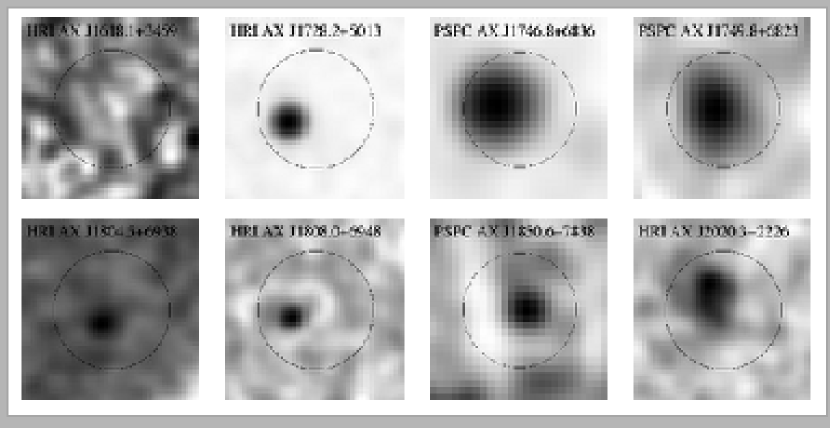
Figure 2: ROSAT “postage stamp” images for the SHEEP sources. The circles show a 2 arcmin radius centered on the ASCA position.

We have also independently analyzed the ROSAT data to determine upper limits for the SHEEP sources which were observed by ROSAT in the pointed phase, but not detected. In practice 53 SHEEP sources were within the 2-degree diameter FOV of a pointed ROSAT PSPC observation, and/or the ROSAT HRI FOV. Table 2 gives the details of these observations, in which we preferentially quote values from the HRI if possible, followed by pointed PSPC observations and finally RASS data where no pointed observation exists. We have extracted images for all of these, which are shown in Fig. 2, which also shows images for the 3 additional SHEEP listed in the RASS bright and faint-source catalogs. This independent analysis confirms the catalog cross-correlations listed above, revealing 32 ROSAT detections in pointed observations. In the 21 cases where no source was detected, we have derived upper limits to the ROSAT flux by extracting the counts from the entire 2 arcmin GIS error box, renormalizing to the 95 per cent PSF of the ROSAT PSPC or HRI, and calculating the 3$\sigma$ upper limit. The ROSAT non-detections cover a similar range of exposure time and off-axis angles to the detections, implying that the non-detections are not simply due to sensitivity issues. Apparently therefore a large fraction of the SHEEP sources ($\sim 40$ per cent) have extremely hard spectra rendering them undetectable by ROSAT. We discuss their spectral properties further below. A less likely alternative is that they are highly variable. The fraction of the SHEEP sources detected by ROSAT ($\sim 60$ per cent) is remarkably similar to the equivalent fraction of ROSAT-detected HELLAS sources (Vignali et al. 2001).

5 Catalog Identifications

The crucial remaining question for the X-ray background - which our survey can help to answer - is that of the nature of the sources which constitute the bulk of the XRB at hard X-ray energies. Our optical follow-up work is just beginning, but some indications can be gleaned without the use of telescope time by cross-correlating our X-ray catalog with existing data. This job is considerably easier for sources that have the more accurate ROSAT PSPC or (better still) HRI positions, which reduces the possibility of chance coincidences.

We have correlated the positions of the sources with ROSAT counterparts with the NASA/IPAC Extragalactic Database (NED). The ROSAT/NED associations are shown in Table 7.4. 19 SHEEP sources have NED counterparts within 1 arcmin (PSPC position) or 15 arcsec (HRI position). Although the latter is rather larger than the nominal positional error of the HRI, we allow for a large error in the HRI catalog positions as the sources may be far off axis, and the attitude solution is rather uncertain. Indeed we do find some very secure counterparts to HRI sources (e.g. bright QSOs or Sy 1) that are offset from the ROSAT positions by fairly large angles (see column 7 of Table 7.4). The dominant population is clearly AGN, but with many subclasses including classical QSOs, Seyfert 1s and more obscured Seyferts. Our highest redshift source is the QSO FBQS J125829.6+35284 at z=1.92. Unusually for a QSO this shows X-ray colors indicating a very hard spectrum (Table 1; see next section). Another example is CRSS J1429.7+4240. These are unusual because their optical spectral type indicates that there is an unobscured view of the nucleus but the X-ray colors are indicative of absorption. We shall return to this in the discussion.

Despite these few sources with hard spectra, we shall show in the next section that the ROSAT-detected sources are not a representative subsample of the SHEEP sources as a whole. Indeed, as might be expected, they are systematically softer. It is therefore extremely important to find and identify the optical counterparts of the X–ray sources that have not been detected by ROSAT, as these are the ones most likely to be fruitful in determining the origin of the hard X-ray background. We have therefore cross-correlated the entire SHEEP catalog with NED. Due to the large positional error of the GIS ($\sim 2$ arcmin), most of the resulting associations are probably random, the bulk being with anonymous radio (NVSS: Condon et al. 1998; FIRST: Becker, White & Helfand 1995 ) or 2MASS (Cutri et al. 2000) sources. These catalogs have rather high source densities and chance associations are likely. One such association that is likely to be real, however, is that of AX J1531.9+2420 with a radio loud quasar discovered in the FIRST survey, FBQS J153159.1+24204 at z=0.631 (White et al. 2000). For the others, it will be rather difficult to obtain unambiguous optical counterparts for the sources without improved hard X-ray positions.

6 Spectral properties

6.1 Hardness Ratios

Figure 3: Hardness ratios versus the 5-10 keV corrected count rate. HM denotes the 5-10 vs. 2-5 keV hardness ratio and HS the 5-10 versus 0.7-2 keV hardness ratio. Open squares are the 13 objects unobserved by ROSAT in the pointed phase. Filled circles were observed but not detected (21 objects). The 35 sources observed and detected by ROSAT are shown as the open triangles. As expected, the ROSAT-detected objects are significantly softer than those observed and not detected. Additionally, they are significantly softer than the mean of the sample as a whole, and form a biased subsample.

Figure 4: As in Fig. 3, but with the hardnesses binned according to 5-10 keV count rate large filled circles) along with the raw values (small open triangles). The binned values are unweighted, and the errors determined from the dispersion of the points. There is no trend for the hardness to change with flux, although the brightest four objects are clearly and significantly softer than the mean (Fig. 3). The mean hardnesses both correspond to a very flat spectrum, with $\Gamma\sim 0.8$, considerably harder than the spectra of objects found in 2-10 keV surveys (see text).

The SHEEP sources are selected in the 5-10 keV (“hard” = H) band, but we have also extracted the background subtracted count rates in the 2-5 keV (“medium”= M) band and the 0.7-2 keV (“soft”=S) band. These broad-band fluxes allow us to characterize the spectra of the sources in a crude manner. In Figs. 3 and 4 we plot the hard/medium ratio $HM=(H-M)/(H+M)$ and the hard/soft ratio $HS=(H-S)/(H+S)$ versus the hard band count rate. Note that in determining these ratios we have not corrected the counts for vignetting and the variable PSF. The energy dependence of these quantities is very weak (Serlemitsos et al. 1995) and correcting for these effects introduces an uncertainty larger than the correction. To the extent that these corrections change the hardness values, the effect is to make the corrected values slightly larger (i.e. harder).

Several things are noteworthy about Fig. 3. First, the hardness values can be used to determine the mean or typical effective spectral index for the objects. This is necessary for the conversion of count rates to flux, and also for comparing the typical spectrum of our objects to the X-ray background and those detected in other surveys. Determining the mean hardness of the sources is not straightforward, however, and the inferred spectrum depends on the method adopted. There are at least three ways of determining the mean HM and HS values: the unweighted average, the average weighted by the error bars and stacking. The last involves adding together all the individual H and M values (for example) and then computing HM from these summed fluxes. We prefer the first method (unweighted average) for determining the mean source spectrum as the last two can be strongly skewed by a small number of very bright sources. For example, the brightest source in our sample has a total number of M counts comparable to the sum of the entire remainder of the sample. The weighted and particularly the stacked HM value would therefore have little meaning, as it is largely representative of the spectrum of this single source, rather than the whole sample. The average hardness ratios of the full sample using all three methods are shown in Table 4. We have also calculated the average hardness for subsamples excluding the brightest source, and also the four brightest sources. Only the unweighted average gives consistent answers, showing how strongly the other methods can be biased by a very few bright sources.

Using the unweighted mean has the additional benefit of allowing us to estimate the error on the mean using the dispersion of the points which, at least in part, allows for some intrinsic dispersion in hardness values (see also Maccacaro et al. 1988). The unweighted mean HM value for our sample corresponds to a spectral index $\Gamma=0.7\pm 0.2$ assuming no absorption. The HS hardness gives a very similar spectrum, corresponding to $\Gamma=0.9\pm 0.2$. In practice the spectra may well be absorbed rather than showing this very flat photon index, but we note that the mean spectrum of our sources is significantly flatter than the integrated spectrum of the X-ray background in the 2-10 keV band, which has effective $\Gamma=1.4$ (e.g. Gendreau et al. 1995).

In Fig. 3, we have differentiated between sources which were detected by ROSAT either in the pointed phase or RASS, those which were observed in the pointed phase but not detected, and those which were not observed, except in the RASS. It is clear that the ROSAT detected sources, as might be expected, exhibit significantly softer spectra than both the ROSAT non-detections, and the sample as a whole. They are nonetheless quite hard, with mean HM equivalent to $\Gamma=1.4$ (Table 4). The ROSAT non-detections are extremely hard with equivalent $\Gamma\sim 0$ based on the HM color (Fig. 3 and Table 4). Many of our sources therefore clearly have spectra harder than that of the XRB. Fig. 4 shows the plot of the binned hardness ratio. This shows no tendency to harden with at faint fluxes, contrary to the findings of 2-10 keV surveys (Ueda et al. 1999b; Della Ceca et al. 1999; Giommi et al. 2000; Giacconi et al. 2001). It is clear from Fig. 3, however, that the very brightest sources are anomalously soft. For example, the brightest four objects in the sample have HM hardness corresponding to $\Gamma=2.1$, much softer than the mean, but fairly typical for unobscured AGN (e.g. Nandra & Pounds 1994). A total of 21 of the remaining SHEEP objects have a spectrum harder than this value at the 2$\sigma$ level.

There are disadvantages of using the straight average of the HM or HS values to determine the typical spectrum. One is that we give the same weight to data points that are very poorly determined as those that are very well determined. This should not matter if a sufficiently large number of points are averaged, but we note that a relatively large a fraction of SHEEP sources have hardnesses that are essentially undefined (i.e. the error on the HM or HS value spans the entire range of -1 to +1). To test whether these have a biasing effect, we have excluded from the averaging all such sources. There are 16 in total (Table 1). Excluding these does indeed result in a softer mean spectrum, as when the remaining 53 sources are averaged we find $\Gamma=1.3\pm 0.2$ from HM and a very similar value from HS (Table 4). This does not necessarily imply that the mean values from the entire sample are incorrect - it may simply be that the hardest sources have poorly defined hardness ratios. This is indeed expected, as very hard sources would be expected to have small and therefore uncertain M and/or S count rates. A related and potentially more serious problem is that of the Eddington bias. As we have performed the selection in the “H” band, sources around the flux threshold whose H counts randomly fluctuate in the positive direction will be deemed detections, while negative fluctuations will not. The M and S counts suffer no such (statistical) bias and therefore the weakest SHEEP sources should have HM and HS that are higher than the true values. We have tested this by considering only the SHEEP which have been detected at $>6\sigma$. The average HM and HS values of these most significant 34 sources again correspond to a softer spectrum of ($\Gamma\sim 1.3$). While this result may on the face of it seem to contradict the conclusion that the populations do not harden to faint fluxes, it does not. This is due to the large range of exposure times and off-axis angles for the SHEEP objects, such that flux and significance are not equivalent.

To attempt to mitigate both the effects described above, and to facilitate comparison with 2-10 keV surveys (see discussion) we have also calculate the hardness ratio denoted as “HR1” by, e.g., Ueda et al. (2001). This is defined in our notation as (H+M-S)/(H+M+S), i.e. the 2-10 keV vs 0.7-2 keV hardness. This should be much less affected by the Eddington bias as the effective area of the GIS is larger in the 2-5 keV band, and therefore the 2-10 keV counts will not typically be dominated by the 5-10 keV counts unless the spectrum is genuinely hard. We find HR1=$0.28\pm 0.05$ ($\Gamma=1.11\pm 0.11$) for the entire sample of 69 SHEEP. This does indeed imply a slightly softer spectrum than that derived from the HM or HS values (although it is consistent with the latter). Again considering only the 34 most significant sources in the sample we find $\Gamma=1.3\pm 0.1$ based on HR1, consistent at $90$ per cent confidence with the mean for the whole sample and therefore demonstrating the relative lack of bias in the HR1 ratio. This value is also completely consistent with those derived from the HM and HS hardnesses for the $>6\sigma$ subsample.

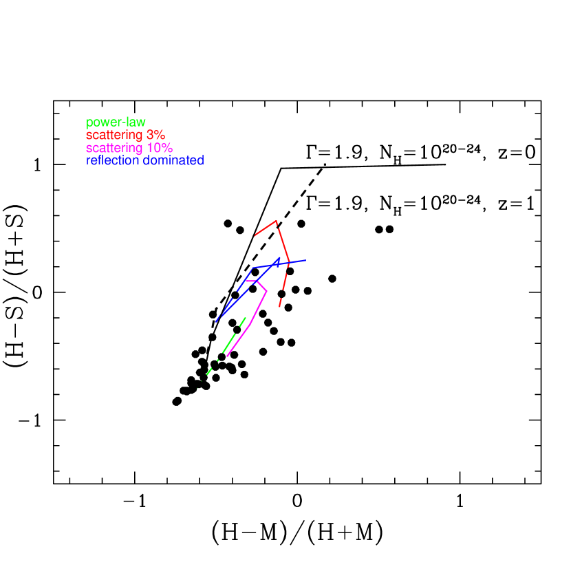
Figure 5: The X-ray color-color diagram. The S, M and H bands correspond to 0.7-2, 2-5 and 5-10 keV respectively. Sources with no detection in the 0.7-2 or 2-5 keV bands have been omitted for simplicity. The lines represent comparison spectra. The solid black line denotes the spectrum of an object at redshift z=0, a photon index of $\Gamma=1.9$ and a column density of $N_{H}=10^{20-24}$ $\rm cm^{-2}$ (left to right). The dashed line denotes the spectrum of an object at redshift z=1, a photon index of $\Gamma=1.9$ and a column density of $N_{H}=10^{20-24}$ $\rm cm^{-2}$ (left to right). The colors are generally no in good agreement with these simple, absorbed spectra. The green line represents a power-law spectrum with $\Gamma=1.0-1.9$ (right to left). The magenta line represents a partial coverer or scatterer model ($\Gamma=1.9$, column density $10^{24}\rm cm^{-2}$ scattering fraction $f=0.1$) from redshift z=0 to redshift z=2 (top to bottom). Another such model is shown in red, but this time with a covering fraction of $f=0.03$ Finally, the blue line represents the shift of a reflection dominated spectrum with an Fe line (see text for details) as a function of redshift (z=0 to z=2); the rightmost point corresponds to z=0. These “composite” models are able to reproduce the colors of a large fraction of the SHEEP sources.

In order to investigate the spectral properties of the individual sources in more detail, and in particular the role of absorption, we plot the X-ray color-color diagram in Fig. 5, in which we compare the HM and HS values with those predicted by various spectral models. It is evident from Fig. 5 that there is a wide range of spectral properties in our sample. Absorbed model spectra consisting of a power-law of $\Gamma=1.9$ (the typical AGN spectrum) and a column $N_{H}=10^{20-24}$ and z=0 are shown by the solid black line; at redshift z=1 (dashed line) the spectra are softer as the K-correction moves the absorption to energies outside the ASCA band. It is clear that, aside from the softest objects, which have unabsorbed power law spectrum and cluster at the bottom left of the diagram, colors of the SHEEP objects are not well represented by these simple, absorbed spectra. In particular a large fraction show a much harder HM color, for a given HS, than that for an absorbed power law. The green line represents a power-law spectrum with no absorption; the softest end of the line corresponds to $\Gamma=1.9$ while the hardest point is $\Gamma=1.0$. This is more consistent with the colors but many objects require extremely flat slopes ($\Gamma<1$). The physical origin of such flat power law slopes is unclear.

It is much more likely that the spectra of the SHEEP are complex, with both an absorbed hard component and softer emission. This “composite” model is typical of intermediate Seyfert galaxies (e.g. Seyfert 1.8 -1.9) in the local Universe (e.g. Turner et al. 1997). The red and magenta lines corresponds to scattering or partial covering models in which we assume that the hard X-ray emission is covered by an obscuring screen of $N_{H}=10^{24}$ cm^-2. Some fraction $f$ of the X-ray emission is either scattered into the line of sight or represents a “leaky” direct component. We evolve our models from redshift z=0 to z=2, and test two different covering fractions f=0.03 and f=0.1. We see that this model provides a good description for a large number of our sources and in particular is able to explain the sources which exhibit a very hard HM value, but relatively soft HS. Della Ceca et al. (1999) have reached similar conclusions regarding the composite nature of the spectra studying the spectral properties of a sample of ASCA sources detected in the softer 2-10 keV band. The BeppoSAX 2-10 keV and HELLAS surveys concur (Giommi et al. 2000; Vignali et al. 2001). The final model (blue line) shown in Fig 5 is a reflection dominated spectrum (e.g. Reynolds et al. 1994; Matt et al. 1996). The intrinsic illuminating spectrum has $\Gamma=1.9$ but the Compton reflection component has been enhanced by a factor of 100 compared to a slab subtending $2\pi$ solid angle at the X-ray source. An iron K$\alpha$ line at 6.4 keV of 1 keV equivalent width has also been included. Again this model is evolved from z=0 to z=2 and like the composite spectra, the reflection dominated model predicts harder HM values for a given HS. Indeed, the reflection dominated spectrum may be considered to be the extreme column density end of the “composite’ model. As is evident from Fig. 5, the predicted colors depend in detail on the column density, scattering (or covering) fraction and redshift. We can get only loose constraints on these from our color-color plot, but note that very high column densities ($\gg 10^{23}$ cm^-2) are required shift the HM colors significantly, particularly at high redshift.

Figure 6: HM hardness ratio versus redshift. The horizontal dashed lines show the HM values corresponding to two relevant values of the X-ray spectral index. A tentative correlation between hardness and redshift exists in the data, but with such a small number of objects we do not consider this to be a robust result.

Fig. 6 shows the HM hardness ratio versus redshift for the objects with catalogue identifications (Table 7.4). A tentative correlation can be seen between the source hardness and redshift, with both linear and Spearman rank correlations being significant at $>99$ per cent confidence. Clearly such a result would be of great interest, and similar results have been obtained in HELLAS (Comastri et al. 2001). We caution, however, that the very small number of objects in this plot means the true significance of our result is in some doubt. We therefore defer detailed discussion of the significance of such a correlation until redshifts are available for a larger number of the SHEEP sources, which will confirm or deny the result.

6.2 Spectral fitting

Figure 7: Spectral parameters for the 8 SHEEP sources with the highest signal-to-noise ratio in the 5-10 keV band (S/N$>10$). The photon index ($\Gamma$; upper panel) and absorbing column density ($N_{\rm H}$; lower panel) are plotted against the 5-10 keV flux in units of $10^{-12}$ erg cm^-2 s^-1. All parameters were derived from a spectral fit to the 1-10 keV GIS data with an absorbed power law model, assuming a minimum of Galactic $N_{\rm H}$. Only one spectrum shows evidence for significant absorption. This may only be revealed in the spectra of weaker objects, which requires data with higher signal-to-noise ratio.

A few of the SHEEP sources are bright enough to allow direct spectral fitting. Here we consider only the 8 sources in Table 1 which have gaussian S/N in the 5-10 keV band $>10\sigma$. We extracted the GIS2 and GIS3 spectra for these sources in the full band, and grouped them such that they had a minimum of 20 counts in each bin. Background was taken from adjacent source-free regions of the detector. We then fitted the spectra in the 1-10 keV band with model of a power law with a free, neutral absorber in the line-of-sight, in addition to fixed Galactic $N_{\rm H}$. The results are shown in Table 5.

The spectra are all well fit with this absorbed power law model with no evidence for any deviation from it. The mean spectral index is $\Gamma=1.94$ (unweighted) typical of the 2-10 keV spectra of bright, hard X-ray selected AGN (Nandra & Pounds 1994). This value is also similar to that of the soft X-ray background, and soft X-ray selected QSOs (e.g. Georgantopoulos et al. 1996; Blair et al. 2000). Although we find no general trend of hardening with decreasing flux in the sample, the spectral fitting does confirm the fact that the sources with the highest signal-to-noise ratio in our sample are softer than the whole. Only one of the sources with S/N$>10$ shows evidence for significant absorption in the line-of-sight, AX J2020.3-2226. Even this is relatively modest, at $2\times 10^{21}$ $\rm cm^{-2}$, with the upper limits for the other sources typically being less than this value. The softness of these very bright sources may explain why we typically find slightly softer spectra on average from the hardness ratio analysis when we split the sample according to signal-to-noise ratio. Although, as discussed above, there is not a one-to-one correspondence between flux and significance, these 8 sources with the with the highest signal-to-noise ratio are also the brightest ones in the SHEEP sample. While we have not found any general trend for hardening towards faint fluxes, it does therefore appear that the brightest few sources in the sample are softer than the average. Firm conclusions cannot be drawn about the origin of the XRB “spectral paradox” without good quality data on the weaker SHEEP sources, that are more typical of the sample and present colors consistent with the XRB spectrum.

7 DISCUSSION

We have performed an X-ray survey with the ASCA GIS in the 5-10 keV band in a $\sim 40$ deg² area to a flux level of $\sim 10^{-13}$ erg cm^-2 s^-1. 69 sources were detected, with a logN-logS distribution consistent with HELLAS, and 2-10 keV BeppoSAX and ASCA surveys. We resolve $\sim 15$% per cent of the hard X-ray background. Of the 69 sources, 35 have ROSAT counterparts and 19 of these have optical counterparts in catalogs. The classifications show that 11 of the ROSAT-detected sources are associated with type-1 AGN (i.e. Seyfert-1 and QSOs). We have shown, however, that the sources with ROSAT counterparts are preferentially softer than the remainder of the survey, and are therefore not an unbiased sample. A relatively large fraction (40%) of our sources were observed by ROSAT in the pointed phase, but not detected, and must therefore have extremely hard spectra.

The mean spectrum of the entire sample, as determined by the mean hardness ratio, depends on the method adopted and can be affected by statistical bias. However, we find that it is at least as hard as the X-ray background, and what should be the least biased estimate gives an equivalent $\Gamma=1.1\pm 0.1$. Unlike previous 2-10 keV surveys (e.g. Ueda et al. 1999b; Della Ceca et al. 1999; Giommi et al. 2000; Giacconi et al. 2001), we find no systematic hardening of the spectra to faint fluxes, although direct spectral fitting shows that the brightest few objects in our sample are anomalously soft. The spectra of the bulk of the individual sources are best described by a composite model, in which the power law is heavily absorbed, but some fraction of it either leaks through the absorber, or is scattered back into the line of sight. Some of the sources present very hard X-ray colors in the 2-10 keV band, much harder than the spectrum of the XRB. These may be very heavily absorbed, Compton thick sources such as NGC 6552 (Reynolds et al. 1994) and the Circinus galaxy (Matt et al. 1996). This type of object could be quite common, and be a major contributer to the peak of the XRB spectrum at $\sim 30$ keV.

7.1 Comparison with HELLAS and 2-10 keV surveys

A crucial question for our survey is that of whether it selects different objects than surveys in the 2-10 keV band. As the 2-10 keV observations are generally more sensitive, there would be no point in performing harder surveys such as ours if this were indeed the case. This issue was not addressed in the analysis of the HELLAS data. A related question is whether the 5-10 keV survey simply picks out hard (e.g. flat or absorbed) objects and misses soft ones, or whether 5-10 keV detection selects object in a less biased way. In the standard AGN synthesis picture where the objects are harder due to absorption we expect the latter to be the case. At the same equivalent flux limit, the 5-10 keV survey should pick up all of the unabsorbed objects, but it should also find absorbed objects that are missed in the softer surveys. This holds in part because the intrinsic spectral index of AGN is approximately $\Gamma=2.0$, and therefore equal intrinsic flux is emitted per unit energy. If the only modifier is absorption, then at the same flux limit the 5-10 keV survey should pick up all objects in the 2-10 keV surveys, and in addition all objects missed by the 2-10 keV surveys because their flux is depressed by absorption in the 2-5 keV band.

These issues are partially resolved by our analysis, although our data are somewhat contradictory. The fact that we (and HELLAS) find a very similar logN-logS function to the 2-10 keV surveys suggests that we are sampling the same populations. Two effects indicate that this is not the case, however. First, the hardness ratio analysis clearly indicates that the SHEEP sources have significantly harder spectra than those obtained in 2-10 keV surveys. As we have discussed above, the mean hardness ratios is rather difficult to calculate in a robust manner, and is subject to statistical bias, but we can compare our preferred value of $\Gamma=1.1\pm 0.1$ with that from 2-10 keV surveys. Both Della-Ceca et al. (1999) and Ueda et al. (1999) have presented mean values for 2-10 keV index derived from direct spectral fitting of stacked spectra. The former find $\Gamma=1.74\pm 0.07$, taking the weighted average of their “bright and “faint” subsamples, and the latter $\Gamma=1.49\pm 0.10$ from a 2-10 keV sample which was flux-selected to ignore the brightest sources. The “faint” subsample of Della Ceca et al. (1999) is marginally consistent with our preferred spectrum, with $\Gamma=1.36\pm 0.14$

Our analysis has highlighted the difficulty in determining the average spectral properties of sources detected in different ways in different surveys. To provide what is perhaps the fairest possible comparison, we have computed the HR1 hardness ratio for a subsample of the ASCA sources of Ueda et al. (2001). We considered only serendipitous sources (i.e. not the targets) and truncated their sample at a detection level of 4.5$\sigma$ (i.e. our detection threshold) in the 2-10 keV band, which resulted in a total of 601 sources. The mean, unweighted HR1 value of this sample is HR1=$-0.02\pm 0.01$, corresponding to $\Gamma=1.75\pm 0.02$. The corresponding HR1 for our sample is stated in Table 4 and corresponds to $\Gamma=1.11\pm 0.11$. These surveys were performed with the same instrument, and the hardness ratios were calculated in the same band and by the same method. The only substantive difference should therefore be the selection band (2-10 keV in the Ueda et al. subsample vs. 5-10 keV for SHEEP). We further note that the Eddington bias should artificially harden the value from the 2-10 keV survey (because the sources were selected in that band) but not the mean SHEEP spectrum. Thus we can firmly conclude that, based on the spectral form, our 5-10 keV survey selects a different and much harder population than 2-10 keV surveys.

Although the logN-logS functions are similar in the 2-10 keV and 5-10 keV bands, a few more objects can be accomodated in the 5-10 keV counts, particularly given the uncertainty in spectral shape and therefore the conversion of counts to flux. To put this on a more quantitative footing, we have taken the maximum difference in the logN-logS normalization comparing our and Cagnoni et al.’s 2-10 keV survey of 15 per cent. Could this additional 15 per cent of objects harden our average spectrum sufficiently to cause the difference between our survey and the 2-10 keV samples? We have tested this by excluding the hardest 9 sources (i.e. 15%) based on their HR1 value) from the SHEEP sample and recomputing the hardness ratio. We find a mean hardness for these 60 sources corresponding to $\Gamma=1.33\pm 0.07$, still considerably flatter than the 2-10 keV value. Similar results are found when excluding objects based on their HM and HS hardnesses. We can therefore further conclude that the 5-10 keV survey does not simply pick up a few additional hard objects compared to the 2-10 keV surveys, but rather samples a different population.

Additional supporting evidence for this conclusion comes from the fact that we find no trend for the source population to harden at faint fluxes, which is found in the 2-10 keV surveys. HELLAS similarly fails to find such a correlation (Fiore et al. 2001), and we also note that the Chandra survey of Moretti et al. (2002) reveals no correlation between hardness and 2-10 keV flux, although such a correlation is observed with the flux in the softer 0.5-2 keV band (Giacconi et al. 2001; Moretti et al. 2002). While there is some evidence that the brightest objects in our survey are softer than the mean, it appears that the 5-10 keV selection methods digs into the faint, hard populations which make up the X-ray background much more quickly than the 2-10 keV surveys. Thus, despite the good agreement between the number counts, we cannot be sampling the same populations as the 2-10 keV surveys. Presumably this is also true of HELLAS, although no mean spectrum has been given for these sources. We are then led to the conclusion that the agreement between the 2-10 keV and 5-10 keV number counts is largely coincidental, with our 5-10 keV survey picking up many additional hard objects, but almost exactly compensating for this in terms of numbers by losing softer ones.

The fact that the number counts from the 5-10 and 2-10 keV surveys agree so well, but that the populations are clearly different spectrally is troubling for the population synthesis models (e.g. Madau, Ghisselini & Fabian 1994; Comastri et al. 1995, 2001; Gilli et al. 1999, 2001). The problem is that these models generally assume an intrinsic spectrum for AGN of the form $\Gamma=1.9$, typical of local AGN, or even flatter. The intrinsic flux of such a power law per unit energy is larger in the 5-10 keV band than in the 2-5 keV band or for that matter the 2-10 keV band. Furthermore, absorption is invoked for a very large fraction of these sources which further depresses the 2-5 and 2-10 flux relative to the 5-10 keV flux. For example 75 per cent of sources in the model of Gilli et al. (1999) have $N_{\rm H}>10^{23}$ cm^-2. At z=0, this column density suppresses the 2-10 keV flux by a factor $\sim 2$, while the 5-10 keV flux only changes by $\sim 15$ per cent. These numbers are almost identical for a more typical AGN synthesis source with $N_{\rm H}=10^{24}$ cm^-2 at z=1.5. Thus, if the populations synthesis models are correct, and the absorbed populations have the same luminosity function and evolutionary properties as the unabsorbed ones, we expect much higher number counts (perhaps by a factor $\sim 2$) in the 5-10 keV logN-logS than for the converted 2-10 keV. Such a conclusion is grossly incompatible with our data (Fig. 1), and those from HELLAS. We note, however, that Comastri et al. (2001) have claimed consistency of both the 5-10 keV and 2-10 keV number counts with the synthesis models. This may in part be due to the fact that the proportion of absorbed sources in the synthesis models depends on the flux limit. Specifically, a higher proportion of absorbed objects is expected at fainter fluxes. In this scenario, the apparent agreement in number counts means that at the flux limits probed by SHEEP and HELLAS, the number of heavily obscured sources must be very small. It is very hard to see how this can be the case given the strong difference in spectra we find between the 5-10 and 2-10 keV populations.

An alternative possibility is that there is a large population of very soft sources (unobscured and with $\Gamma>2.0$ ) which are missed in the 5-10 keV surveys and picked up at 2-10 keV. This is not postulated typically in the synthesis models, where the obscured populations dominate and where “soft excesses”, if present, never affect the spectra above 2 keV. We await further detailed modelling of the number counts to address these issues, but note that there have been some tentative suggestions that much of the X-ray background may be produced at low redshift ($z<1$; Tozzi et al. 2001; Rosati et al. 2002), in agreement with our finding that the luminosity function and/or evolution of the absorbed populations is likely to differ from that of standard QSOs.

7.2 The nature of the X-ray background sources

Chandra deep surveys have resolved most of the X-ray background into discrete sources (Mushotzky et al. 2000; Giacconi et al. 2001; Brandt et al. 2001b). The astrophysical nature of these sources remains mysterious, however. Many of them are extremely faint in the optical (Mushotzky et al. 2000; Barger et al. 2001; Alexander et al. 2001) making spectroscopic identification impossible. What is required to make further progress, then, is to find bright, nearby examples of these objects that can be detected and studied in more detail. To do this requires surveys with much larger area than those possible currently with Chandra. The SHEEP survey, like HELLAS, with its large area and hard X-ray selection criterion, provides such a sample. Indeed it is very clear from the failure of ROSAT to detect a large fraction of our sources (which are nonetheless very bright in the hard X-ray band), that there are a large number of hard and probably obscured sources. While these are likely AGN, how their astrophysics is related to the more familiar classes of Seyfert 1s, Seyfert 2s and QSOs in the local and soft X-ray universe remains an open question. Optical identification and detailed X-ray spectroscopy of our sample can resolve this issue.

One key question is whether our sources present hard spectra due to a large amount of intrinsic absorption or whether they are intrinsically hard. The population synthesis models predict the former, but it is possible that the sources which make up the hard X-ray background have flat spectra for other reasons, such as the radiation mechanism. For example, photon-starved Comptonization or bremsstrahlung emission from an ADAF would produce a spectrum similar to that of the X-ray background. A pure reflection spectrum, e.g. in the case of a Compton-thick Seyfert galaxy could produce an even flatter spectrum (Reynolds et al. 1994; Matt et al. 1996, 2000). We find no clear answer to this in our hardness ratio analysis, but the most likely situation is that the X-ray spectra are composite, with an absorbed, hard power law and soft emission that may be either scattered nuclear light, or a separate thermal component (see also Della Ceca et al. 1999; Giommi et al. 2000; Vignali et al. 2001). Followup observations of the HELLAS and SHEEP sources with XMM will determine this unambiguously.

One early indication from HELLAS was that there may be a population of “red quasars” (Webster et al. 1995), with hard and possibly absorbed X-ray spectra (Fiore et al. 1999; Vignali et al. 2000). Complete optical followup of the SHEEP sample will confirm this, but here we highlight another potentially interesting class, of hard QSOs (see also Comastri et al. 2001). Our cross-correlation with the NED catalog shows two sources which are classified optically as QSOs, but whose hardness ratios indicate extremely hard spectra that correspond to $\Gamma<1.0$ if they are unabsorbed. We do not have complete optical spectra or spectral energy distributions of these sources, so these may also be red quasars and absorbed in the optical. The QSO classification, however, implies that we are seeing the nuclear broad lines directly. Again these objects may simply have intrinsically hard spectra, but to flatten a more typical QSO spectrum of $\Gamma\sim 1.9$ to the hard value observed requires a column density $\gg 10^{23}$ $\rm cm^{-2}$. The dust associated with such gas would likely obliterate the optical/UV emission, including the broad lines, causing the source to appear as a type II quasar. That the broad lines are in fact observed implies that the line of sight is not particularly dusty. One possibility is that the gas-to-dust ratio in these objects differs substantially from Galactic values (Maiolino et al. 2001). Another is that we are seeing hot and /or photoionized gas - or “warm absorbers” (Halpern 1984) - at high redshift. Such a gas component is commonly observed in low redshift Seyferts (e.g. Nandra & Pounds 1994; Reynolds 1997; George et al. 1998). The low redshift analogue of these QSOs is the famous Seyfert galaxy NGC 4151, which shows strong UV emission and broad optical/UV emission lines, but which is heavily absorbed in the X-ray band. The most obvious explanation for this is that there is dust-free gas near the nucleus, and this interpretation is supported by the fact that the X-ray column NGC 4151 is apparently mildly ionized (Yaqoob, Warwick & Pounds 1989; Weaver et al. 1994).

7.3 A complete, hard X-ray selected sample

Our survey has defined a new, hard X-ray selected sample of AGN. Along with the HELLAS AGN, these will be the first complete samples since the HEAO-1 survey (Piccinotti et al. 1982). Many of the objects in the Piccinotti sample are the most heavily observed AGN and their detailed study has revealed much of what we know about nuclear activity in galaxies. Those sources were almost exclusively nearby Seyferts, however, and our survey has already revealed a large number higher-redshift and higher-luminosity AGN. Follow-up observations of these hard X-ray bright objects could revise our opinions of the central regions of AGN. If, as is suggested by the Chandra data, the majority of AGN have been missed by optical surveys, much of what we think we know about their properties could be misleading. With hard X-ray selection we avoid the biases against obscuration inherent in most other methods of selection, and if we can follow up these observations with high quality data in other wavebands, our opinions about AGN phenomenology could change dramatically.

7.4 Future work

Optical followup of our sources is already in progress, with an imaging program and some spectroscopy, particularly for the northern sources. A significant problem, however, is that the GIS positions are not alone sufficient to identify unambiguously the optical counterpart. ROSAT PSPC positions are better and HRI positions the best available, but as we have shown, the ROSAT detected sources represent a biased subsample, and these sources probably do not represent the population providing the bulk of the energy density of the X-ray background at 30 keV. What is really required is to obtain Chandra and/or XMM observations of our sources, which will give us the optical counterparts without ambiguity. Such observations have the added advantage that they will allow us to determine the X-ray extent and spectra of the source populations, providing a crucial piece in the puzzle of how the bulk of the extragalactic background light at hard X-ray energies is produced.

Table 1: The SHEEP Sample

AX	RA	DEC	S/N	Raw	Rate	hm	hs	Seq.	Exp
(1)	(2)	(3)	(4)	(5)	(6)	(7)	(8)	(9)	(10)
J$0026.3+1050$	00 26 19.0	$+10$ 50 40	6.2	$3.0\pm 0.8$	$10.4\pm 2.6$	$-0.59^{+0.11}_{-0.23}$	$-0.54^{+0.12}_{-0.25}$	74011000	86.9
J$0043.7+0054$	00 43 47.0	$+00$ 54 36	6.6	$3.6\pm 0.9$	$11.8\pm 2.9$	$-0.18^{+0.18}_{-0.35}$	$-0.24^{+0.16}_{-0.32}$	75020000	72.5
J$0044.0+0102$	00 44 03.7	$+01$ 02 27	7.4	$3.8\pm 0.9$	$26.2\pm 6.1$	$-0.52^{+0.10}_{-0.21}$	$-0.35^{+0.14}_{-0.28}$	75020000	72.5
J$0058.7+3019$	00 58 43.0	$+30$ 19 45	4.9	$2.4\pm 0.7$	$21.4\pm 6.6$	$0.52^{+0.48}_{-1.52}$	$1.00^{+-0.00}_{-2.00}$	74000000	79.1
J$0133.7-4303$	01 33 47.1	$-43$ 03 23	4.8	$2.2\pm 0.6$	$7.0\pm 2.1$	$-0.58^{+0.15}_{-0.30}$	$-0.67^{+0.11}_{-0.24}$	75074000	102.2
J$0140.1+0628$	01 40 08.1	$+06$ 28 06	8.3	$3.2\pm 0.6$	$11.3\pm 2.1$	$-0.43^{+0.11}_{-0.22}$	$0.54^{+0.46}_{-1.27}$	75042000	145.8
J$0144.9-0345$	01 44 54.2	$-03$ 45 19	5.9	$3.2\pm 0.8$	$21.5\pm 5.8$	$-0.60^{+0.11}_{-0.22}$	$-0.58^{+0.11}_{-0.23}$	75090000	73.1
J$0146.2-0354$	01 46 15.0	$-03$ 54 53	4.8	$2.5\pm 0.8$	$28.0\pm 8.8$	$0.17^{+0.83}_{-1.17}$	$0.34^{+0.66}_{-1.34}$	75090000	73.1
J$0207.7+3511$	02 07 44.3	$+35$ 11 14	6.6	$3.4\pm 0.8$	$23.5\pm 5.8$	$0.57^{+0.43}_{-1.46}$	$0.49^{+0.51}_{-1.49}$	75077000	77.1
J$0242.8-2326$	02 42 51.8	$-23$ 26 03	6.7	$3.6\pm 0.9$	$17.7\pm 4.3$	$-0.40^{+0.13}_{-0.27}$	$-0.59^{+0.10}_{-0.20}$	73005000	76.0
J$0335.2-1505$	03 35 16.7	$-15$ 05 55	6.7	$3.3\pm 0.8$	$19.2\pm 4.7$	$-0.63^{+0.09}_{-0.19}$	$-0.49^{+0.12}_{-0.25}$	74009000	82.5
J$0335.6-3609$	03 35 40.4	$-36$ 09 18	5.1	$2.5\pm 0.8$	$24.0\pm 7.3$	$0.70^{+0.30}_{-1.70}$	$0.24^{+0.76}_{-1.24}$	72007010	75.3
J$0336.9-3616$	03 36 58.3	$-36$ 16 11	8.0	$3.9\pm 0.9$	$35.7\pm 8.0$	$-0.65^{+0.09}_{-0.19}$	$-0.69^{+0.08}_{-0.17}$	72007010	75.3
J$0401.4+0038$	04 01 25.6	$+00$ 38 49	5.1	$3.1\pm 0.9$	$9.0\pm 2.7$	$-0.38^{+0.19}_{-0.38}$	$-0.02^{+0.30}_{-0.57}$	73016000	64.8
J$0440.0-4534$	04 40 02.9	$-45$ 34 59	8.5	$4.1\pm 0.8$	$17.3\pm 3.5$	$-0.26^{+0.14}_{-0.28}$	$0.16^{+0.22}_{-0.42}$	75050000	91.6
J$0443.3-2820$	04 43 21.5	$-28$ 20 53	32.0	$18.6\pm 1.8$	$92.6\pm 9.1$	$-0.57^{+0.04}_{-0.08}$	$-0.72^{+0.03}_{-0.05}$	75086000	62.3
J$0642.9+6751$	06 42 57.8	$+67$ 51 45	7.1	$2.8\pm 0.6$	$25.5\pm 5.6$	$-0.34^{+0.14}_{-0.28}$	$-0.56^{+0.10}_{-0.20}$	74003000	120.1
J$0836.2+5538$	08 36 13.9	$+55$ 38 48	6.3	$3.3\pm 0.8$	$13.9\pm 3.5$	$0.22^{+0.78}_{-1.22}$	$0.11^{+0.28}_{-0.52}$	74036000	79.9
J$0836.6+5529$	08 36 36.2	$+55$ 29 42	4.9	$2.3\pm 0.7$	$25.0\pm 7.8$	$0.06^{+0.94}_{-1.06}$	$0.01^{+0.99}_{-1.01}$	74036000	79.9
J$0843.0+5014$	08 43 04.5	$+50$ 14 29	4.8	$2.9\pm 0.9$	$11.8\pm 3.7$	$0.56^{+0.44}_{-1.56}$	$0.26^{+0.74}_{-1.26}$	75067000	63.2
J$0844.8+5004$	08 44 50.1	$+50$ 04 37	5.0	$2.7\pm 0.9$	$57.4\pm 18.0$	$0.19^{+0.81}_{-1.19}$	$0.87^{+0.13}_{-1.87}$	75067000	63.2
J$1035.1+3938$	10 35 10.1	$+39$ 38 09	5.0	$3.2\pm 1.0$	$12.5\pm 3.8$	$-0.09^{+0.26}_{-0.52}$	$-0.01^{+0.28}_{-0.55}$	72020000	56.0
J$1040.3+2045$	10 40 23.4	$+20$ 45 47	12.7	$8.0\pm 1.3$	$39.5\pm 6.5$	$-0.50^{+0.07}_{-0.14}$	$-0.58^{+0.06}_{-0.12}$	73040010	59.1
J$1107.0-1150$	11 07 00.2	$-11$ 50 45	4.8	$2.5\pm 0.8$	$24.6\pm 7.9$	$0.49^{+0.51}_{-1.49}$	$1.00^{+0.00}_{-2.00}$	75012000	69.9
J$1115.3+4043$	11 15 20.3	$+40$ 43 03	18.9	$10.0\pm 1.2$	$46.7\pm 5.8$	$-0.64^{+0.04}_{-0.09}$	$-0.76^{+0.03}_{-0.06}$	74035000	78.0
J$1115.4+5308$	11 15 24.1	$+53$ 08 07	5.9	$3.0\pm 0.8$	$53.3\pm 14.6$	$0.63^{+0.37}_{-1.63}$	$0.51^{+0.49}_{-1.51}$	74098000	70.7
J$1153.7+4619$	11 53 47.6	$+46$ 19 55	6.2	$3.1\pm 0.8$	$21.5\pm 5.5$	$-0.57^{+0.11}_{-0.22}$	$-0.57^{+0.11}_{-0.22}$	75056000	81.1
J$1218.6+0546$	12 18 40.1	$+05$ 46 17	5.6	$2.5\pm 0.6$	$9.3\pm 2.4$	$-0.46^{+0.15}_{-0.30}$	$-0.57^{+0.12}_{-0.24}$	74085000	115.4
J$1218.9+2957$	12 18 55.7	$+29$ 57 26	8.2	$4.6\pm 1.0$	$26.8\pm 5.7$	$-0.52^{+0.09}_{-0.19}$	$-0.17^{+0.15}_{-0.30}$	71046000	72.0
J$1219.4+0643$	12 19 28.7	$+06$ 43 42	9.4	$6.4\pm 1.4$	$31.1\pm 6.6$	$-0.65^{+0.07}_{-0.15}$	$-0.76^{+0.05}_{-0.11}$	74074000	45.6
J$1220.2+0641$	12 20 16.2	$+06$ 41 44	10.9	$7.2\pm 1.4$	$54.6\pm 10.8$	$-0.56^{+0.09}_{-0.17}$	$-0.73^{+0.05}_{-0.11}$	74074000	45.6
J$1228.4+1300$	12 28 26.2	$+13$ 00 22	4.9	$3.5\pm 1.1$	$12.1\pm 3.9$	$-0.68^{+0.10}_{-0.22}$	$-0.78^{+0.08}_{-0.16}$	74051000	46.0
J$1230.8+1433$	12 30 51.9	$+14$ 33 23	5.0	$2.5\pm 0.8$	$34.8\pm 10.8$	$-0.68^{+0.12}_{-0.24}$	$-0.77^{+0.09}_{-0.18}$	75031000	69.4
J$1231.5+1422$	12 31 33.5	$+14$ 22 50	5.5	$3.1\pm 0.9$	$8.2\pm 2.3$	$-0.33^{+0.19}_{-0.38}$	$-0.64^{+0.10}_{-0.21}$	75031000	69.4
J$1241.3+3501$	12 41 21.7	$+35$ 01 01	8.6	$4.7\pm 1.0$	$14.7\pm 3.0$	$-0.37^{+0.12}_{-0.24}$	$-0.29^{+0.13}_{-0.27}$	75081000	73.3
J$1243.8+1305$	12 43 50.0	$+13$ 05 17	5.9	$2.8\pm 0.8$	$28.3\pm 7.8$	$0.21^{+0.79}_{-1.21}$	$0.51^{+0.49}_{-1.86}$	75045010	75.9
J$1257.6+3525$	12 57 40.1	$+35$ 25 34	4.8	$2.6\pm 0.8$	$16.2\pm 4.9$	$-0.03^{+0.32}_{-0.62}$	$-0.40^{+0.19}_{-0.39}$	75078000	74.2
J$1258.4+3528$	12 58 29.6	$+35$ 28 16	5.8	$2.9\pm 0.8$	$27.3\pm 7.6$	$-0.21^{+0.21}_{-0.42}$	$-0.17^{+0.23}_{-0.44}$	75078000	74.2
J$1325.8-3920$	13 25 50.0	$-39$ 20 40	4.7	$1.6\pm 0.5$	$12.7\pm 3.7$	$-0.42^{+0.15}_{-0.30}$	$-0.58^{+0.11}_{-0.23}$	75002000	152.9
J$1354.0+3346$	13 54 01.0	$+33$ 46 27	6.2	$3.3\pm 0.9$	$46.5\pm 12.0$	$0.50^{+0.45}_{-1.50}$	$0.49^{+0.51}_{-1.49}$	75068000	73.3
J$1354.1+3341$	13 54 11.6	$+33$ 41 03	6.7	$3.4\pm 0.9$	$27.4\pm 6.8$	$-0.47^{+0.13}_{-0.27}$	$-0.51^{+0.13}_{-0.26}$	75068000	73.3
J$1405.4+2223$	14 05 26.9	$+22$ 23 27	7.1	$3.8\pm 0.9$	$21.3\pm 5.2$	$-0.50^{+0.12}_{-0.24}$	$-0.67^{+0.08}_{-0.17}$	72021000	65.7
J$1406.1+2233$	14 06 08.3	$+22$ 33 02	5.3	$2.9\pm 0.9$	$17.4\pm 5.2$	$-0.01^{+0.31}_{-0.60}$	$0.02^{+0.33}_{-0.62}$	72021000	65.7
J$1406.2+2228$	14 06 13.6	$+22$ 28 22	4.8	$2.7\pm 0.8$	$10.2\pm 3.2$	$0.03^{+0.97}_{-1.03}$	$0.87^{+0.13}_{-1.87}$	72021000	65.7
J$1425.2+2303$	14 25 13.7	$+23$ 03 19	4.9	$3.4\pm 1.1$	$18.2\pm 5.8$	$0.17^{+0.83}_{-1.17}$	$0.68^{+0.32}_{-1.68}$	73078000	49.5
J$1426.8+2619$	14 26 52.1	$+26$ 19 35	6.6	$3.0\pm 0.8$	$23.7\pm 5.9$	$-0.70^{+0.08}_{-0.16}$	$-0.77^{+0.06}_{-0.12}$	74073000	83.4
J$1426.9+2334$	14 26 54.3	$+23$ 34 58	4.8	$2.2\pm 0.7$	$41.1\pm 12.9$	$0.02^{+0.98}_{-1.02}$	$0.54^{+0.46}_{-1.54}$	76060000	82.8
J$1428.1+2337$	14 28 08.2	$+23$ 37 40	5.9	$2.7\pm 0.7$	$37.8\pm 10.3$	$-0.62^{+0.09}_{-0.90}$	$-0.72^{+0.07}_{-0.15}$	76060000	82.8
J$1429.7+4240$	14 29 45.0	$+42$ 40 41	6.6	$4.1\pm 1.1$	$33.6\pm 8.9$	$-0.27^{+0.19}_{-0.38}$	$0.02^{+0.27}_{-0.52}$	71044000	51.9
J$1500.1+3325$	15 00 09.2	$+33$ 25 06	5.2	$2.7\pm 0.8$	$58.3\pm 17.1$	$0.29^{+0.71}_{-1.29}$	$1.00^{+0.00}_{-2.00}$	75082000	75.0
J$1511.7+0758$	15 11 43.6	$+07$ 58 54	5.4	$2.8\pm 0.8$	$11.9\pm 3.3$	$-0.01^{+0.22}_{-0.43}$	$-0.39^{+0.15}_{-0.30}$	71004000	85.8
J$1511.7+5702$	15 11 47.9	$+57$ 02 42	5.6	$2.5\pm 0.7$	$17.8\pm 4.8$	$0.55^{+0.45}_{-1.55}$	$0.66^{+0.34}_{-1.66}$	73080000	98.5
J$1512.0+5708$	15 12 04.4	$+57$ 08 05	5.2	$2.2\pm 0.6$	$21.7\pm 6.3$	$-0.04^{+0.33}_{-0.64}$	$0.17^{+0.83}_{-1.17}$	73080000	98.5
J$1531.8+2414$	15 31 51.1	$+24$ 14 43	8.5	$3.5\pm 0.7$	$21.5\pm 4.1$	$-0.40^{+0.11}_{-0.22}$	$-0.61^{+0.07}_{-0.15}$	75055000	130.7
J$1531.9+2420$	15 31 56.5	$+24$ 20 22	11.4	$4.4\pm 0.7$	$38.9\pm 6.2$	$-0.60^{+0.07}_{-0.13}$	$-0.63^{+0.06}_{-0.13}$	75055000	130.7
J$1532.3+2401$	15 32 19.1	$+24$ 01 13	6.3	$2.6\pm 0.6$	$12.2\pm 2.9$	$-0.40^{+0.14}_{-0.29}$	$-0.24^{+0.17}_{-0.35}$	75055000	130.7
J$1532.5+2415$	15 32 33.1	$+24$ 15 13	8.6	$3.4\pm 0.6$	$20.7\pm 4.0$	$-0.35^{+0.12}_{-0.24}$	$0.49^{+0.51}_{-1.22}$	75055000	130.7
J$1545.2+4855$	15 45 13.6	$+48$ 55 06	4.8	$2.2\pm 0.7$	$25.8\pm 8.0$	$0.71^{+0.29}_{-1.71}$	$0.64^{+0.36}_{-1.64}$	75059000	83.7
J$1617.0+3506$	16 17 05.9	$+35$ 06 38	5.8	$2.3\pm 0.6$	$20.7\pm 5.4$	$-0.05^{+0.27}_{-0.52}$	$-0.12^{+0.25}_{-0.48}$	75000000	110.3
J$1617.2+3454$	16 17 15.5	$+34$ 54 36	5.1	$2.2\pm 0.6$	$13.0\pm 3.7$	$-0.74^{+0.09}_{-0.19}$	$-0.85^{+0.06}_{-0.11}$	75000000	110.3
J$1618.1+3459$	16 18 10.7	$+34$ 59 46	5.1	$2.3\pm 0.6$	$11.7\pm 3.3$	$-0.21^{+0.24}_{-0.47}$	$-0.46^{+0.16}_{-0.33}$	75000000	110.3
J$1728.2+5013$	17 28 13.9	$+50$ 13 28	57.6	$28.3\pm 2.0$	$191.3\pm 13.2$	$-0.75^{+0.02}_{-0.03}$	$-0.86^{+0.01}_{-0.02}$	73022000	79.5
J$1746.8+6836$	17 46 52.8	$+68$ 36 17	23.8	$12.7\pm 1.5$	$88.7\pm 10.1$	$-0.61^{+0.04}_{-0.09}$	$-0.72^{+0.03}_{-0.06}$	74033000	69.8
J$1749.8+6823$	17 49 50.1	$+68$ 23 19	9.5	$5.0\pm 1.0$	$47.1\pm 9.4$	$-0.59^{+0.09}_{-0.17}$	$-0.45^{+0.11}_{-0.22}$	74033000	69.8
J$1804.5+6938$	18 04 30.7	$+69$ 38 01	5.0	$2.2\pm 0.7$	$22.2\pm 6.5$	$-0.39^{+0.17}_{-0.34}$	$-0.49^{+0.14}_{-0.29}$	74086000	94.8
J$1808.0+6948$	18 08 05.9	$+69$ 48 21	7.1	$3.2\pm 0.7$	$20.1\pm 4.6$	$-0.57^{+0.09}_{-0.19}$	$-0.61^{+0.09}_{-0.17}$	74086000	94.8
J$1850.6-7838$	18 50 38.7	$-78$ 38 31	8.8	$3.1\pm 0.6$	$19.9\pm 3.7$	$-0.51^{+0.09}_{-0.19}$	$-0.56^{+0.08}_{-0.17}$	75008000	153.9
J$2002.7-3300$	20 02 47.1	$-33$ 00 15	5.2	$2.8\pm 0.8$	$11.1\pm 3.2$	$-0.14^{+0.24}_{-0.47}$	$-0.30^{+0.19}_{-0.39}$	73001000	75.2
J$2020.3-2226$	20 20 19.6	$-22$ 26 48	20.8	$8.1\pm 0.9$	$100.6\pm 11.4$	$-0.65^{+0.04}_{-0.08}$	$-0.71^{+0.03}_{-0.07}$	73075000	118.1

Note. — Col.(1): SHEEP object Col.(2): ASCA RA (2000) Col.(3): ASCA DEC (2000) Col.(4): Equivalent “sigma” (see text) Col.(5): Total GIS2+GIS3 counts in the 5-10 keV band divided by total exposure (GIS2+GIS3) in units of $10^{-4}$ ct s^-1 and $1\sigma$ uncertainty. Col.(6): Hard-band (5-10 keV) count rate and error corrected to on-axis value for a single GIS detector in units of $10^{-4}$ ct s^-1. These should be multipled by $1.24\times 10^{-10}$ to convert to flux in units of erg cm^-2 s^-1 for a $\Gamma=1.6$ spectrum. Col.(7): Hardness, defined as $(H-M/H+M)$ where $M$ is the medium energy (2-5 keV) rate. Col.(8): Hardness, defined as $(H-S/H+S)$ where $S$ is the soft (0.7-2 keV) rate. Col.(9): Sequence number in which this source was detected Col.(10): Total GIS+GIS3 exposure time for sequence (ks)

Table 2: ROSAT observations of SHEEP sources

AX	Seq	Exp	Theta	RX	Offset	Rate	$N_{\rm H}$(Gal)	Flux
(1)	(2)	(3)	(4)	(5)	(6)	(7)	(8)	(9)
J0026.3+1050	ROSHRI	30.0	9.2	J$002619.1+105021$	0.31	0.0053 $\pm$ 0.0006	6.0	1.63
J0043.7+0054	rp700377n00	10.7	39.2	$\cdots$	$\cdots$	$<0.01$	2.3	$<3.1$
J0044.0+0102	WGACAT	10.7	33.9	J$004401.4+010258$	0.77	0.0095 $\pm$ 0.0019	2.4	1.0
J0058.7+3019	rh701308n00	14.9	13.0	$\cdots$	$\cdots$	$<0.0060$	5.9	$<5.85$
J0133.7-4303	ROSHRI	2.4	8.2	J$013346.6-430417$	0.90	0.0097 $\pm$ 0.0025	1.8	3.06
J0140.1+0628	ROSHRI	4.3	8.0	J$014002.5+062732$	1.51	0.0035 $\pm$ 0.0013	4.1	1.14
J0207.7+3511	WGACAT	14.0	16.1	J$020744.1+351142$	0.47	0.0025 $\pm$ 0.0006	6.3	0.3
J0242.8-2326	ROSHRI	20.5	6.5	J$024252.3-232633$	0.51	0.0142 $\pm$ 0.0009	2.0	4.40
J0335.6-3609	rp700921a01	7.7	22.6	$\cdots$	$\cdots$	$<0.0125$	1.4	$<3.5$
J0336.9-3616	ROSHRI	6.2	16.7	J$033653.9-361617$	0.89	0.0099 $\pm$ 0.0023	1.4	3.1
J0401.4+0038	WGACAT	7.8	26.9	J$040125.9+003935$	0.77	0.0061 $\pm$ 0.0013	13.0	0.73
J0440.0-4534	rh702888n00	4.4	4.6	$\cdots$	$\cdots$	$<0.0012$	2.0	$<1.1$
J0443.3-2820	RASSBSC	0.1	$\cdots$	J$044320.8-282039$	0.28	0.15 $\pm$ 0.04	2.4	15.9
J0642.9+6751	WGACAT	5.3	7.5	J$064246.2+675222$	1.27	$0.0046\pm 0.001$	5.5	0.55
J0836.2+5538	rh703892n00	16.7	10.0	$\cdots$	$\cdots$	$<0.0062$	4.1	$<5.8$
J0836.6+5529	rh703892n00	16.7	13.3	$\cdots$	$\cdots$	$<0.0071$	4.1	$<6.8$
J0843.0+5014	WGACAT	8.7	4.0	J$084315.3+501415$	1.74	0.0032 $\pm$ 0.0007	3.1	0.35
J0844.8+5004	rp700318n00	8.7	14.0	$\cdots$	$\cdots$	$<0.0094$	3.0	$<3.0$
J1035.1+3938	rh701982n00	1.6	4.5	$\cdots$	$\cdots$	$<0.0016$	1.5	$<1.50$
J1040.3+2045	RASSFSC	0.36	$\cdots$	J$104027.5+204555$	1.02	0.10 $\pm$ 0.02	2.0	10.2
J1115.3+4043	ROSHRI	28.9	10.6	J$111521.2+404327$	0.42	0.0404 $\pm$ 0.0013	1.9	12.6
J1153.7+4619	WGACAT	4.4	7.8	J$115345.6+462022$	0.56	0.0107$\pm$ 0.0017	2.0	1.12
J1218.6+0546	rh701307a01	18.5	12.4	$\cdots$	$\cdots$	$<0.0055$	1.5	$<5.0$
J1218.9+2957	WGACAT	3.1	11.7	J$121854.8+295835$	1.16	0.0039 $\pm$ 0.0014	1.7	0.44
J1219.4+0643	ROSHRI	3.8	6.1	J$121930.8+064339$	0.48	0.0580 $\pm$ 0.0040	1.6	18.2
J1220.2+0641	ROSHRI	4.0	14.4	J$122018.3+064123$	0.59	0.0482 $\pm$ 0.0042	1.6	15.0
J1228.4+1300	rh701657n00	5.9	8.8	$\cdots$	$\cdots$	$<0.0011$	2.6	$<1.06$
J1230.8+1433	ROSHRI	4.4	16.5	J$123052.4+143305$	0.32	0.0145 $\pm$ 0.0029	2.5	4.8
J1231.5+1422	rh601003n00	4.4	4.1	$\cdots$	$\cdots$	$<0.0099$	2.5	$<9.6$
J1241.3+3501	ROSHRI	46.3	6.0	J$124123.9+350014$	0.92	0.0011 $\pm$ 0.0003	1.4	0.31
J1243.8+1305	rh701007a01	6.1	17.4	$\cdots$	$\cdots$	$<0.0075$	2.3	$<7.0$
J1257.6+3525	WGACAT	4.0	7.7	J$125745.4+352542$	1.08	0.0035 $\pm$ 0.0012	1.2	0.32
J1258.4+3528	WGACAT	17.2	9.	J$125829.4+352840$	0.40	0.0252 $\pm$ 0.0023	1.2	2.28
J1354.1+3341	RASSFSC	0.4	$\cdots$	J$135407.8+334039$	0.85	0.0298 $\pm$ 0.0107	1.2	2.64
J1405.4+2223	ROSHRI	1.6	10.4	J$140528.2+222321$	0.35	0.0172 $\pm$ 0.0037	2.1	5.4
J1406.1+2233	rh703968n00	1.7	11.3	$\cdots$	$\cdots$	$<0.00195$	2.1	$<1.90$
J1406.2+2228	rh703968n00	1.7	4.2	$\cdots$	$\cdots$	$<0.00177$	2.1	$<1.71$
J1425.2+2303	rh701899n00	5.7	9.0	$\cdots$	$\cdots$	$<0.0092$	2.7	$<12.4$
J1426.8+2619	WGACAT	6.7	16.3	J142652.5+261922	0.24	0.033 $\pm$ 0.0027	1.7	3.24
J1426.9+2334	WGACAT	3.0	10.0	J$142656.1+233651$	1.93	0.0045 $\pm$ 0.00015	2.7	0.49
J1428.1+2337	WGACAT	3.1	18.3	J$142807.4+233725$	0.30	0.0560 $\pm$ 0.0048	2.8	6.11
J1429.7+4240	WGACAT	9.5	13.7	J$142944.7+424106$	0.42	0.0149 $\pm$ 0.0016	1.4	1.41
J1512.0+5708	rp600190n00	18.1	53.6	$\cdots$	$\cdots$	$<0.0053$	1.5	$<1.43$
J1532.3+2401	rp701411n00	23.0	52.0	$\cdots$	$\cdots$	$<0.0061$	4.1	$<2.1$
J1532.5+2415	rp701411n00	23.0	49.7	$\cdots$	$\cdots$	$<0.0040$	4.1	$<1.40$
J1545.2+4855	rp700809n00	5.5	13.0	$\cdots$	$\cdots$	$<0.0013$	1.6	$<0.38$
J1617.0+3506	rh800164n00	33.4	7.9	$\cdots$	$\cdots$	$<0.0041$	1.4	$<3.7$
J1617.2+3454	ROSHRI	33.4	7.0	J$161720.5+345404$	1.12	0.0047 $\pm$ 0.0005	1.4	1.46
J1618.1+3459	rh800164n00	33.4	3.8	$\cdots$	$\cdots$	$<0.0038$	1.4	$<3.7$
J1728.2+5013	ROSHRI	1.6	1.4	J$172819.1+501309$	0.90	0.6068 $\pm$ 0.0192	2.7	437.0
J1746.8+6836	WGACAT	24.7	10.6	J$174658.2+683632$	0.56	0.2790 $\pm$ 0.0039	4.4	32.7
J1749.8+6823	WGACAT	24.7	19.8	J$174949.0+682321$	0.12	0.0094 $\pm$ 0.0008	4.5	1.1
J1804.5+6938	ROSHRI	18.2	16.9	J$180434.4+693734$	0.55	0.0065 $\pm$ 0.0013	4.5	2.1
J1808.0+6948	ROSHRI	18.2	8.0	J$180813.9+694806$	0.73	0.0036 $\pm$ 0.0006	4.8	1.17
J1850.6-7838	WGACAT	2.2	10.6	J$185028.8-783814$	0.56	0.0057 $\pm$ 0.0019	9.2	0.69
J2020.3-2226	ROSHRI	6.4	6.7	J$202021.5-222554$	1.00	0.0057 $\pm$ 0.0011	6.1	1.85

Note. — Col.(1): SHEEP object; Col.(2): ROSAT sequence or catalog; Col.(3): ROSAT exposure (ks); Col.(4): Off-axis angle (arcmin); Col.(5): ROSAT ID; Col.(6): Offset from ASCA position (arcmin); Col.(7): PSPC or HRI count rate in the 0.1-2 keV band (ct s^-1); Col.(8): Galactic $N_{\rm H}$ ($10^{21}$ cm^-2); Col(9): ROSAT flux in the 0.1-2.0 keV band in units of $10^{-13}$ erg cm^-2 s^-1;

Table 3: Catalog and literature IDs

AX	NED	RA	DEC	Class	$z$	Offset	Rad	IR	Ref
(1)	(2)	(3)	(4)	(5)	(6)	(7)	(8)	(9)	(10)
J$0242.8-2326$	FHC93 0240-2339A	02 42 51.9	$-23$ 26 34	QSO	0.68	0.1	N	N	2
J$0336.9-3616$	FCSS J033654.0-361606	03 36 54.0	$-36$ 16 07	QSO	1.54	0.2	Y	N	3
J$0443.3-2820$	HE0441-2826	04 43 20.7	-28 20 52	QSO	0.155	0.2	N	N	4
J$0642.9+6751$	NRRFJ064241.3+675257	06 42 41.3	$+67$ 52 57	G/Cl	$\cdots$	0.7	N	N	5
J$1115.3+4043$	2MASXi J1115208+40432	11 15 20.8	$+40$ 43 26	Sy1	0.076	0.1	N	Y	6
J$1218.9+2957$	1SAX J1218.9+2958	12 18 52.5	+29 59 01	Sy1.9	0.176	0.7	N	N	7
J$1219.4+0643$	MS 1217.0+0700	12 19 31.0	$+06$ 43 35	Sy1	0.08	0.1	N	N	3
J$1230.8+1433$	VPC0774	12 30 52.7	$+14$ 33 03	G	$\cdots$	0.1	N	N	8
J$1258.4+3528$	FBQS J125829.6+352843	12 58 29.6	$+35$ 28 43	QSO	1.92	0.1	Y	N	9
J$1405.4+2223$	RIXOS F274-008	14 05 28.3	$+22$ 23 33	Sy1	0.156	0.2	N	N	10
J$1426.8+2619$	Zw 1424.6+2632	14 26 50.0	$+26$ 18 34	Cl	$\cdots$	1.0	N	N	11
J$1428.1+2337$	KUG 1425+238	14 28 07.7	$+23$ 37 23	G	$\cdots$	0.1	N	N	12
J$1429.7+4240$	CRSS J1429.7+4240	14 29 45.1	$+42$ 40 54	QSO	1.67	0.2	N	Y	13
J$1617.2+3454$	NGC6107	16 17 20.1	$+34$ 54 05	G/Group?	0.03	0.1	Y	N	14
J$1728.2+5013$	1 Zw 187	17 28 13.9	$+50$ 13 10	QSO	0.055	0.1	Y	N	15
J$1746.8+6836$	VII Zw742	17 47 00.1	$+68$ 36 37	G/Pair	0.063	0.2	N	Y	3
J$1749.8+6823$	KUG 1750+683A	17 49 50.6	$+68$ 23 10	Sy1	0.051	0.3	Y	Y	7
J$1804.5+6938$	RIXOS F272-018	18 04 34.3	$+69$ 37 37	QSO	0.604	0.1	N	N	10
J$1808.0+6948$	RIXOS F272-023	18 08 13.0	$+69$ 48 06	Sy1.8	0.096	0.1	N	N	11

Note. — Col.(1): ASCA name; Col.(2): NED name; Col.(3): NED RA (2000); Col.(4): NED DEC (2000); Col.(5): NED classification: Cl = Cluster, G=Galaxy, QSO=Quasi Stellar Object; Sy=Seyfert; Col.(6): redshift; Col.(7): Offset from ROSAT position (see Table 2) in arcmin; Col.(8): Known radio source?; Col.(9): Known IRAS/2MASS source?; Col.(10): Reference

References. — 1. Maddox et al (1990); 2. Foltz et al. (1993); 3. Veron-Cetty & Veron (1996); 4. Wisotzki et al. (2000); 5. Newberg et al. (1999); 6. Cutri et al. (2000); 7. Fiore et al. (1999); 8. Young et al. (1998); 9. Becker et al. (1995); 10. Mason et al. (2000); 11. Zwicky & Herzog (1963); 12. Takase & Miyauchi-Isobe (1985); 13. Boyle et al. (1997); 14. Falco et al. (1999); 15. Johnston et al. (1995)

Table 4: Mean hardness ratios

Sample	$N_{\rm obj}$	Method	Ratio	Value	$\Gamma$
(1)	(2)	(3)	(4)	(5)	(6)
Full	69	Unweighted	HM	$-0.23\pm 0.05$	$\Gamma=0.7\pm 0.2$
Full	69	Unweighted	HS	$-0.14\pm 0.08$	$\Gamma=0.9\pm 0.2$
Full	69	Unweighted	HR1	$0.28\pm 0.05$	$\Gamma=1.1\pm 0.1$
Full	69	Weighted	HM	$-0.63\pm 0.01$	$\Gamma=2.1\pm 0.1$
Full	69	Stacked	HM	$-0.52\pm 0.03$	$\Gamma=1.6\pm 0.1$
Full-1	68	Unweighted	HM	$-0.22\pm 0.05$	$\Gamma=0.7\pm 0.2$
Full-1	68	Weighted	HM	$-0.56\pm 0.01$	$\Gamma=1.8\pm 0.1$
Full-1	68	Stacked	HM	$-0.46\pm 0.03$	$\Gamma=1.4\pm 0.1$
Full-4	65	Unweighted	HM	$-0.21\pm 0.05$	$\Gamma=0.7\pm 0.2$
Full-4	65	Weighted	HM	$-0.54\pm 0.02$	$\Gamma=1.7\pm 0.1$
Full-4	65	Stacked	HM	$-0.42\pm 0.03$	$\Gamma=1.3\pm 0.1$
Defined HM	53	Unweighted	HM	$-0.40\pm 0.04$	$\Gamma=1.3\pm 0.2$
$>6\sigma$	34	Unweighted	HM	$-0.43\pm 0.05$	$\Gamma=1.3\pm 0.2$
$>6\sigma$	34	Unweighted	HS	$-0.39\pm 0.07$	$\Gamma=1.3\pm 0.1$
$>6\sigma$	34	Unweighted	HR1	$0.17\pm 0.05$	$\Gamma=1.3\pm 0.1$
ROSAT	35	Unweighted	HM	$-0.44\pm 0.05$	$\Gamma=1.4\pm 0.1$
ROSAT	35	Unweighted	HS	$-0.44\pm 0.07$	$\Gamma=1.4\pm 0.1$
Non-ROSAT	21	Unweighted	HM	$-0.01\pm 0.08$	$\Gamma=0.1\pm 0.2$
Non-ROSAT	21	Unweighted	HS	$0.14\pm 0.07$	$\Gamma=0.6\pm 0.1$

Note. — Col.(1): Sample or subsample. Full is the entire sample. Full-1 excludes the brightest SHEEP source; Full-4 excludes the brightest four; Defined HM has only the objects where the HM hardness ratio is constrained; $>6\sigma$ contains only sources above that significance level; ROSAT is the ROSAT-detected objects; Non-ROSAT is the objects observed, but not detected by ROSAT in pointed observations. Col.(2): Number of objects in subsample; Col.(3): Method of calculation of mean hardness ratio (see text); Col.(4): Hardness ratio quoted HM is 5-10 vs 2-5 keV band; HS is 5-10 versus 0.6-2 keV band; HR1 is 2-10 vs 0.7-2 keV band (see text); Col.(5): Hardness ratio value; Col.(6): Equivalent photon spectral index

Table 5: Spectral fits to sources with S/N$>10$

AX	$N_{\rm H}$	$\Gamma$	$F_{\rm X}(2-10)$	$F_{\rm X}(5-10)$	$\chi^{2}$/d.o.f	ID
(1)	(2)	(3)	(4)	(5)	(6)	(7)
J$0443.3-2820$	$0.0^{+0.5}_{-0.0}$	$1.96^{+0.08}_{-0.08}$	1.97	0.87	166.1/176	HE 0441-2826
J$1040.3+2045$	$0.0^{+3.0}_{-0.0}$	$1.69^{+0.25}_{-0.12}$	1.13	0.56	76.0/78	$\cdots$
J$1115.3+4043$	$0.9^{+1.7}_{-0.9}$	$1.97^{+0.19}_{-0.16}$	1.26	0.56	171.8/146	2MASS
J$1220.2+0641$	$0.0^{+3.0}_{-0.0}$	$1.74^{+0.33}_{-0.17}$	1.09	0.53	40.3/54	$\cdots$
J$1531.9+2420$	$0.0^{+2.4}_{-0.0}$	$1.80^{+0.28}_{-0.17}$	0.72	0.34	64.7/77	FBQS
J$1728.2+5013$	$0.0^{+0.4}_{-0.0}$	$2.32^{+0.06}_{-0.04}$	6.39	2.36	330.0/401	I Zw 187
J$1746.8+6836$	$0.0^{+0.5}_{-0.0}$	$2.04^{+0.10}_{-0.10}$	1.69	0.72	136.3/129	VII Zw 742
J$2020.3-2226$	$2.2^{+1.7}_{-1.6}$	$1.98^{+0.17}_{-0.17}$	2.40	1.06	119.3/111	$\cdots$

Note. — Col.(1): ASCA name; Col.(2): Absorbing colum density in units of $10^{21}$ cm^-2; Col.(3): Power law photon index; Col.(4): 2-10 keV flux in units of $10^{-12}$ erg cm^-2 s^-1; Col.(5): 5-10 keV flux in units of $10^{-12}$ erg cm^-2 s^-1; Col.(6): Fit statistic and degrees of freedom; Col.(7): Optical identification from Table 7.4, where appropriate.

References

- (1) Akiyama, M. Ueda, Y. Ohta, K., 2002, ApJ, 567, 42
- (2) Alexander, D.M., Brandt, W.N., Hornschemeier, A.E., Garmire, G.P., Schneider, D.P. Bauer, F.E., Griffiths, R.E., 2001, AJ, 122, 2156
- (3) Antonucci, R.R.J., Miller, J.S., 1985, ApJ, 297, 621
- (4) Baldi, A., Molendi, S., Comastri, A., Fiore, F., Matt, G., Vignali, C., 2001, ApJ, in press
- (5) Barger, A.J., Cowie, L., Mushotzky, R.F., Richards, E.A., 2001, AJ, 121, 662
- (6) Becker, R.H., White, R.L., Helfand, D.J., 1995, ApJ, 450, 559
- (7) Blair, A.J., Stewart, G.C., Georgantopoulos, I., Boyle, B.J., Griffiths, R.E., Shanks, T., Almaini, O., 2000, MNRAS, 314, L38
- (8) Brandt, W.N., et al., 2001a, AJ, 122, 1
- (9) Brandt, W.N., et al., 2001b, ApJ, in press
- (10) Boyle, B.J., Almaini, O., Georgantopoulos, I., Blair, A.J., Stewart, G.C., Griffiths, R.E., Shanks, T., Gunn, K.F., 1998, MNRAS, 297, L53
- (11) Boyle, B.J., Wilkes, B.J., Elvis, M., 1997, MNRAS, 285, 511
- (12) Cagnoni, I., Della Ceca, R., Maccacaro, T., 1998, ApJ, 493, 54
- (13) Comastri, A., Setti, G., Zamorani, G., Hasinger, G., 1995, A&A, 296, 1
- (14) Comastri, A., Fiore, F. Vignali, C. Matt, G.; Perola, G. C., La Franca, F., 1996, MNRAS, 327, 781
- (15) Condon, J., Cotton, W., Greisen, E., Yin, Q., Perley, R., Taylor, G., Broderick, J., 1998, AJ, 115, 1693
- (16) Cutri, R.M., et al., 2000, 2MASS second incremental release, http://www.ipac.caltech.edu/2mass
- (17) Della Ceca, R., Castelli, G., Braito, V., Cagnoni, I., Maccacaro, T., 1999, ApJ, 524, 674
- (18) Falco, E. et al. 1999, PASP, 111, 438
- (19) Fiore, F., LaFranca, F., Giommi, P., Elvis, M., Matt, G., Comastri, A., Molendi, S., Gioia, I., 1999, MNRAS, 306, L55
- (20) Fiore, F., et al., 2001, MNRAS, 327, 771
- (21) Foltz, C.B., Hewett, P.C., Chaffee, F.H., Hogan, C.J., 1993, AJ, 105, 22
- (22) Gendreau, K.C., et al., 1994, PASJ, 47, L5
- (23) Georgantopoulos, I., Stewart, G.C., Shanks, T., Boyle, B.J., Griffiths, R.E., 1996, MNRAS, 280, 276
- (24) Georgantopoulos, I. et al. 1997, MNRAS, 291, 203
- (25) Georgantopoulos, I. et al. 1999, MNRAS, 305, 125
- (26) George, I.M., Turner, T.J. Netzer, H., Nandra, K., Mushotzky, R.F., Yaqoob, T., 1998, ApJS, 114, 73
- (27) Giacconi, R., et al., 2001, ApJ, 551, 624
- (28) Gilli, R., Risaliti, G., Salvati, M., 1999, A&A, 347, 424
- (29) Gilli, R., Salvati, M., Hasinger, G., 2001, A&A, 366, 407
- (30) Giommi, P., et al., 2000, A&A, 362, 799
- (31) Halpern, J.P., 1984, ApJ, 281, 90
- (32) Hasinger, G. et al. 1998, A&A, 329, 482
- (33) Hasinger, G. et al. 2001, A&A, 365, L45
- (34) Johnston, K.J. et al., 1995, AJ, 1995, 110, 880
- (35) Lawrence, A., Elvis, M., 1982, ApJ, 256, 410
- (36) Maccacao, T., Gioia, I.M., Wolter, A., Zamorani, G., Stocket, J.T., 1988, ApJ, 326, 680
- (37) Madau, P., Ghisselini, G., Fabian, A.C., 1994, MNRAS, 270, L17
- (38) Maddox, S.J., Sutherland, W.J., Efstathiou, G., Loveday, J., 1990, MNRAS, 243, 692
- (39) Maiolino, R., et al., 2001, A&A, 365, 28
- (40) Marshall, F.E., et al., 1980, ApJ, 235, 4
- (41) Mason, K.O. et al. 2000, MNRAS, 311, 456
- (42) Matt, G., et al.,, 1996, MNRAS, 280, 281, L69
- (43) Matt, G., Fabian, A.C., Guainazzi, M., Iwasawa, K., Bassani, L., Malaguti, G., 2000, MNRAS, 318, 173
- (44) Mushotzky, R.F., Cowie, L.L, Barger, A.J., Arnaud, K.A., 2000, Nature, 404, 459
- (45) Nandra, K., Pounds, K.A., 1994, MNRAS, 405, 268
- (46) Newberg, H., Richards, G., Richmond, M., Fan, X., 1999, ApJS, 123, 377
- (47) Norman, C., et al., 2002, ApJ, in press
- (48) Piccinotti, G., et al., 1982, ApJ, 253, 485
- (49) Reynolds, C.S., Fabian, A.C., Makishima, K., Fukazawa, Y., Tamura, T., 1994, MNRAS, 268, L55
- (50) Reynolds, C.S., 1997, MNRAS, 268, 513
- (51) Rosati, P., et al., ApJ, in press
- (52) Serlemitsos, P.J., et al., 1995, PASJ, 47, 105
- (53) Schmidt, M., et al., 1998, A&A, 329, 495
- (54) Setti, G., Woltjer, L., 1989, A&A, 224, L21
- (55) Shanks, T., Georgantopoulos, I., Stewart, G.C., Pounds, K.A., Boyle, B.J., Griffiths, R.E. 1991, Nature, 353, 315
- (56) Serlemisos, P.J., et al., 1995, PASJ, 47, 105
- (57) Stern, D.E., et al., 2002, ApJ, 568, 71
- (58) Takase, B., Miyauchi-Isobe, N., 1985, Annals of the Tokyo Ast. Obs., 20, 237
- (59) Tanaka, Y., Inoue, H., Holt, S.S., 1994, PASJ,46, L37
- (60) Tashiro, M., et al., 1995, Proc. SPIE, 2518, 2
- (61) Tozzi, P., et al., 2001, ApJ, 562, 42
- (62) Turner, T.J., George, I., Nandra, K., Mushotzky, R.F., 1997, ApJS, 133, 23
- (63) Turner, T.J., Nandra, K., George, I.M., Turcan, D., 2002, Astrophysical Letters and Communications, in press
- (64) Ueda, Y., et al, 1999a, ApJ, 518, 656
- (65) Ueda, Y., Ishisaki, Y., Takahashi, T., Makishima, K., Ohashi, T., 2001, ApJS, 133, 1
- (66) Ueda, Y., Takahashi, T., Ishisaki, Y., Ohashi, T., Makishima, K., 1999b, ApJ, 524, L11
- (67) Vignali, C., Comastri, A., Fiore, F., La Franca, F., 2001, A&A, 370, 900
- (68) Vignali, C., Mignoli, M., Comastri, A., Maiolino, R., Fiore, F., 2000, MNRAS, 314, L11
- (69) Veron-Cetty, M.P., Veron, P., 1996, A&AS, 115, 97
- (70) Webster, R.L., Francis, P.J., Peterson, B.A.,Drinkwater, M.J., Masci, F.J., 1995, Nature, 375, 469
- (71) Wisotzki, L., Christlieb, N., Bade, N., Beckmann, V., Kohler, T., Vanelle, C., Reimers, D., 2000, A&A, 358, 77
- (72) Weaver, K.A., Yaqoob, T., Holt, S.S., Mushotzky, R.F., Matsuoka, M., Yamauchi., M., 1994, ApJ, 436, L27
- (73) White, R.L., et al., 2000, ApJS, 126, 133
- (74) Yaqoob, T., Warwick, R.S., Pounds, K.A., 1989, MNRAS, 236, 153
- (75) Young, C.K., Curie, M.J., 1998, A&AS, 127, 367
- (76) Zwicky, F., Herzog, E., 1963, “Catalogue of Galaxies and of clusters of galaxies”, Pasadena, California Institute of Technology