Integrated Spectroscopy of Bulge Globular Clusters and Fields.
II. Implications for population synthesis models and elliptical galaxies

An empirical calibration is presented for the synthetic Lick indices (e.g. ${\textrm{Mg}}_{2}$, $\langle{\textrm{Fe}}\rangle$, ${\textrm{H}}\beta$, etc.) of Simple Stellar Population (SSP) models that for the first time extends up to solar metallicity. This is accomplished by means of a sample of Milky Way globular clusters (GCs) whose metallicities range from $\sim Z_{\odot}/30$ to $Z\sim Z_{\odot}$, thanks to the inclusion of several metal rich clusters belonging to the Galactic bulge (e.g., NGC 6553 and NGC 6528). This metallicity range approaches the regime that is relevant for the interpretation of the integrated spectra of elliptical galaxies. It is shown that the spectra of both the globular clusters and the Galactic bulge follow the same correlation between magnesium and iron indices that extends to elliptical galaxies, showing weaker iron indices at given magnesium indices with respect to the predictions of models that assume solar-scaled abundances. This similarity provides robust empirical evidence for enhanced $[\alpha/{\rm Fe}]$ ratios in the stellar populations of elliptical galaxies, since the globular clusters are independently known to have enhanced $[\alpha/{\rm Fe}]$ ratios from spectroscopy of individual stars. We check the uniqueness of this $\alpha$-overabundance solution by exploring the whole range of model ingredients and parameters, i.e. fitting functions, stellar tracks, and the initial mass function (IMF). We argue that the standard models (meant for solar abundance ratios) succeed in reproducing the Mg-Fe correlation at low metallicities ($[{{\rm Z}/{\rm H}}]\,\hbox to0.0pt{\lower 2.5pt\hbox{$\sim$}\hss}\raise 1.5pt\hbox{$<$}\,-0.7$) because the stellar templates used in the synthesis are Galactic halo stars that actually are $\alpha$-enhanced. The same models, however, fail to predict the observed Mg-Fe pattern at higher metallicities ($[{{\rm Z}/{\rm H}}]\,\hbox to0.0pt{\lower 2.5pt\hbox{$\sim$}\hss}\raise 1.5pt\hbox{$>$}\,-0.7$) (i.e., for bulge clusters and ellipticals alike) because the high-metallicity templates are disk stars that are not $\alpha$-enhanced. We show that the new set of SSP models which incorporates the dependence on the $[\alpha/{\rm Fe}]$  ratio (Thomas, Maraston & Bender 2002) is able to reproduce the Mg and Fe indices of GCs at all metallicities, with an $\alpha$-enhancement $[\alpha/{\rm Fe}]=+0.3$, in agreement with the available spectroscopic determinations. The ${\textrm{H}}\beta$ index and the higher-order Balmer indices are well calibrated, provided the appropriate morphology of the Horizontal Branch is taken into account. In particular, the Balmer line indices of the two metal rich clusters NGC 6388 and NGC 6441, which are known to exhibit a tail of warm Horizontal Branch stars, are well reproduced. Finally, we note that the Mg indices of very metal-poor ($[{{\rm Z}/{\rm H}}]\,\hbox to0.0pt{\lower 2.5pt\hbox{$\sim$}\hss}\raise 1.5pt\hbox{$<$}\,-1.8$) populations are dominated by the contribution of the lower Main Sequence, hence are strongly affected by the present-day mass function of individual globular clusters, which is known to vary from cluster to cluster due to dynamical effects.

1 Introduction

Galactic spheroids, i.e., elliptical galaxies and the bulges of spirals, include a major fraction (perhaps the majority) of the stellar mass in the nearby universe (e.g., Fukugita et al. 1998). From the uniformity of their fundamental properties at low as well as high redshift ($z\,\hbox to0.0pt{\lower 2.5pt\hbox{$\sim$}\hss}\raise 1.5pt\hbox{$<$}\,1$) it has been inferred that the bulk of stars in spheroids must be very old, likely to have formed at $z>2-3$ (see Renzini 1999 for a comprehensive review; see also Peebles 2002). Moreover, the space density of passively evolving galaxies at $z\sim 1$ is consistent with the bulk of massive spheroids being already in place and 2-3 Gyr old at this early epoch (Cimatti et al. 2002a,b). Current renditions of hierarchical galaxy formation in CDM dominated universes have so far failed to predict these empirical findings, favoring instead a late formation with major activity even below $z\sim 1$. The culprit is probably in the ways in which star formation and feedback processes have been parameterized and implemented in the so-called semi-analytic models of galaxy formation and evolution (e.g., Kauffmann & Charlot 1998; Cole et al. 2001; Somerville et al. 2001; Menci et al. 2002).

Given our poor understanding of the star formation and feedback processes, the detailed study of the stellar populations in nearby galaxies (the fossil records) can provide important clues on their early formation phases, complementary to the direct observation of very high-$z$ galaxies. Indeed, the ages and metallicities of the stellar populations of a galaxy are useful constraints to its formation mechanism. However, the determination of absolute ages and metallicities of composite stellar populations from their integrated spectra is hampered by well known degeneracy effects (Faber 1972; O’Connell 1976; Renzini 1986; Worthey 1994; Maraston & Thomas 2000), and a further complication arises when the abundances of major chemical elements (iron, magnesium, oxygen, etc.) are considered, as traced by narrow-band spectroscopic indices such as the so-called Lick indices, ${\textrm{Mg}}_{2}$, $\langle{\textrm{Fe}}\rangle$, ${\textrm{H}}\beta$, etc. (Burstein et al. 1984; Faber et al. 1985; Worthey et al. 1994). The application of this technique to ellipticals revealed that the observed relation between magnesium and iron indices (${\textrm{Mg}}_{2}$ or ${\textrm{Mg}}\,b$ vs. $\langle{\textrm{Fe}}\rangle$) disagrees with the predictions of population synthesis models where the Mg/Fe ratio is assumed to be solar. Observed magnesium indices at given iron are significantly stronger than in the models (see Fig. 2 in Worthey et al. 1992). This finding was confirmed by several subsequent studies for other samples of ellipticals (Davies et al. 1993; Carollo & Danziger 1994; Fisher et al. 1995; Jorgensen 1997, Kuntschner & Davies 1998; Mehlert et al. 1998; Longhetti et al. 2000; Thomas et al. 2002a.)

If Lick indices of magnesium and iron trace the corresponding element abundances, and the models that are meant for solar ratios of these elements are correct, then the observed indices imply a supersolar Mg/Fe ratio in ellipticals. In turn, according to common wisdom this implies short (${t\,\hbox to0.0pt{\lower 2.5pt\hbox{$\sim$}\hss}\raise 1.5pt\hbox{$<$}\,1\leavevmode\nobreak\ \mathrm{Gyr}}$) star formation timescales for the stellar populations of ellipticals (e.g., Matteucci 1994; Thomas et al. 1999). In fact, the so-called $\alpha$-elements (i.e., O, Mg, Ca, Ti, and Si) are promptly released by massive, short-living ($\,\hbox to0.0pt{\lower 2.5pt\hbox{$\sim$}\hss}\raise 1.5pt\hbox{$<$}\,3\times 10^{7}$ yrs) progenitors exploding as Type II supernovae, while most iron comes from Type Ia supernovae, whose progenitors span evolutionary timescales from over $\sim 3\times 10^{7}$ yrs to many Gyrs (e.g., Greggio & Renzini 1983; Matteucci & Greggio 1986; Pagel 2001)). Therefore, a high $\alpha$-over-iron ratio ($[\alpha/{\rm Fe}]$) implies that star formation ceased before the bulk of Type Ia supernovae had the time to enrich with iron the interstellar medium while this was still actively forming stars. Such a short star formation timescale appears to be at variance with the predictions of current hierarchical models for the formation of elliptical galaxies (Thomas 1999; Thomas & Kauffmann 1999), which predict star formation to continue for several Gyrs. In conclusion, the Lick indices of magnesium and iron appear to offer a unique opportunity to estimate the timescale of star formation in galactic spheroids, hence to help for a better understanding of the early formation phases of galaxies.

However, a caveat is in order over the above chain of arguments: how well do Lick indices trace element abundances? Are we sure that population synthesis models correctly predict the values of these indices? (for early discussions of these issues see Tripicco & Bell 1995; Greggio 1997; Tantalo et al. 1998). Indeed, the population synthesis models on the basis of which the magnesium overabundance has been inferred were not calibrated, especially in the metallicity range (solar and above) which is relevant to elliptical galaxies. Hence, it could not be excluded that the population synthesis models would underpredict the strength of the magnesium indices, while the Mg/Fe ratio of ellipticals would actually be solar. By calibration of the indices we mean the comparison of their synthetic values with the corresponding quantities measured on objects for which the age and the detailed chemical composition - total metallicity and element abundance ratios - are independently known. For this comparison the best stellar population templates are the Galactic globular clusters. However, existing databases of Lick indices of globular clusters (Burstein et al. 1984; Covino et al. 1995) are restricted to the metal-poor objects of the Halo. The most metal rich cluster in the Covino et al. sample is 47 Tuc ($[{{\rm Fe}/{\rm H}}]\sim-0.7$) whose ${\textrm{Mg}}_{2}$ is $\sim 0.18$ mag, much less than found among ellipticals, which span from ${\textrm{Mg}}_{2}$$\sim$ 0.2 to $\sim$ 0.4 mag.

Globular clusters that are more metal rich than 47 Tuc do actually exist in the Galactic bulge, reaching $Z\sim Z_{\odot}$ for NGC 6553 and NGC 6528 (Barbuy et al. 1999; Cohen et al. 1999). Cohen et al. (1998) have measured some of the Lick indices for these two clusters, but did so using the Burstein et al. (1984) passbands to define the indices. This does not allow a direct comparison with the theoretical models, which are based on the passbands defined by Worthey et al. (1994). Gregg (1994) measures and analyses spectral indices for several Milky Way GCs including metal-rich objects, among which NGC 6528. Though similar, these spectral indices are not in the Lick system. In Sect. 3 we show that in a model calibration it is crucial that data and models are set up on the same system, because there are sizable differences in the value of some of the indices, depending on the adopted passbands. Therefore, we obtained optical spectra for a sample of Bulge globular clusters with metallicities $[{{\rm Fe}/{\rm H}}]\,\hbox to0.0pt{\lower 2.5pt\hbox{$\sim$}\hss}\raise 1.5pt\hbox{$>$}\,-0.5$ (including NGC 6528 and NGC 6553), plus some metal-poor globular clusters in order to check the models on a wide metallicity range. In fact, existing Lick indices of metal poor globular clusters (e.g. Covino et al. 1995: Cohen et al. 1998) were also measured in the Burstein et al. (1984) system. The results of the measurement of the indices in the Lick/IDS system are reported in an accompanying paper (Puzia et al. 2002, hereafter Paper I).

For at least some of the program clusters the abundance ratios of $\alpha$-elements to iron are known from high resolution spectroscopy of individual stars in these clusters (Barbuy et al. 1999; Cohen et al. 1999, Carretta et al. 2001; Coelho et al. 2001). While there is certainly room for further improvements in the abundance determinations, these studies indicate an overabundance $[\alpha/{\rm Fe}]\sim 0.2-0.3$ for these clusters. Moreover, their age, determined from color-magnitude diagrams, is virtually identical to the age of Halo globular clusters, i.e., 12–13 Gyr (Ortolani et al. 1995; Rosenberg et al. 1999; Feltzing & Gilmore 2000, Zoccali et al. 2001). Having fairly accurate estimates for their basic parameters (age, $[$Fe/H], $[\alpha/{\rm Fe}]$, the measured Lick indices of Bulge globular clusters are used to calibrate the population synthesis models and to test the “magnesium overabundance” solution for ellipticals.

The paper is organized as follows. A brief summary of the database is presented in Sect. 2. In Sect. 3 a critical overview of existing ambiguities in the definition of model and data metallicities, is given. The main results are presented in Sect. 4, where the Lick indices of the Halo and Bulge clusters are compared to those of elliptical galaxies. The following Sections explore in detail several technical aspects of the population synthesis modeling (Sect. 5) and the calibration of the models (Sect. 6). Readers mainly interested in the implications of the results on galaxies can skip these sections. Sect. 7 summarizes the conclusions.

2 The Globular Cluster Data

Optical spectra (3400 $<\lambda\leavevmode\nobreak\ <$ 7500 Å) have been obtained with the Boller & Chivens spectrograph at the ESO 1.5m telescope for a sample of 12 globular clusters (GCs) mostly located in the Galactic bulge and for several (15) positions in the bulge field known as Baade’s Window. The data acquisition, reduction and the resulting indices in the Lick system are fully described in Paper I. Here we summarize some key features of the data, which are useful to the present discussion.

The target GCs have been selected on the basis of two requirements. First, a high metallicity in order to extend the model calibration towards the range most relevant to ellipticals. Among the 12 clusters in the sample, 7 clusters have metallicities $[{{\rm Fe}/{\rm H}}]\,\hbox to0.0pt{\lower 2.5pt\hbox{$\sim$}\hss}\raise 1.5pt\hbox{$>$}\,-0.5$ (on the scale of Zinn & West, 1984), the most metal-rich ones being NGC 6528 and NGC 6553. The remaining 5 clusters are more metal-poor, and were included in the sample to check consistency with previous studies (e.g. Trager et al. 1998). Second, the availability of independent estimates of element abundances, total metallicities and ages, in order to allow for the empirical calibration of the synthetic indices. As already mentioned, estimates of the metallicity and [$\alpha$/Fe] ratios are available for the two well-studied clusters NGC 6553 and NGC 6528, which ensures a meaningful model calibration around solar metallicity. For the remaining clusters estimates of the metallicity in the Zinn & West scale and in the Carretta & Gratton (1997) scale are available. This allows us to use the clusters to calibrate the metallicity scale of the models in a relative sense. Nevertheless, it would clearly be useful to extend the detailed elemental abundance determinations to all the clusters in the sample.

Special care has been paid to subtract the foreground/background light from the cluster’s light. Indeed, the field and clusters stellar population components in the Bulge appear to be virtually coeval, and to span similar metallicity ranges (Ortolani et al. 1995; Zoccali et al. 2002). The very similar, though not identical, spectral energy distribution of the bulge light could therefore introduce spurious effects on the measurement of the cluster indices, if not adequately subtracted.

The luminosities sampled in the GCs and the bulge fields by the slit of the spectrograph have been carefully evaluated in order to assess the dependence of the indices on stochastic effects. The number of stars that are expected to be detected in the various evolutionary phases is proportional to the total sampled luminosity and can be easily evaluated (Renzini & Buzzoni 1986, Maraston 1998, Renzini 1998). Therefore, for every cluster it has been checked whether the sampled luminosity is dominated by few, very bright stars, like RGB-tip or E-AGB stars (Table 2, Paper I). This is important for metallic Lick indices like ${\textrm{Mg}}_{2}$, TiO, NaD, which are very strong in these stars. The uncertainties on the indices associated with the stocastic fluctuation in the number of stars which contribute the light in the relevant wavelength ranges, are included in the error budget (see Paper 1).

3 A note on the metallicity calibration of SSP models

Some of the Lick indices were designed as metallicity indicators for unresolved stellar populations, therefore to calibrate a model Lick index means to check whether the model gives the observed value of the index for a SSP whose age and composition are independently known. In practice, GCs offer the best proxy to a SSP. However, some ambiguities make such calibration not so straightforward.

3.1 Ambiguities in the definition of metallicity

From the model side, the total metallicity of model Lick indices is not well defined because of the rôle of the so-called “fitting functions” (see Sect. 5.1). The fitting functions are best fits of the Lick indices as measured in stars, as functions of the stellar parameters $T_{\rm eff}$, $g$ and chemical composition. According to the standard procedure (e.g. Buzzoni et al. 1992, 1994; Worthey 1994), the fitting functions are plugged on the isochrones to compute the Lick indices of SSP models (Sect. 5, Eqs. 4-5). Therefore, it is necessary to specify the metallicity parameter(s) for the fitting functions and for the isochrones, and of course they should be the same. While the latter is well-defined by construction (stellar evolutionary models are constructed for well defined sets of abundances), the former is somewhat ambiguous. Indeed, the estimates of the chemical composition of the stars used for the fitting functions come from a variety of sources, both spectroscopic and photometric. These, quite inhomogeneous, metallicities are collected under a parameter referred to as $[$Fe/H] in the fitting functions available in the literature (Worthey et al. 1994; Buzzoni et al. 1992; 1994). An additional source of complication comes from the fact that a certain total metallicity might be achieved with different proportions of the major elements, the so-called $\alpha$-elements, with respect to iron. The fact that the fitting functions are derived from observed stars implies that the element abundance ratios are not constant in the fitting. In fact, as well known, the $[\alpha/{\rm Fe}]$ ratios vary systematically among Milky Way stars (e.g. Mc William 1997), including those in the samples used to construct the fitting functions themselves. On the other hand the specific abundances of magnesium and iron, beside the total metallicity likely affect the strength of Mg and Fe absorption lines (see Sect. 4).

From the GC data side, the empirical metallicity scale of GCs is not rigorously defined either. The reference values for the chemical composition of the sample GCs used in this work are taken from the revised compilation by Harris (1996), which is largely based on the Zinn & West (1984) scale. Thomas et al. (2002b) show that the Zinn & West (1984) scale, which is named as $[$Fe/H], is likely to be closer to the total metallicity rather than to the sole iron abundance. In fact, the Zinn & West scale is tied to the scale set up by Cohen (1983), in which the metallicities which are called $[$Fe/H] are indeed obtained by averaging [Mg/H] and [Fe/H] (Thomas et al. 2002b). This fact was anticipated by the evidence that the integrated colours of SSP models as function of the model total metallicity match well with those of Milky Way GCs, when the metallicities of the latter are on the Zinn & West scale (Maraston 2000, Fig. 1). Moreover, the values reported in the Harris (1996) catalogue are not just the metallicity in the Zinn & West  scale in all cases. When various estimates of metallicity from other sources are available, either from spectroscopy or from colour magnitude diagrams, these are used together with the Zinn & West-based value, and the straight average of the values is published as $[$Fe/H].

3.2 The effect of the adopted Lick system

A quantitative model calibration requires that data and models refer to the same spectro-photometric system (see Maraston et al. 2001a). The definition of the Lick system (index passbands, resolution, etc.) has been slightly changed from Burstein et al. (1984), through Worthey et al. (1994, hereafter W94) to Trager et al. (1998). The different index definitions may introduce offsets, which could affect the model calibration. We adopt here the data as measured in the W94 version of the Lick system, since the models are locked to this version via the index fitting functions. The effect of this choice has been tested by computing the W94-like indices for the GC spectra obtained by Covino et al. (1995), then comparing them to the Covino et al. values of the indices that are measured in the Burstein et al. (1984) system. The comparison for the case of 47 Tuc is shown in Table 1.

Table 1: Lick indices of 47 Tuc (spectra of Covino et al. 1995) measured in the Worthey et al. 1994 (W94) system for this work. The corresponding values in the Burstein et al. 1984 (B84) system by Covino et al. (1995) are given in second line.

Lick System	${\textrm{Mg}}_{2}$	${\textrm{Mg}}\,b$	Fe5270	Fe5335	${\textrm{H}}\beta$
	(mag)	(Å)	(Å)	(Å)	(Å)
W94	0.15	2.19	1.64	1.40	1.48
B84	0.18	3.02	2.18	1.88	1.62

The differences among the indices are not negligible. The values on the W94 system are systematically lower than those on the Burstein et al. (84). In Sect. 6 we demonstrate the impact of the index definitions on the model calibration.

4 Results

Fig. 1 shows the ${\textrm{Mg}}\,b$  vs. the average iron index $\langle{\textrm{Fe}}\rangle$  of the GCs of our sample (large filled symbols). The large open circle refers to the coaddition of the spectra of 15 Bulge fields located in Baade’s Window. The blue lines are models of Simple Stellar Populations (SSPs), i.e. coeval and chemically homogeneous stellar populations, with total metallicities ($[$Z/H]) ranging from $-2.25$ to $+0.67$, and ages between 3 and 15 Gyr. The models are computed with the evolutionary population synthesis code of Maraston (1998), as described in Maraston & Thomas (2000; see also Maraston et al. 2001b and Maraston 2002), and are based on stellar tracks, implemented with the Worthey et al. (1994) fitting functions, to describe the stellar indices as functions of effective temperature, gravity and metallicity. The stellar evolutionary tracks are from Bono et al. (1997) and Cassisi et al. (1999) for metallicities up to $Z=0.04$, from Salasnich et al. (2000) for $Z=0.07$, and adopt solar abundance ratios. In the following, we refer to these models as standard SSPs.

The GCs indices define a nice sequence to which the Bulge field appears to belong as well. The sequence runs with a shallower slope compared to the standard models, i.e. at a given $\langle{\textrm{Fe}}\rangle$ index the data have a stronger ${\textrm{Mg}}\,b$ than the models. Several observational evidences show that all galactic GCs have $\alpha$ enhanced abundance ratios, with typical values around $[\alpha/{\rm Fe}]\sim+0.3$ (e.g. Pilachowski et al. 1983; Gratton, 1987; Gratton & Ortolani 1989, Carney 1996, Salaris & Cassisi 1996). In particular, for the two most metal rich clusters (NGC 6553 and NGC 6228 with ${\textrm{Mg}}\,b\sim 3.8$) Barbuy et al. (1999) find $[\alpha/{\rm Fe}]\sim+0.3$ from individual star spectroscopy. The Bulge field stars are also known to be overabundant in Mg with respect to the solar ratio (McWilliam and Rich 1994).

Therefore the GC sequence traces the locus of $\alpha$-enhanced SSPs.

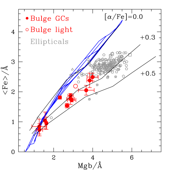
Figure 1: ${\textrm{Mg}}\,b$ indices vs. average iron $\langle{\textrm{Fe}}\rangle$ indices of galactic and Bulge GCs of our sample (large red filled symbols). The open circle shows the average value of 15 Bulge fields located in Baade’s window. Small open grey symbols show the central values of the indices for ellipticals taken from the literature: the field and cluster ellipticals from Beuing et al. (2002, pentagons); the Coma ellipticals from Mehlert et al. (2000, stars); the Fornax ellipticals of Kuntschner & Davies (1998, squares); the field and Virgo ellipticals of González (1993, triangles). Standard SSP models with metallicities $[{{\rm Z}/{\rm H}}]=(-2.25,\leavevmode\nobreak\ -1.35,\leavevmode\nobreak\ -0.55,\leavevmode\nobreak\ -0.33;\leavevmode\nobreak\ 0.00;\leavevmode\nobreak\ +0.35;+0.67)$, from bottom to top, and ages $3$, $5$, $10$, $12$ and $15$ Gyr, from left to right, are shown as blue lines. The thick black lines show 12-Gyr SSP models with same total metallicities, and various $[\alpha/{\rm Fe}]=0,\leavevmode\nobreak\ +0.3,\leavevmode\nobreak\ +0.5$ (Thomas et al. 2002b).

Fig. 1 also shows the central values (i.e. those obtained with apertures $R\sim 1/8\div 1/10\leavevmode\nobreak\ R_{e}$) of the indices of field and cluster ellipticals taken from various sources in the literature (see caption). The indices of ellipticals occupy a relatively narrow range in $\langle{\textrm{Fe}}\rangle$ and a large range in ${\textrm{Mg}}\,b$, stretching from the standard models to the high metallicity extension of the GCs sequence, and beyond. With very few exceptions, both ${\textrm{Mg}}\,b$ and $\langle{\textrm{Fe}}\rangle$ indices are measured stronger in the nuclei of ellipticals than in the most metal rich GCs in our sample. The stellar populations in the centers of ellipticals seem to be characterized by:

(i) a supersolar total metallicity;

(ii) a range in abundance ratios, from almost solar, to $[\alpha/{\rm Fe}]$ values as large as those of the most metal rich bulge clusters, or even more.

Similar conclusions have been proposed in the literature (Worthey et al. 1992; references in Introduction). Yet, these were based on the assumptions that standard models reproduce the indices of solar abundance ratios SSPs (at least at solar metallicity and above), that ${\textrm{Mg}}\,b$ and $\langle{\textrm{Fe}}\rangle$ trace the Mg and Fe abundance, and that an $\alpha$- element overabundance affects the indices in the appropriate direction.

Our comparison of the GCs data with the ellipticals, and especially the inclusion of the indices of the metal rich clusters in the galactic Bulge and the bulge field, confirm the validity of these assumptions, the clusters being used as empirical SSPs.

This empirical evidence motivates the construction of new SSP models with various, well-defined $[\alpha/{\rm Fe}]$ ratios which are shown in Fig. 1 as thick black lines (Thomas et al. 2002b, hereafter TMB02). The GCs are now very well represented by a coeval (12 Gyr old) sequence of models with various metallicities and $[\alpha/{\rm Fe}]=+0.3$, in agreement with the results from stellar spectroscopy. Note that at low metallicities (${\textrm{Mg}}\,b<2$) the standard models (blue lines) match with the enhanced models. This is due to the standard calibrations by Worthey et al. (1994) being $\alpha$-enhanced at sub-solar metallicities (Sect. 5; see also TMB02).

In the next Sect. we conduct a thorough analysis of the standard SSP models, with the aim of assessing whether effects other than an enhanced $[\alpha/{\rm Fe}]$ ratio can explain the deviation of the data from the standard models. In other words, we investigate the uniqueness of the “magnesium overabundance” solution.

5 Model Lick indices: key ingredients and ambiguities

In the model SSPs, the line-strength of an absorption line with bandpass $\Delta$ $I^{\rm SSP}$ is given by

$$I=\Delta\cdot(1-{F{\rm{}_{l}}/F{\rm{}_{c}}}),$$ (1)

where $F{\rm{}_{l}}$ and $F{\rm{}_{c}}$ are the fluxes in the absorption line and in the continuum, respectively.

In case of Lick indices this formula cannot be applied straightforwardly because of the different spectral resolution of the Lick system ($\sim 8$ Å) and of the model atmospheres (Kurucz-based stellar atmospheres have resolutions of 20 Å in the optical region where the Lick indices are defined). Basically, the problematic quantity is the flux in the absorption line $F{\rm{}_{l}}$ , because it depends on the spectral resolution. To overcome this problem, the Lick group has measured the Lick indices on observed stellar spectra having the required resolution (Burstein et al. 1984; Faber et al. 1985). Assigning to each star of their sample the values for the stellar parameters surface gravity ($g$), effective temperature ($T_{\rm eff}$) and chemical composition, they have constructed polynomial best-fitting functions which describe the various Lick indices measured on the stars, $I{\rm{}^{*}}$, as a function of these parameters, i.e. $I{\rm{}^{*}}={\mathrm{f}}(T_{\rm eff};g;[{{\rm Fe}/{\rm H}}])$. These polynomial fittings following Gorgas et al. (1993) are called fitting functions (hereafter FFs).

The integrated Lick index of an SSP model is then evaluated as it follows.

The flux in the absorption line of the generic $\mathrm{i}$-th star of the SSP, ${F{\rm{}_{l,i}^{*}}}$ , can be expressed with Eq. 1 as:

$$F{\rm{}_{l,i}^{*}}=F{\rm{}_{c,i}^{*}}\cdot(1-I{\rm{}_{i}^{*}}/\Delta)$$ (2)

where $I{\rm{}_{i}^{*}}$  that is the index of the $i$-th star is computed by inserting in the FFs the values of ($T_{\rm eff}$;$g$; chemical composition) of the $i$-th star, and $F{\rm{}_{c,i}^{*}}$ is its continuum flux. The latter is computed by linearly interpolating to the central wavelength of the absorption line, the fluxes at the midpoints of the red and blue pseudocontinua flanked to the line (Table 1 in Worthey et al. 1994). Eq. 1 can be re-written as:

$$I^{\rm SSP}=\Delta\cdot(1-{{\sum_{\rm i}F{\rm{}_{l,i}^{*}}}/{\sum_{\rm i}F{\rm{}_{c,i}^{*}}}})=\bf{{\sum_{\rm i}I{\rm{}_{i}}^{*}}}\cdot{f_{c,i}^{*}}$$ (3)

where $f_{\mathrm{c,i}}^{*}$ are the contribution of each individual star to the total continuum flux of the SSP. Thus, the SSP integrated index $I^{\rm SSP}$ is the weighted average of the stellar indices $I{\rm{}^{*}}$ with the weigths being $f_{\mathrm{c,i}}^{*}$. When computing actual models, the isochrone representing the SSP is binned in $T_{\rm eff}$ subphases, small enough to ensure that $I{\rm{}_{i}}^{*}$ is the same for the stars belonging to the given subphase. A good binning is $\Delta T_{\rm eff}\sim 100\leavevmode\nobreak\ \mathrm{K}$ (Maraston 1998). Eq. 3 can re-expressed for the subphases $j$

$$I^{\rm SSP}={{\sum_{\rm j}I{\rm{}_{j}}^{*}}}\cdot{f_{c,j}^{*}}$$ (4)

where $f^{*}_{\mathrm{c,j}}=\sum_{\mathrm{i}\in j}f_{\mathrm{c,i}}^{*}$.

It should be noted that since the rôle of the stellar continua is that of a weight, it is not crucial that they are evaluated on Kurucz-type spectra. A relation similar to Eq. 4 holds for indices measured in magnitudes (e.g. ${\textrm{Mg}}_{2}$):

$$10^{-0.4\cdot{\textrm{Mg}}_{2}^{\rm SSP}}={{\sum_{\rm j}{\rm 10^{-0.4\cdot{\textrm{Mg}}_{2}^{*}{{\rm{}_{j}}}}}}}\cdot{f_{c,j}^{*}}$$ (5)

The two ingredients ($I{\rm{}_{j}}^{*}$ and $f_{c,j}^{*}$) are discussed comprehensively in the following subsections.

5.1 Interplay between fitting functions $I{\rm{}^{*}}$and continua

To explore the systematic effects introduced in SSP models by the use of different sets of FFs, and following Maraston et al. (2001b), we compute the same SSP models with three formulations for the FFs from the literature, i.e. by Worthey et al. (1994, hereafter Worthey et al. FFs), Buzzoni et al. (1992, 1994, hereafter Buzzoni et al. FFs), and Borges et al. (1995, hereafter Borges et al. FFs).

Worthey et al. FFs, the most widely used in the SSP models in the literature, are based on the Lick sample of $\sim$ 400 nearby stars. Buzzoni et al. FFs are based on a smaller sample of stars ($\sim$ 87), also located in the solar vicinity. As is well known, the $\alpha$ to Fe abundance ratios in nearby stars vary with metallicity, ranging from the super-solar values in the Halo stars ($[\alpha/{\rm Fe}]\sim+0.3$) to the solar proportions in the metal-rich disk stars ($[\alpha/{\rm Fe}]=0.0$) (e.g. Wheeler et al. 1989; Edwardsson et al. 1993; Fuhrmann et al. 1995; Fuhrmann, 1998; see the comprehensive review by McWilliam 1997). Thus, likely, these two sets of FFs reflect $\alpha$ enhanced mixtures at low $Z$, and solar ratios at high metallicity, a trend which is dragged into the SSP models through $I{\rm{}_{j}}^{*}$ (Eqs. 4-5). This explains why the standard models in Fig. 1 (blue lines) represent well the indices of metal poor GCs.

Borges et al. FFs (see also Idiart & de Freitas Pacheco 1995) have been derived from a sample of roughly 90 stars for which the Mg to Fe ratio has been measured. Thus, they include the [Mg/Fe] ratio as an additional variable besides temperature, gravity and metallicity.

In the following subsections we discuss separately high metallicity (Sect. 5.1.1) and low metallicity (Sect. 5.1.2) model indices.

5.1.1 The metal-rich zone

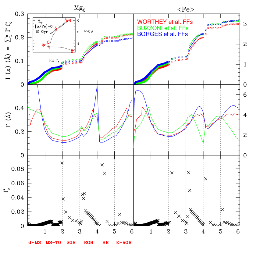
Figure 2: Closer look to model ${\textrm{Mg}}_{2}$ (left-hand panels) and $\langle{\textrm{Fe}}\rangle$ (right-hand panels) indices of a 15 Gyr old SSP with solar metallicity, solar abundance ratios, and Salpeter IMF. The upper panels show the cumulative SSP indices $I^{\mathrm{SSP}}(x)$, integrated up to the point $x$ along the isochrone (see text): $x=1$: lower Main Sequence (d-MS) up to $T_{\rm eff}\leq 5000\leavevmode\nobreak\ {\mathrm{K}}$; $x=2$: Main Sequence up to Turn Off (TO); $x=3$: Sub Giant Branch (SGB); $x=4$: Red Giant Branch (RGB); $x=5$: Horizontal Branch (HB); $x=6$: Early Asymptotic Giant Branch (E-AGB). These phases are identified on the corresponding isochrone (small inserted panel), shown in the temperature-gravity plane. Here the label $[\alpha/{\rm Fe}]=0$ refers to the composition of the stellar tracks. Colors code the different FFs for $I{\rm{}_{j}}^{*}$ (Eq. 4-5) adopted for the SSP models, by Worthey et al. (red lines), Buzzoni et al. (green lines) and Borges et al. (blue lines). The values $I{\rm{}_{j}}^{*}$ are shown in the middle panels, with lines connecting the stellar indices of the subphases along the isochrone. Finally the lower panels display the contributions of the various subphases to the total continuum flux, $f{\rm{}_{c,j}^{*}}$ (Eq. 4-5). Note that the flux contributions in post-MS ($x>2$) take into account the fuel consumption, i.e. the product of the stellar lifetimes with the stellar luminosities. For example the contribution of the long lasting RGB bump phase (peak in phase 3-4) is much larger than that of the RGB-tip (end of phase 4), where, in spite of larger stellar luminosities, the evolutionary timescale is much shorter.

Fig. 2 illustrates the interplay between $I{\rm{}_{j}}^{*}$ and $f{\rm{}_{c,j}^{*}}$ (Equation 4-5) in determining the SSP magnesium and iron indices in the particular case of a 15 Gyr, solar metallicity and solar abundance ratio SSP, with Salpeter IMF. The three sets of FFs considered are color coded as marked in the top-right panel. The $x$-axis is a monothonic coordinate along the SSP isochrone. The integer values of $x$ (1 to 6) mark the end of the six main evolutionary phases (see the caption and the figure with the isochrone inserted in the top-left panel). Each $x$-point in Main Sequence ($x\leq 2$) represents the subphase along the Main Sequence isochrone. Each $x$-point in post-MS ($x>2$) represents the $j$ subphases of every post-MS major phase, which are equally spaced in effective temperature ($\Delta T_{\rm eff}\sim 100\leavevmode\nobreak\ {\mathrm{K}}$ , Maraston 1998). The top panels show the cumulative ${\textrm{Mg}}_{2}$($x$) (left) and $\langle{\textrm{Fe}}\rangle$($x$) (right) along the isochrone, which assumes the value of the SSP model at $x=6$. As in Eq. 4-5, each value of ${\textrm{Mg}}_{2}$($x$) and $\langle{\textrm{Fe}}\rangle$($x$) is obtained by summing up to point $x$, the product of $I{\rm{}_{j}}^{*}$ times $f{\rm{}_{c,j}^{*}}$. These are separately shown in the central and lower panels, respectively. The behavior of $I{\rm{}_{j}}^{*}$ in the central panels reflects the changing of $T_{\rm eff}$ along the isochrone, both ${\textrm{Mg}}_{2}$ and$\langle{\textrm{Fe}}\rangle$  indices being very strong in cool stars.

The three sets of FFs correspond to quite different values for $I{\rm{}^{*}}$ along the isochrone, particularly in the faint dwarf regime ($x\,\hbox to0.0pt{\lower 2.5pt\hbox{$\sim$}\hss}\raise 1.5pt\hbox{$<$}\,1$), at the Tip of the RGB ($x\sim 4$), and at the end of the E-AGB ($x\sim 6$). In spite of that, the SSP indices keep very close along the isochrone, and assume quite similar total values, due to the low contribution to the total continuum flux of these particular phases. Thus, the indices turn out to be quite insensitive to the adopted set of FFs.

As a result of the weighting through $f{\rm{}_{c,j}^{*}}$, the lower MS, RGB and E-AGB bright stars (which have very strong ${\textrm{Mg}}_{2}$) are not important in determining the total SSP index. The most important contributors to the continuum fluxes in the two windows of ${\textrm{Mg}}_{2}$ and $\langle{\textrm{Fe}}\rangle$ are: the stars around the TO; those on the fainter portion of the RGB (especially at the so-called bump), and the Horizontal Branch stars. Their indices dominate the integrated values. This applies in general to old ($\,\hbox to0.0pt{\lower 2.5pt\hbox{$\sim$}\hss}\raise 1.5pt\hbox{$>$}\,\leavevmode\nobreak\ 3\leavevmode\nobreak\ {\mathrm{Gyr}}$) stellar populations, as the relative contribution to the total optical flux of the different phases does not depend much on age in this age range (Renzini & Buzzoni 1986, Maraston 1998).

Table 2: Relative contributions of stellar evolutionary phases, to the continuum flux of the ${\textrm{Mg}}_{2}$ index ($\lambda\sim 5175$Å) and $\langle{\textrm{Fe}}\rangle$ ($\lambda\sim 5300$Å), for 15-Gyr old SSPs with Salpeter IMF, and metallicities: $Z_{\odot}$ and $Z=10^{-4}$. RGB tip is the portion within 1 mag from the tip.

	$Z_{\odot}$		$10^{-4}$$Z_{\odot}$
phase	${\textrm{Mg}}_{2}$	$\langle{\textrm{Fe}}\rangle$	${\textrm{Mg}}_{2}$	$\langle{\textrm{Fe}}\rangle$
d-MS	0.11	0.13	0.10	0.10
MS TO	0.32	0.22	0.26	0.26
SGB	0.05	0.12	0.10	0.10
RGB	0.29	0.30	0.28	0.28
RGB-tip	0.01	0.01	0.10	0.10
HB	0.17	0.17	0.12	0.12
E-AGB	0.05	0.05	0.04	0.04

The contributions to the total continua of ${\textrm{Mg}}_{2}$ and$\langle{\textrm{Fe}}\rangle$ of the various evolutionary phases are given in Table 2 for 15 Gyr old metal-rich and metal-poor SSPs.

As apparent in Fig. 2, Borges et al. FFs provide $I{\rm{}_{j}}^{*}$ for faint dwarfs which are much larger than those of the other two sets. These result from the exponential increase with decreasing $T_{\rm eff}$ of their FF for ${\textrm{Mg}}_{2}$. In the validity range as specified by the authors ($T_{\rm eff}$$\,\hbox to0.0pt{\lower 2.5pt\hbox{$\sim$}\hss}\raise 1.5pt\hbox{$>$}\,3800\leavevmode\nobreak\ {\mathrm{K}}$), the FF for ${\textrm{Mg}}_{2}$ yields values as high as 1.9 mag (corresponding to 0.83 Å in the units of Fig. 2), while the coolest dwarf in their observed sample has ${\textrm{Mg}}_{2}=0.45$ mag (or 0.34 Å). These very strong (extrapolated) ${\textrm{Mg}}_{2}$ indices as obtained with a blind use of the FFs are extremely unrealistic. This example illustrates the importance of checking the behaviour of the algebraic FFs when computing SSP models.

We conclude that the Mg-Fe relation of standard models around solar metallicity (Fig. 1) is independent of the fitting functions.

5.1.2 The metal-poor zone

As shown in the previous paragraph, the differences in the FFs appear to be unimportant at $\sim Z_{\odot}$. Actually, the ${\textrm{Mg}}_{2}$ index obtained with the Borges et al. FFs does deviate from the other two values, by an amount which is comparable to the typical observational error affecting the GC data ($\sim 0.01$). This discrepancy becomes more pronounced at very low metallicities, which is relevant for the model calibration with GCs.

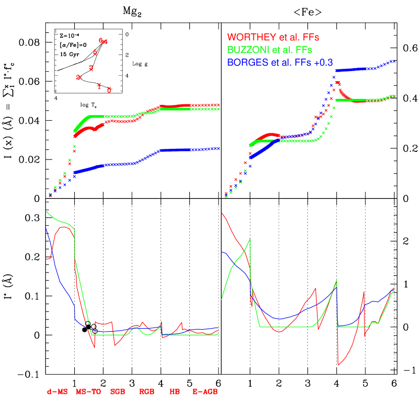
Figure 3: Same as Fig. 2 but for a very metal-poor SSP with metallicity $Z=10^{-4}$. Note that the integrated ${\textrm{Mg}}_{2}$ is made up by the lower Main Sequence (d-MS, phase 1). The symbols in the left-hand bottom panel are the values of ${\textrm{Mg}}_{2}$ of the stars in the Lick sample (filled) and in the sample used by Borges (open) with metallicities and gravities appropriate to the MS of these SSP models. As in Fig. 2, the label $[\alpha/{\rm Fe}]=0$ in the inserted panel refers to the composition of the stellar tracks.

Fig. 3 is the analogous of Fig. 2, but for a very metal-poor SSP with metallicity $Z=10^{-4}$. We use here the Borges et al. FFs with [Mg/Fe]=0.3 which is appropriate at low metallicities.

At low metallicity the temperature distribution of the isochrone shifts to hotter values (see inserted panels in Fig.s 2 and 3). The relative contributions to the continuum flux of the different evolutionary phases is very similar to the $Z_{\odot}$  case (see Table 2), but the stellar indices are now very weak, and the strongest ${\textrm{Mg}}_{2}$ are found on the lower MS, which is the coolest portion of the isochrone. As a result, the total ${\textrm{Mg}}_{2}$ of the SSP is very close to the value attained already at the turn-off point. Borges et al. FFs yield much lower stellar indices for the lower MS, compared to the other two FFs, which explains the lower integrated index. Incidentally, this is true also when adopting [Mg/Fe]=0. in the FF formula. It should be noted that the behaviour of the FFs at the low Main Sequence (phase 1) is not constrained by stellar data. Indeed, only 5 main sequence stars (symbols in the lower left panel of Fig. 3) are found at $[{{\rm Fe}/{\rm H}}]\approx-1.8$ by merging both the Lick and the Borges et al. data base. An improvement of present low-metallicity SSP models can be gained by implementing the stellar libraries with cool, dwarf and low metallicity objects.

The importance of the (lower) main sequence phase on the integrated ${\textrm{Mg}}_{2}$ has the consequence of making this index sensitive to the mass function of the stellar population. This complicates the comparison of the models with the GC data, for which the present day mass function derives from the IMF plus the possible dynamical evolution, which can lead to the evaporation of the low mass stars (e.g. Piotto & Zoccali 1999).

Different from the ${\textrm{Mg}}_{2}$ index, an important contribution to the total $\langle{\textrm{Fe}}\rangle$ index comes from the RGB portion of the isochrone, where the FFs are very noisy (see right panels in  3). Notice that the index computed with Worthey et al. FFs converges to that based on Buzzoni FFs because of negative stellar indices predicted for the hot HB stars. It is very difficult to assess the reliability of the indices as metallicity indicators at such low-$Z$.

5.2 IMF effects

As discussed in the previous sections, ${\textrm{Mg}}_{2}$ indices are very strong in dwarf stars, therefore dwarf-dominated stellar population could in principle allow to reach the very high values of ${\textrm{Mg}}_{2}$ shown by ellipticals.

Figure 4: Effect of a dwarf-dominated IMF on the ${\textrm{Mg}}_{2}$ and$\langle{\textrm{Fe}}\rangle$ diagram of SSPs. The model grid for the Salpeter IMF exponent of 2.35 is the same as in Fig. 1. The two additional solid lines are dwarf-dominated SSPs with IMF’s exponents of 4 and 5, respectively. These SSPs have 12 Gyr and metallicities as indicated by the labels. Data of GCs and ellipticals as in Fig. 1.

Fig. 4 shows the location of such dwarf-dominated SSPs in the ${\textrm{Mg}}_{2}$ vs. $\langle{\textrm{Fe}}\rangle$ diagram (lower solid lines). Lines connect 12 Gyr old models with metallicities from 3 time to half solar, and IMF’s exponents of 4 and 5 (in the notation in which Salpeter is 2.35), from top to bottom, respectively. Worthey et al. FFs have been used for this exercise. Data of ellipticals and GCs are the same as in Fig. 1.

Dwarf-dominated stellar populations are able to reproduce the ${\textrm{Mg}}_{2}$ and $\langle{\textrm{Fe}}\rangle$ indices of ellipticals without invoking abundance effects. It should be noted that in such dwarf-dominated SSPs, $>70\%$ of the total luminosity is made up by stars close to the H-burning limit. The different slope of these SSP models on the ${\textrm{Mg}}_{2}$$-$ $\langle{\textrm{Fe}}\rangle$ plane reflects the different dependence of the stellar indices from $T_{\rm eff}$ at the lower end of the MS.

These extreme IMFs are also able to reproduce the low values of the Calcium triplet absorption line at 8600 K observed in ellipticals (Saglia et al. 2002), because its strength decreases with increasing gravity (Jones et al. 1984). However, these models fail at explaining other spectral properties of ellipticals. In fact the corresponding stellar mass-to-light ratios become much larger ($M/L_{B}>\leavevmode\nobreak\ 30$, see Maraston 1998) than the dynamical ones observed in the central portions of ellipticals ($M/L_{B}\sim 6$, Gerhard et al. 2001). Similarly, a dwarf-dominated elliptical galaxy light was excluded given the strength of the CO absorption (Frogel et al. 1978) and the absence of the Wing Ford bands in absorption (Whitford  1977). The case of such a dwarf-dominated present mass function for GCs, and the Bulge field is ruled out by direct observations of the lower MS (de Marchi & Paresce 1997; Piotto & Zoccali 1999; Zoccali et al. 2000a).

We conclude that an extremely steep IMF is not a viable alternative to explain the high values of the Mg indices in ellipticals.

5.3 The effect of stellar evolutionary tracks

As already stated, our standard SSP models are based on the stellar tracks by Cassisi et al. (1999). Since differences exist among different sets of tracks, it is interesting to check their impact on the model indices. To this aim we have computed SSP models with Worthey et al. FFs, but varying the input tracks. The Padova stellar tracks and isochrones as available on the Web have been used, specifically those by Fagotto et al. (1994) for metallicities $[{{\rm Z}/{\rm H}}]=-1.69$ and $-0.69$, and those by Salasnich et al. (2000), with solar scaled abundance ratios, for metallicities $[{{\rm Z}/{\rm H}}]=-0.4,0,0.35$. The fuel consumption theorem is adopted also for these SSPs, following the method described in Maraston (1998; 2003).

Figure 5: Effect of stellar tracks on the Lick indices of 12 Gyr SSPs models with various total metallicities $[$Z/H]. Filled symbols: SSPs adopting the Cassisi tracks, open symbols: SSPs adopting the Padova tracks.

The results are shown in Fig. 5, which compares the ${\textrm{Mg}}\,b$ and $\langle{\textrm{Fe}}\rangle$ indices of 12 Gyr SSP models as a function of the total metallicities $[$Z/H], as obtained with the Cassisi tracks (filled circles) and the Padova tracks (open circles),

The use of the Padova tracks produces slightly stronger ${\textrm{Mg}}\,b$ indices, at metallicities $[$Z/H] between $\sim-0.5$ and solar. This effect is most likely due to the cooler temperatures of the Padova tracks along the Red Giant Branch with respect to the Cassisi tracks (see also Maraston 2003). A very modest impact is present also for the $\langle{\textrm{Fe}}\rangle$ index. Note that at metallicities above solar the $\langle{\textrm{Fe}}\rangle$ obtained with the Padova tracks is stronger than that obtained with the Cassisi tracks, while the corresponding ${\textrm{Mg}}\,b$ indices are consistent. This implies that the discrepancy with ellipticals data is slightly larger when the Padova tracks are used. The differences are however very small, and the conclusions drawn from Fig. 1 are not affected by our use of a specific set of stellar tracks.

Recently, isochrones and tracks with super-solar $[\alpha/{\rm Fe}]$ ratios became available (Salasnich et al. 2000 with $[\alpha/{\rm Fe}]=+0.3$; see also Bergbusch & VandenBerg 2001; Kim et al. 2002). These improved upon previous calculations that considered only the effect on nuclear reaction rates (e.g. Salaris et al. 1993), while the updated tracks have also included the effect of $\alpha$-enhancement on the stellar opacities. Here we use the Salasnich’s computations in order to check the impact of $\alpha$-enhanced tracks on the final index values of SSP models. For consistency, we compare the indices based on the two Padova sets, with solar scaled and $\alpha$-enhanced abundance ratio.

Figure 6: Effect of $\alpha$-enhanced stellar tracks on ${\textrm{Mg}}_{2}$ , ${\textrm{Mg}}\,b$, $\langle{\textrm{Fe}}\rangle$ and ${\textrm{H}}\beta$ of 10 Gyr SSPs (Salpeter IMF) with various total metallicities $[$Z/H]. Dotted lines: solar-scaled tracks. Solid lines: $[\alpha/{\rm Fe}]=+0.3$ tracks. Tracks are from Salasnich et al. (2000), the Worthey FFS are adopted.

This is shown in Fig. 6 for the illustrative case of 10 Gyr old SSPs.

For the same total metallicity $[$Z/H], the Mg and Fe indices of SSPs based on $\alpha$-enhanced stellar tracks (solid lines) are lower than those based on solar scaled stellar tracks (dotted lines), This happens because the $\alpha$-enhanced tracks are bluer than the solar-scaled ones at fixed total metallicity (Salasnich et al. 2000), because of the lower stellar opacities. So, by increasing $[\alpha/{\rm Fe}]$  at constant $[$Z/H] the Mg indices actually decrease!

This rather counterintuitive behavior is a consequence of the fact that, at given total metallicity, the increase of the $[\alpha/{\rm Fe}]$ ratio produces only a small increase of the $\alpha$ elements, and instead a large decrease of iron. In fact, in solar proportions the total metallicity is by far dominated by the $\alpha$-elements ($\sim 74\%$ by mass), the iron-peak elements amounting only to $\sim 8\%$, the residual being contributed by elements produced by the p, s, and r processes (Trager et al. 2000; TMB02).For example, compared to solar proportion in a mixture with $[\alpha/{\rm Fe}]$=+0.3 the $\alpha$ elements will contribute slightly more than $\sim 74\%$, but the iron peak elements will be reduced by almost a factor of two, down to $\sim 4\%$. Therefore, the main effect is to decrease iron rather than to increase, e.g., magnesium. Since iron is the most effective electron donor (e.g. Salasnich et al. 2000), the lower abundance of iron in enhanced $[\alpha/{\rm Fe}]$ mixtures has the effect of decreasing their low-temperature opacities, which in turn determine an increase of the temperature of the RGB, and finally a decrease of the Mg indices because these are stronger in cool stars.

The bluing of the isochrone also affects the ${\textrm{H}}\beta$ line indices, which are stronger when $\alpha$-enhanced tracks are adopted (Fig. 6, upper right panel). Therefore, in order to reproduce the observed ${\textrm{Mg}}_{2}$, $\langle{\textrm{Fe}}\rangle$  and ${\textrm{H}}\beta$  indices, the $\alpha$-enhanced tracks require older ages.

It should be noted that for the models of Fig. 6, the parameter expressing the chemical composition in the Worthey et al. FFs (referred to as $[$Fe/H] in Worthey et al. 1994) has been considered to represent the total metallicity. As discussed in Sect. 3, this might be not entirely correct, since a variety of methods have been used, both photometric and spectroscopic, to determine such parameter for the stars of the Lick sample. If the $[$Fe/H]’s values are used, the metallic indices shown in Fig. 6 decrease even further.

Fig. 6 illustrates that accounting only for $\alpha$-enhanced stellar tracks to compute $\alpha$-enhanced SSP models, while using the same FFs, affects the indices in the wrong direction with respect to the locus occupied by the metal-rich GCs and ellipticals data in Fig. 1 (${\textrm{Mg}}_{2}$ is affected more than $\langle{\textrm{Fe}}\rangle$). A fully consistent exploration of the effect of the $[\alpha/{\rm Fe}]$ ratio requires also the use of fitting functions depending on $[\alpha/{\rm Fe}]$. This is done in TMB02.

5.4 Summary

The conclusions of the previous paragraphs are the following.

1. Differences in the available sets of FFs do not affect the integrated ${\textrm{Mg}}_{2}$  and $\langle{\textrm{Fe}}\rangle$ indices, due to the low contribution to the total continuum flux of those evolutionary phases where the FFs are mostly discrepant.

2. For both ${\textrm{Mg}}_{2}$ and $\langle{\textrm{Fe}}\rangle$ (and in general indices measured in the optical) the most important contributors are MS TO, RGB and HB stars. These are the evolutionary phases where the FFs need to be best constrained from stellar data.

3. Results 1 and 2 hold for metallicities $[{{\rm Fe}/{\rm H}}]\,\hbox to0.0pt{\lower 2.5pt\hbox{$\sim$}\hss}\raise 1.5pt\hbox{$>$}\,-1$, and are largely independent of the age and stellar tracks used.

4. At very low metallicities (less than $Z_{\odot}$/10) the lower MS appears to dominate the value of the SSP ${\textrm{Mg}}_{2}$ index. Uncertainties in the FFs and in the mass function jeopardize the calibration of the theoretical indices with the GC data.

5. At metallicities  $\sim$$>$ $Z_{\odot}$/2, the slope of the solar scaled ${\textrm{Mg}}_{2}$ vs $\langle{\textrm{Fe}}\rangle$ relation for SSP models seems quite robust. One possibility to get strong ${\textrm{Mg}}_{2}$ indices in combination with weak $\langle{\textrm{Fe}}\rangle$  without invoking a super-solar $[\alpha/{\rm Fe}]$, is to adopt a very steep exponent for the IMF. However, IMF exponents as large as 4 $\div$ 5 have to be used in order to encompass the locus occupied by ellipticals. Such values are ruled out by other constraints.

6. When $\alpha$ enhanced tracks are used the ${\textrm{Mg}}_{2}$ and $\langle{\textrm{Fe}}\rangle$ indices become $weaker$, due to the $blueing$ of the isochrone. Therefore, in order to match the observational data of GCs and ellipticals, abundance effects have to be accounted also in the FFs.

6 Model Lick indices: comparison with the data

In this section we compare quantitatively the indices for our sample of GCs with the models. Good models have to fulfill two requirements: i) the metallicities obtained using different line-strengths have to be consistent; ii) the metallicities derived from the models have to be in agreement with those determined independently from, e.g. spectroscopy of stars in GCs or CMD fitting. We already know from Fig. 1 that condition i) will not be fulfilled at $[{{\rm Z}/{\rm H}}]\,\hbox to0.0pt{\lower 2.5pt\hbox{$\sim$}\hss}\raise 1.5pt\hbox{$>$}\,-0.6$, because the GCs data deviate from the models. It is however important to check quantitatively the discrepancy. For a comparison of the standard SSP models used here with Magellanic Clouds clusters, we refer to Beasley et al. (2002).

In this section we also explore the significance of other Lick indices as metallicity indicators. Finally we calibrate the Balmer lines.

6.1 Chemical compositions from Mg and Fe indices

Figure 7: Comparison between the SSP-derived total metallicities from ${\textrm{Mg}}_{2}$ (left-hand panel) and $\langle{\textrm{Fe}}\rangle$ (central panel) for our sample of GCs, with the empirical metallicity scale $[$Fe/H] as compiled by Harris (1996), which is largely based on the Zinn & West (1984) scale. The standard SSPs, i.e. those based on Milky Way calibrated FFs, used here adopt the Cassisi tracks and: the Worthey et al. FFs (open circles), the Buzzoni et al. FFs (open triangles), the Borges et al. FFs (asterisks). The age of these SSPs is 12 Gyr. The SSP-derived $[$Z/H] is obtained by interpolating the observed indices on the model grid, separately. Diagonal lines show the 1 to 1 relations. In the right hand-panel the $\langle{\textrm{Fe}}\rangle$ index of the SSP models is derived by plugging $[$Fe/H] in the FFs instead of the total metallicity $[$Z/H](see Sect. 3), for the only case of the Worthey et al. FFs.

Fig. 7 compares the metallicities $[$Z/H] derived from the standard SSP models, with those provided by the revised compilation of Harris (1996), which is largely based on the Zinn & West (1984) scale, for each GC of our sample. The model $[$Z/H] is obtained by interpolating the ${\textrm{Mg}}_{2}$ index (left-hand panel) and the $\langle{\textrm{Fe}}\rangle$ index (central panel) on the SSP models (12 Gyr) based on the Cassisi tracks plus the FFs by: Worthey et al. (open circles), Buzzoni et al. (triangles), and Borges et al. (asterisks). The errorbars connect the minimum and maximum model metallicities obtained by subtracting (adding) the observational errors to the measured values. For the empirical metallicities, a conservative error of +0.2 dex has been considered. The right-hand panel refers to a model $\langle{\textrm{Fe}}\rangle$ index as obtained by using as a metallicity input in the Worthey et al. FFs, the value of the iron abundance $[$Fe/H] and assuming an $[\alpha/{\rm Fe}]=+0.3$ (see Sect. 3). Also in this case, the interpolation is with the model total metallicity $[$Z/H].

Fig. 7 shows that for standard SSP models:

i) the total metallicities $[$Z/H] as derived from the ${\textrm{Mg}}_{2}$ index (left-hand panel) are well consistent with the empirical scale of Zinn & West at metallicities lower than $\sim-0.5$. For NGC 6553 and NGC 6528 the models give $[$Z/H] values somewhat in excess of the values on the Zinn & West scale, but would agree with the near solar abundance indicated by the spectroscopic observations (Barbuy et al. 1999; Cohen et al. 1999).

ii) the total metallicities $[$Z/H] as derived from the $\langle{\textrm{Fe}}\rangle$ index, when the latter is computed with $[$Z/H] as input of the FFs (central panel), are systematically lower than the empirical ones, by roughly 0.3 dex.

iii) the total metallicities $[$Z/H] as derived from the $\langle{\textrm{Fe}}\rangle$ index, when the latter is computed by using instead the iron abundance $[$Fe/H] and assuming a 0.3 dex $\alpha$-enhancement as input of the FFs (right-hand panel) is consistent with the Zinn & West values.

On the basis of these evidences we conclude that:

i) the standard SSP models, i.e. those based on the Milky Way calibrated FFs, do not underestimate the ${\textrm{Mg}}_{2}$ index; rather they overestimate the $\langle{\textrm{Fe}}\rangle$ index. The disagreement between the models and the GC (and ellipticals) data would then point towards an iron deficiency, as opposed to magnesium enhancement, at virtually all metallicities. Suggestions in this direction can be found in Buzzoni et al. (1994), Trager et al. (2000), TMB02;

ii) the model-derived total metallicities $[$Z/H] are in agreement with the metallicities on the Zinn & West scale which are referred as to $[$Fe/H] (see Sect. 3.1).

In the left-hand panel of Fig. 7 two of the four clusters at $[{{\rm Fe}/{\rm H}}]_{\mathrm{ZW}}\sim-1.4$ (NGC 6218 and NGC 6981) have a too low ${\textrm{Mg}}_{2}$-derived metallicity, when the Worthey et al. or the Buzzoni et al. FFs are used. The SSPs with the Borges et al. FFs, instead reproduce the ${\textrm{Mg}}_{2}$ indices of these two specific clusters, because of the lower ${\textrm{Mg}}_{2}$ indices of these FFs (see Sect. 4.2). Since at low $Zs$ the ${\textrm{Mg}}_{2}$ index is dominated by the lower MS component (Sect. 5.3), dynamical effects stripping low mass stars could be responsible for the observed low ${\textrm{Mg}}_{2}$ indices of these particular objects. Piotto et al. (2001) show that indeed the mass function of NGC 6981 is consistent with a power-law with a slope flatter than the Salpeter one. We note that NGC 6218 is the object of our sample with the poorest sampled light (paper I).

Figure 8: The metallicities of the GCs as derived from the $\alpha$-enhanced SSPs of TMB02, with age of 12 Gyr and $[\alpha/{\rm Fe}]=+0.3$. In the left-hand and central panels, the total metallicity $[$Z/H] as derived with the ${\textrm{Mg}}_{2}$ and the $\langle{\textrm{Fe}}\rangle$ index, respectively are compared with the values on the Zinn & West scale. In the right-hand panel the predicted $[$Fe/H] is compared to the empirical scale of iron abundances by Carretta & Gratton (1997).

Fig. 8 compares the metallicities of each GCs as obtained from the ${\textrm{Mg}}_{2}$ (left-hand panel) and $\langle{\textrm{Fe}}\rangle$ (right-hand panel) index using the TMB02 $\alpha$-enhanced SSP models, with 12 Gyr and $[\alpha/{\rm Fe}]=+0.3$ (solid black lines in Fig. 1). These models include the dependence of the fitting functions for $I{\rm{}^{*}}$ on the $[\alpha/{\rm Fe}]$ parameter.

The total metallicities $[$Z/H] as derived from ${\textrm{Mg}}_{2}$ and $\langle{\textrm{Fe}}\rangle$ are in excellent agreement with each other. This results from having taken a super solar $[\alpha/{\rm Fe}]$ abundance ratio in the models into account. The metallicities are in excellent agreement with those in the Zinn & West scale, over the whole range covered by our sample. The assumed $[\alpha/{\rm Fe}]=+0.3$ for the GCs is in agreement with the $[\alpha/{\rm Fe}]$ measured spectroscopically (see e.g. Carney 1996; Salaris & Cassisi 1996). For the Bulge GC NGC 6528 recent spectroscopic abundance determinations give: $Z\sim Z_{\odot}$, $[\alpha/{\rm Fe}]\sim 0.3$, $[{{\rm Fe}/{\rm H}}]\sim-0.3$ (Barbuy et al. 1999; Origlia et al. 2001). We acknowledge that some controversy exists in the literature: Carretta et al.(2001; see also Cohen et al. 1999) give $[{{\rm Fe}/{\rm H}}]\sim+0.08$ for 6528 and $[{{\rm Fe}/{\rm H}}]\sim-0.06$ for NGC 6553, $[\alpha/{\rm Fe}]\sim 0.2\div 0.4$. It would be extremely important to pin down the element abundances for these objects which are the most metal-rich calibrators available.

Carretta & Gratton (1997) provide a metallicity scale for GCs which should reflect the $[$Fe/H] abundance. The right-hand panel of Fig. 8 compares the model-derived $[$Fe/H] with this scale. The metallicities in the Zinn & West scale are transformed into the Carretta & Gratton scale by adopting the relation provided by the authors. This comparison is rather poor. On this scale the iron abundance of our GC sample appears clustered on two values, while the observed $\langle{\textrm{Fe}}\rangle$ indices span a considerable range. It seems difficult to reconcile our index-based $[$Fe/H]  with those in the Carretta & Gratton scale.

We conclude this section discussing the case of 47 Tuc, which allows us to demonstrate the importance of comparing data and models which are set on the same system (see Sect. 3.1, Table 1). If we use the indices measured in the Burstein et al. (1984) system, 47 Tuc has $[{{\rm Z}/{\rm H}}]\simeq-0.50$; if we use the indices measured in the Worthey et al. one, we get $[{{\rm Z}/{\rm H}}]\simeq-0.78$. This last value is in perfect agreement with the metallicity of 47 Tuc in the Zinn & West scale ($[{{\rm Z}/{\rm H}}]\sim-0.76$, from Harris 1996). In addition we notice that the metallicity derived for 47 Tuc using the indices in the Burstein et al. (1984) is as large as that of NGC 6356, while the comparison of the RGB ridge lines of these two clusters indicates that 47  Tuc is more metal-poor (Bica et al. 1994). For a critical discussion focused on 47 Tuc see Schiavon et al. (2002).

Table 3: The metallicities $[$Z/H] derived with ${\textrm{Mg}}_{2}$ and $\langle{\textrm{Fe}}\rangle$ of standard SSPs adopting the Worthey et al. FFs (col. 3-4), the Buzzoni et al. FFs (col. 5-6) and the Borges et al. FFs (see left-hand and central panel of Fig. 7). The adopted SSP age is 12 Gyr. The last 2 lines report the calibration of 47 Tuc, using the original data by Covino et al. (1995) and those obtained by us on their spectra by adopting the W94 index definition (see 3.2, Table 1). In Col. 2 the empirical metallicities of the GCs as given by Harris (1996) are listed.

name	$[$Fe/H]ZW	$\mathrm{[Z/H]}^{SSP}_{WFFs}$		$\mathrm{[Z/H]}^{SSP}_{BFFs}$		$\mathrm{[Z/H]}^{SSP}_{BorFFs}$
		${\textrm{Mg}}_{2}$	$\langle{\textrm{Fe}}\rangle$	${\textrm{Mg}}_{2}$	$\langle{\textrm{Fe}}\rangle$	${\textrm{Mg}}_{2}$
NGC 6981	-1.40	-1.91	-1.83	-1.87	-1.73	-1.46
NGC 6637	-0.71	-0.73	-1.05	-0.76	-0.94	-0.54
NGC 6356	-0.50	-0.51	-0.91	-0.55	-0.81	-0.35
NGC 6284	-1.32	-1.27	-1.58	-1.29	-1.41	-1.07
NGC 6626	-1.45	-1.31	-1.48	-1.33	-1.31	-1.12
NGC 6441	-0.53	-0.53	-0.80	-0.57	-0.70	-0.36
NGC 6218	-1.48	-1.80	-1.71	-1.77	-1.57	-1.35
NGC 6624	-0.56	-0.45	-0.88	-0.59	-0.78	-0.39
NGC 6388	-0.60	-0.81	-0.84	-0.84	-0.74	-0.61
NGC 5927	-0.37	-0.17	-0.65	-0.23	-0.56	-0.07
NGC 6553	-0.34	+0.05	-0.27	+0.01	-0.29	+0.11
NGC 6528	-0.17	+0.09	-0.35	+0.06	-0.35	+0.14
47 Tuc(B84)	-0.76	-0.50	-0.66	-0.53	-0.58	-0.33
47 Tuc (W94)	-0.76	-0.78	-1.07	-0.81	-0.96	-0.59

6.2 The other Lick indices as abundance indicators

In this section we check the behaviour of the other Lick indices as abundance indicators, by analysing the correlations with ${\textrm{Mg}}\,b$ and $\langle{\textrm{Fe}}\rangle$, which we have shown (Fig. 1) are likely to trace the $\alpha$ elements and the Fe abundances, respectively. To this purpose, we divide the indices into three groups: those which should be predominantly sensitive to $\alpha$-elements (${\textrm{Mg}}_{1}$,${\textrm{Mg}}_{2}$, etc.); those which should trace the Fe abundance (Fe4383; Fe5782; etc.); and the others (${\rm CN}_{1}$; ${\rm CN}_{2}$; etc.), for which the case is less clear. The correlations are checked with respect to the model predictions. The evolutionary populations synthesis of Maraston (1998, see Sect. 3) has been updated for the computations of the whole set of Lick indices given in Worthey et al. (1994), plus the higher-order Balmer lines of Worthey & Ottaviani (1997). A detailed analysis of the contributions to these indices, similar to that given in Sect. 4 for ${\textrm{Mg}}_{2}$ and $\langle{\textrm{Fe}}\rangle$, will appear in Maraston (2003).

Figure 9: Calibration of $\alpha$-sensitive Lick indices. Standard SSPs like in Fig. 1. Filled symbols denote our sample GCs, the large open symbol the average value of the Bulge light in the Baade window.

Fig. 9 shows the correlation of the first group of indices with ${\textrm{Mg}}\,b$. The Mg indices: ${\textrm{Mg}}\,b$, ${\textrm{Mg}}_{1}$ and ${\textrm{Mg}}_{2}$ are very well consistent with each other and can be used as tracers of $\alpha$-elements. The line-strength Ca4227 still appears to correlate with Mgb, although displaying slightly smaller values, while the other supposed Calcium-sensitive line Ca4455 does not. The reason for such mismatch is not clear to us. We suspect a calibration problem. The titanium-oxide indices ${\rm TiO}_{1}$ and ${\rm TiO}_{2}$ behave consistently with ${\textrm{Mg}}\,b$ at low metallicities, while at high metallicities these indices would overestimate the $\alpha$-element abundance with respect to ${\textrm{Mg}}\,b$. However, TiO is contributed by M-type stars which may be poorly treated in the models and which are present only in the metal-rich clusters.

Figure 10: Model calibration. Iron-sensitive Lick indices. Model and data like in Fig. 9.

The NaD index scales with ${\textrm{Mg}}\,b$ although with some scatter. As discussed by TMB02, the reason for the scatter is most probably the absorption by interstellar medium affecting objects close to the galactic plane. Because of this possible source of contamination the NaD index is a problematic metallicity indicator for stellar populations (see also Burstein et al. 1984).

Fig. 10 shows the second group of indices that should trace the iron abundance. Indeed, all the plotted indices correlate very well with $\langle{\textrm{Fe}}\rangle$. The models fit well most of these indices. The only exception is Fe5782, which is underpredicted by the models, suggesting an offset in the FFs. This offset most probably originates from the low signal-to-noise of the Lick/IDS data for Fe5782, which results from the extreme weakness of this line (S. Trager, private communication).

It is worth noting that the ${\rm C}_{2}$4668 index is tighly correlated to $\langle{\textrm{Fe}}\rangle$, although is supposed to trace the abundance of Carbon (see Trager et al. 1988).

Figure 11: Model calibration of remaining Lick indices. Model and data like in Fig. 9.

In Fig. 11 we plot the remaining indices vs ${\textrm{Mg}}\,b$. ${\rm CN}_{1}$ and ${\rm CN}_{2}$ seem to trace the same elements as ${\textrm{Mg}}\,b$, though with an offset, especially at high metallicity and in the ${\rm CN}_{1}$. At least part of the effect could be due to the fitting functions not incorporating stars belonging to high-metallicity GCs. As also discussed in Paper I, GCs have stronger CN indices compared to the bulge field (in Baade’s Window) at the same value of $\langle{\textrm{Fe}}\rangle$. This may be caused by GCs stars accreting the CN-rich ejecta of AGB stars. The low-density environment of the field prevents a similar accretion on field stars. Therefore the models at high metallicity are lower than GC data because the fitting functions at high metallicity are contructed with field stars.

Finally also the G-band seems to follow magnesium, but the relation is more scattered.

In Fig.s 9 to 11, the large open symbol shows the average index values of 15 Bulge fields, located in Baade Window. In all indices, the value of the Bulge field is consistent with an average metallicity close to that of the most metal-rich GCs. This is quantitatively confirmed by the detailed metallicity distribution of the bulge stars from optical-infrared color-magnitude diagrams (Zoccali et al. 2002). The large value of the NaD index for the Bulge average field is again most probably due to contamination by interstellar medium, as discussed above.

6.3 Balmer lines

Figure 12: Impact of the morphology of the Horizontal Branch on ${\textrm{H}}\beta$. Models refer to SSP ages of 10 and 15 Gyr, and $[{{\rm Z}/{\rm H}}]$ from $-2.25$ to $0.67$ as labeled in the Fig.. Solid lines show models in which no mass loss has been accounted along the RGB. The dashed lines are 15 Gyr old models in which mass-loss has been applied at metallicities $\,\hbox to0.0pt{\lower 2.5pt\hbox{$\sim$}\hss}\raise 1.5pt\hbox{$<$}\,-0.5$, in order to reproduce the observed ${\textrm{H}}\beta$ of metal poor GCs (see Maraston & Thomas 2000). The GCs of our sample are plotted according to their observed HB morphology, by means of the HBR parameter (from the Harris 1996 catalogue): pure blue HB (HBR=1, solid symbols); red HB (HBR=0, open symbols); intermediate morphologies (crosses). The open circle without errorbars shows the average value of 15 Bulge fields in Baade window. The very thick line at solar metallicity shows the locus of the solar metallicity models, as corrected to take into account the bluening of the tracks due to $\alpha$-enhancement (see Fig. 6).

As well known Balmer lines are strongest in A-type stars, and become pregressively weaker for decreasing temperatures. In synthetic stellar populations their strength is sensitive to the temperature of the main sequence turnoff, hence to the age. Therefore the Balmer line strengths are used to estimate the age of e.g. elliptical galaxies, in an attempt at breaking the age/metallicity degeneracy (e.g. Worthey et al. 1992). However, turnoff stars are not the only potential contributor to the strength of the Balmer lines: Horizontal Branch (HB) stars may be as warm or even warmer than the turnoff. Actually, the ${\textrm{H}}\beta$ index is perhaps more sensitive to the temperature distribution of the HB (the HB morphology) than to any other parameter (Worthey 1992; Barbuy & de Freitas Pacheco 1995; Greggio 1997; Maraston & Thomas 2000). Therefore, attempting to break the age/metallicity degeneracy with Balmer lines indices one runs into the age/HB morphology degeneracy. In the modeling the HB morphology cannot be derived from first principles, because of the rôle played by mass-loss on shaping the HB morphology . Additionally, possible dynamical effects (e.g. Fusi Pecci et al. 1993) may determine anomalous HB morphologies at a similar total cluster metallicity (the 2nd parameter problem in Milky Way GCs). Therefore the effect of the HB morphology to be used in SSP models needs to be calibrated on the Balmer indices.

For our models this is done in Maraston & Thomas (2000), to which we refer for more details on the model parameter. In that work the mass-loss to be applied at every SSP metallicity was calibrated in order to reproduce the ${\textrm{H}}\beta$ line of the GC sample by Burstein et al. (1984), Covino et al. (1995) and Trager et al. (1998). Here we check if those calibrated models are able to reproduce the Balmer lines measured for our sample sample.

Fig. 12 shows two sets of SSP models obtained with different prescriptions for the RGB mass loss, various metallicities and two ages (10 and 15 Gyr). Aimimg at calibrating the model Balmer lines with metallicity, we have chosen as $x$-axis the index [MgFe] . TMB02 show that this index by washing out $[\alpha/{\rm Fe}]$ effects, is able to trace total metallicity.

The solid lines connect models in which no mass loss is applied to the RGB. In this case the morphology of the HB is red (i.e., all HB lifetime is spent on the red side of the RR-Lyrae location at $\log T_{\rm eff}\sim 3.85$), except at the very low metallicity $[{{\rm Z}/{\rm H}}]=-2.25$, where the HB is spent at $\log T_{\rm eff}\,\hbox to0.0pt{\lower 2.5pt\hbox{$\sim$}\hss}\raise 1.5pt\hbox{$>$}\,3.85$ even when no mass-loss is applied. The dashed line shows the 15 Gyr SSPs with $[{{\rm Z}/{\rm H}}]\,\hbox to0.0pt{\lower 2.5pt\hbox{$\sim$}\hss}\raise 1.5pt\hbox{$<$}\,-0.5$, in which mass-loss has been applied on the RGB according to canonical prescriptions. This leads to extended HBs, with blue morphologies (i.e. the whole HB lifetime is spent the blue side of the RR-Lyrae location) at $[{{\rm Z}/{\rm H}}]=-2.25$, and intermediate HB morphologies at metallicities between $[{{\rm Z}/{\rm H}}]=-1.35$ ($\sim 84\%$ of the HB lifetime is spent blueward the RR-Lyrae) and $[{{\rm Z}/{\rm H}}]=-0.55$ ($\sim 10\%$ of HB lifetime is spent blueward the RR-Lyrae).

The cluster data are plotted according to their observed HB morphologies, (B(lue)HB: filled symbols; R(ed)HB: open symbols; I(ntermediate)HB: asterisks) by means of the HBR parameter (Harris 1996).

The calibrated models by Maraston & Thomas (2000) are able to reproduce the observed ${\textrm{H}}\beta$ of our sample GCs. In particular they reproduce the relatively strong ${\textrm{H}}\beta$ ($\sim 1.9$ Å) of NGC 6388 and NGC 6441, which are metal-rich clusters ($[{{\rm Fe}/{\rm H}}]_{\mathrm{ZW}}=-0.6;-0.53$) with an extension of the HB to the blue (Rich et al. 1997). The percentage of HB stars that is found blueward the RR Lyrae gap is: $\sim 15\%$ for NGC 6388 (Zoccali et al.  2000b) and $\sim 13\%$ for NGC 6441 (M. Zoccali, private communication). This is well consistent with the HB evolutionary timescales of the Maraston & Thomas (2000) models as given above.

Concerning the most metal-rich objects NGC 6528 and NGC 6553, their relatively strong ${\textrm{H}}\beta$ cannot be ascribed to HB effects since both clusters have a red Horizontal Branch (Ortolani et al. 1995). Part of the effect can be explained in terms of $\alpha$-enhancement at high metallicities, without invoking young ages which would be in contradictions with CMD determinations (Ortolani et al. 1995). In Sect. 5 we have shown (Fig. 6) that $\alpha$-enhanced tracks are bluer than the corresponding solar-scaled ones. As a consequence the ${\textrm{H}}\beta$  lines are higher by $0.13$ Å at solar metallicity. The thick line in Fig. 12 connects the SSP models as shifted by this amount. Note however the rather large errorbar on the ${\textrm{H}}\beta$ of NGC 6553.

The index of the average light of the Bulge is shown as an open symbol without errorbars, and sits on the $\sim$ 15 Gyr model with red HB. The low ${\textrm{H}}\beta$ line does not leave room for intermediate age stars in our sampled Bulge fields.

Figure 13: Calibration of the higher-order Balmer lines ${\textrm{H}}\delta_{A}$, ${\textrm{H}}\delta_{F}$, ${\textrm{H}}\gamma_{A}$and ${\textrm{H}}\gamma_{F}$ (Worthey & Ottaviani (1997) of the standard SSP models, see Figure 12.

Finally we calibrate the higher-order Balmer lines ${\textrm{H}}\delta_{A}$, ${\textrm{H}}\gamma_{A}$, ${\textrm{H}}\delta_{F}$ and ${\textrm{H}}\gamma_{F}$ (Worthey & Ottaviani (1997) of the same models, in Fig. 13. It can be appreciated a very good consistency between the ${\textrm{H}}\beta$and the higher-order Balmer lines.

7 Summary and Conclusions

Synthetic Lick indices (e.g., ${\textrm{Mg}}_{2}$, $\langle{\textrm{Fe}}\rangle$, ${\textrm{H}}\beta$, etc.) of stellar population models (SSP) are calibrated over a range of metallicities that extends up to solar metallicity using a sample of galactic globular clusters which includes high-metallicity clusters of the Galactic bulge. These data allow us to investigate empirically a well known property of elliptical galaxies, known as “magnesium overabundance” (Worthey et al. 1992), where the observed Mg indices in ellipticals are much stronger at given iron than predicted by standard models. By standard models we mean those constructed using stellar templates that are $\alpha$-enhanced at low metallicity but assume solar elemental proportions at high metallicity. This effect has been generally interpreted in terms of $\alpha$-enhancement of elliptical galaxies, even if the bulk of their stellar population is metal rich. However, such conclusion rests on two assumptions: i) the models that are believed to represent solar scaled elemental ratios are correct, and ii) the Lick Mg and Fe indices trace the abundance of the corresponding element.

Using our GC database we have checked empirically both assumptions by comparing the Lick indices of the GCs spectra with those of ellipticals. The result is that the magnesium and iron indices of the metal-rich GCs, of the integrated light of the Galactic bulge, and of elliptical galaxies, define a fairly tight correlation in the ${\textrm{Mg}}\,b$-$\langle{\textrm{Fe}}\rangle$diagram, with elliptical galaxies lying on the prolongation of the correlation established by the GCs, i.e., also the metal-rich GCs of the Milky Way bulge exhibit the “magnesium overabundance” syndrome. Since the GCs are indeed known to have enhanced $[\alpha/{\rm Fe}]$ ratios from stellar spectroscopy ($[\alpha/{\rm Fe}]\simeq+0.3$), we conclude that the interpretation of elliptical galaxy spectra in terms of “magnesium overabundance” is indeed correct. The comparison with the GCs further allows us to point out that, rather than “magnesium overabundance”, the enhanced $[\alpha/{\rm Fe}]$ ratio in GCs, and ellipticals is most probably the result of an iron deficiency with respect to the solar values (see Sect. 6.1). This agrees with previous suggestions (Buzzoni et al. 1994; Trager et al. 2000b) and with the recent results by TMB02. The enhanced $[\alpha/{\rm Fe}]$ ratio implies short formation timescales for the bulk stellar population, an important constraint for formation models of elliptical galaxies and bulges (e.g., Matteucci 1994; Thomas et al. 1999), which is difficult to reconcile with current semianalytic models of galaxy formation (Thomas & Kauffmann 1999).

In parallel, the comparison of the SSP model with the GC data has allowed us to shed some light on the models themselves. Around solar metallicity, the standard models are based on the stellar indices of Milky Way disk stars (by Worthey et al. 1994 or Buzzoni et al. 1992; 1994), and therefore would reproduce the indices of stellar populations with solar-scaled elemental proportions. This explains why they fail to reproduce the ${\textrm{Mg}}\,b$-$\langle{\textrm{Fe}}\rangle$correlation followed by galactic GCs and the Galactic bulge, which are characterized by elemental ratios which are specific to the Galactic spheroid. This failure was also noted by Cohen et al. (1998) for both the metal rich globulars of the Milky Way as well as for those of M87, but was not attributed to an abundance effect.

At metallicities $[{{\rm Z}/{\rm H}}]\,\hbox to0.0pt{\lower 2.5pt\hbox{$\sim$}\hss}\raise 1.5pt\hbox{$<$}\,-1.$ the standard models use metal poor template stars that belong to the galactic halo, hence have supersolar $[\alpha/{\rm Fe}]$ ratios. This explain why standard models successfully reproduce the Lick indices of the metal poor GCs, which also belong to the halo and are $\alpha$-element enhanced. The conclusion is that the standard SSP models reflect abundance ratios which vary with metallicity. This clearly complicates their use as abundance indicators for extra-galactic stellar systems.

We have then proceeded to compare the data to a new set of SSP models in which the $[\alpha/{\rm Fe}]$ ratio is treated as an independent variable (Thomas et al. 2002b). The result is that the Galactic GCs and bulge, as well as most ellipticals, are very well reproduced by coeval, old (12 Gyr) models with $[\alpha/{\rm Fe}]=+0.3$, and various metallicities. The uniqueness of this $\alpha$-enhancement solution for the stellar populations of GCs, the bulge, and ellipticals was checked by thoroughly exploring the parameter space of the SSP models. We find that the Lick indices are little affected by the choice of the specific set of stellar evolutionary tracks or fitting functions. The only viable alternative to abundance effects, which can produce high values of the Mg indices coupled with low values of the Fe indices is a very steep IMF (much steeper than Salpeter). This solution, though formally acceptable, is practically ruled out by many other observational constraints for the clusters, as well as for the bulge and elliptical galaxies.

A closer look to the ${\textrm{Mg}}\,b$-$\langle{\textrm{Fe}}\rangle$diagram reveals that elliptical galaxies, unlike GCs, span a range of $[\alpha/{\rm Fe}]$ values, from just marginally super-solar, to $\sim+0.4$. Since the Mg index correlates with the galaxy luminosity, the trend is in the direction of an increasing $\alpha$-element overabundance with increasing luminosity (mass). Apparently, the more massive the galaxy, the shorter the duration of the star formation process (Thomas et al. 2002a). The origin of this trend remains to be understood.

Our database of GCs was further used to check in an empirical fashion the effectiveness of the other Lick indices to trace the element abundances. Good indicators of $\alpha$-elements are found to be all the Mg lines (${\textrm{Mg}}_{2}$, ${\textrm{Mg}}_{1}$ and ${\textrm{Mg}}\,b$), and ${\rm TiO}_{1}$ and ${\rm TiO}_{2}$ at subsolar metallicities. Also the index Ca4227 does correlate with the Mg indices, though a small offset between the two might be present. Nearly all iron line indices (Fe4384, Fe4531, Fe5015, Fe5270, Fe5335) are found to display very tight relations against another. The indices ${\rm CN}_{1}$, ${\rm CN}_{2}$ and the G-band G4300 follow Mg. On the contrary, indices such as Ca4455, NaD and Fe5782 appear to be poorly calibrated, and we cannot recommend their use as abundance indicators for extra-galactic systems.

The Balmer ${\textrm{H}}\beta$ plus the higher-order lines by Worthey & Ottaviani (1997) ${\textrm{H}}\delta_{A}$, ${\textrm{H}}\delta_{F}$, ${\textrm{H}}\gamma_{A}$, & ${\textrm{H}}\delta_{F}$ are very well reproduced by the standard SSP models considered here (Maraston & Thomas, 2000; Maraston 2003), which indicates that they are only marginally affected by the $[\alpha/{\rm Fe}]$ ratio (see Tripicco & Bell 1985; TMB02). Much more important for their correct modeling is to account for the Horizontal Branch morphology. In particular the rather high Balmer lines measured for NGC 6388 and NGC 6441 are modelled with a tail of warm Horizontal Branch stars ($\sim\leavevmode\nobreak\ 10\%$ of the total HB population). These warm stars are indeed observed in the CMD of these two clusters (Rich et al. 1997), in a number ($\sim 10\%$, Zoccali et al. 2000b) which is in perfect agreement with the value required to reproduce the strength of the Balmer lines.

Finally, we point out that the Mg indices of very metal poor stellar populations ($[{{\rm Fe}/{\rm H}}]\sim-1.8$) are dominated by the contribution of the lower main sequence. Therefore, these indices are prone to be affected by the IMF and in GCs by the subsequent evolution of the mass function due to the dynamical evolution of the clusters themselves. It follows that the Mg indices of very metal-poor stellar populations are not reliable metallicity indicators.