Does Betelgeuse have a Magnetic Field?

Abstract

Betelgeuse is an example of a nearby cool super-giant that displays temporal brightness fluctuations and irregular surface structures. Recent numerical simulations by Freytag and collaborators of the outer convective envelope comprising most of the entire star under realistic physical assumptions, have shown that the fluctuations in the star’s apparent luminosity may be caused by giant cell convection, very dissimilar to solar convection. These detailed simulations bring forth the possibility of addressing another question regarding the nature of Betelgeuse and super-giants in general; namely whether these stars may harbor magnetic activity, which may contribute to their variability. Taking the detailed numerical simulations of the star at face value, we have applied a kinematic dynamo analysis to study whether or not the flow field of this super-giant may be able to amplify a weak seed magnetic field. We find that the giant cell convection does indeed allow a positive exponential growth rate of magnetic energy. The possible Betelgeusian dynamo can be characterized as belonging to the class of so-called “local small-scale dynamos” another often mentioned example of which is the dynamo action in the solar photosphere that may be responsible for the formation of small-scale flux tubes (magnetic bright points). However, in the case of Betelgeuse this designation is less meaningful since the generated magnetic field is both global and large-scale.

The Niels Bohr Institute for Astronomy, Physics and Geophysics, Juliane Maries Vej 30, DK-2100 Copenhagen Ø

Department for Astronomy and Space Physics at Uppsala University, Box 515, SE-75120 Uppsala, Sweden

1. Introduction

While the cool super-giant star Betelgeuse ($\alpha$ Orionis) is among the stars with the largest apparent diameters—corresponding to a radius in the range 600–800 ${\rm R}_{\odot}$—fundamental stellar parameters for this red M1–2 Ia–Iab star are by no means well-defined. Recently Freytag and collaborators (e.g. Freytag, Steffen, & Dorch 2002) performed detailed numerical three-dimensional radiation-hydrodynamic simulations of the outer convective envelope and atmosphere of the star under realistic physical assumptions. They try to determine if its observed brightness variations may be understood by convective motions within the star’s atmosphere: the resulting models are largely successful in explaining the observations as a consequence of giant-cell convection on the stellar surface, very dissimilar to solar convection. These detailed simulations bring forth the possibility of solving another question regarding the nature of Betelgeuse, and of super-giants in general; namely whether these stars may harbor magnetic activity, which in turn may also contribute to their variability. A possible astrophysical dynamo in Betelgeuse would most likely be very different from those thought to operate in solar type stars, both due to its slow rotation, and to the fact that only a few convection cells are present at its surface at any one time.

2. Dynamo model

The basic ansatz of the approach in this paper is that the input prescribed flow-field is taken at face value; i.e. that the velocity ceteris paribus represents the true quantity in the real Betelgeuse.

We solve the induction equation for the prescribed velocity field, i.e. within the kinematic MHD approximation, which is valid when the magnetic field is weak:

$$\frac{\partial{\bf B}}{\partial t}=\nabla\times({\bf u}\times{\bf B})+\eta\nabla^{2}{\bf B},$$ (1)

where ${\bf B}$ is the magnetic field (flux density), ${\bf u}$ is the prescribed velocity field, and $\eta$ is the magnetic diffusivity (the resistivity).

When ${\bf B}$ becomes comparable to the equipartition value of the convective flows B${}_{\rm eq}={\rm u}\sqrt{\mu\rho}$, non-linear effects becomes important through the back-reaction of the Lorentz force on the flow. We are not able to model this non-linear behavior exactly within the present approach—the flow field is taken from a long since done calculation—instead we attempt an ad hoc strategy: as a first step towards including non-linearity, in a few cases we replace the flow ${\bf u}$ in Eq. (1) by a flow ${\bf u}_{\rm q}$ quenched by the magnetic field:

$${\bf u}_{\rm q}={\bf u}\exp-\alpha(e_{\rm m}/e_{\rm k})^{2},$$ (2)

where $\alpha$ is a constant, $e_{\rm m}$ the magnetic energy density, and $e_{\rm k}$ is the average kinetic energy density, taken to be constant in both space and time.

This quenching thus reduces the velocity amplitude at the locations where the magnetic energy becomes comparable to the kinetic energy of the fluid flow. Hence it reduces the growth rate of the magnetic field in these regions, causing the total magnetic energy E${}_{\rm m}=\int_{\rm V}{\rm e}_{\rm m}{\rm dV}$ to saturate. We have chosen $\alpha=1.75$, which ensures the flow to be effectively unquenched until field strengths of $\approx 0.1~{}{\rm B}_{\rm eq}$, while the flow amplitude completely vanishes at field strengths of $\approx 1.2~{}{\rm B}_{\rm eq}$. Note that the constant $e_{\rm k}$ merely introduces a scaling factor in the solution to ${\bf B}$, and that its actual value is irrelevant to the present formulation of the problem. In future work the simple quenching Eq. (2) will be replaced with an expression taking into account the geometries of the field and flow.

2.1. Numerical method

The employed numerical scheme for the kinematic dynamo simulations is based on the staggered grid method by Galsgaard, Nordlund and others (e.g. Galsgaard & Nordlund 1997): it uses 6th order staggering operators, 5th order centering routines, and a 3rd order Hyman predictor-corrector time-stepping. The same code has been used in the context of dynamo action previously, to study both kinematic dynamo action (Dorch 2000), as well as non-linear turbulent dynamos (Archontis, Dorch, & Nordlund 2002), and recently to study kinematic dynamo action by convective flows in M-type dwarf stars (Dorch & Ludwig 2002).

We implement a perpendicular magnetic field boundary condition by introducing symmetry conditions on the magnetic field across ghost zones at the boundaries in all three dimensions. One could argue that ideally radial or potential field boundary condition are more physical, and it is indeed the plan to use such realistic boundary conditions in future work. However, we have tested different simple boundaries and the results in terms of integral quantities such as e.g. magnetic energy seem quite robust.

Likewise, we have employed different types of initial conditions for the magnetic field and find that after a short transient, the behavior of the system does not depend on the particular choice of topology, as it will become apparent from the subsequent discussion of our results. The simulations are initiated with either a unidirectional weak field, or a periodic weak field with a large number of null-points (an ABC-like topology, see e.g. Dorch 2000).

2.2. Flow field input data

The input flow field results from the star-in-a-box models of co-author Freytag and collaborators (see e.g. Freytag, Steffen, & Dorch 2002). The particular dataset used here is from a rather coarse model with $127^{3}$ grid points; the model identification designation is dst33gm06n03.

The giant convection cells are so large that only a few cells are present at the surface at the same time; hence the situation is very different from that of dwarf stars such as the Sun, where there can be thousands of cells present at the surface. Betelgeuse is only slowly rotating and the star-in-a-box model does not include rotational forces: it follows that the flows are not very helical. In fact the relative kinetic helicity $\langle{\bf\omega}\cdot{\bf u}\rangle/(\omega_{\rm rms}{\rm u}_{\rm rms})$ is only on the order of 0.02 (where $\omega=\nabla\times{\bf u}$ is the vorticity).

The flow field data comprises 120 snapshots covering 7.5 years of giant cell convection. This is actually not the full duration of that particular simulation, but we had to limit the amount of input data, due to lack of available disk space. The time step resulting from the Hyman predictor-corrector scheme used when solving Eq. (1) is typically 25 times smaller than the interval between the flow field snapshots; interpolation at each time step is hence necessary and sufficiently smooth behavior is achieved using a simple first order interpolation routine.

To be able to study longer time sequences than the 7.5 year extent of the input data, we cyclically re-use the input flow, effectively introducing a 7.5 year periodicity in the flow; while such a periodicity arguably is not observed, nor likely in Betelgeuse, it allows us to study long term effects related to diffusion on global scales.

Figure 1.: Diffusivity: average radial magnetic diffusivity $\eta$ (m²/s) in the model of Betelgeuse as a function of radius in solar radii R_⊙.

2.3. Diffusion and magnetic Reynolds number

Dynamo action by flows are often studied in the limit of increasingly large magnetic Reynolds numbers Re${}_{\rm m}=\ell{\rm U}/\eta$, where $\ell$ and U are characteristic length and velocity scales. Most astrophysical systems are highly conducting (yielding small magnetic diffusivities/resistivities $\eta$), and their dimensions are huge; consequently values of Re_m are huge too. Seemingly odd exceptions are e.g. cool M-type dwarf stars (see Dorch & Ludwig 2002) that have atmospheres a hundred times more neutral than the Sun. Betelgeuse is not an exception however; most parts of the star is better conducting than the solar surface layers, which has a magnetic diffusivity of the order of $\eta\approx 10^{4}$ m²/s.

Figure 1 shows the average Spitzer’s resistivity as a function of radius in the model of Betelgeuse: Spitzer’s formula (e.g. Schrijver & Zwaan 2000) assumes complete ionization and hence the precise values of $\eta$ are uncertain in the outer parts of the star, where the atmosphere borders on neutral. There is some uncertainty connected also with defining the most important length scale of the system, but taking $\ell$ to be 10% of the radial distance R from the center (a typical scale of the giant cells), and U $={\rm u}_{\rm RMS}$ along the radial direction yields Re${}_{\rm m}=10^{10}$–$10^{12}$ in the interior part of the star where R $\leq 700$ R_⊙.

Our numerical approach invokes quenching of the magnetic diffusivity by the convergence of the flow-field across the magnetic field, so that the magnetic Reynolds number Re_m is large in the bulk of the flow (this diffusion quenching should not be confused with the quenching of the flow given by Eq. 2). The primary advantage of this approach is that diffusion is confined to the small regions where it is in fact needed, in order to resolve the smallest magnetic structures on the numerical grid (where the magnetic field gradients are large): typically we set the minimum value of Re_m larger than a few hundred.

Figure 2.: Initial growth: total magnetic energy E_m as function of time in years, for the simulation with Re${}_{\rm m}\geq 800$ (thick solid curve), and quenching switched off. Shown is the evolution during the time interval covered by the flow field data, i.e. 7.5 years. Also shown is the average energy over 9 subsequent periods of 7.5 years (thin curve). The dashed line indicates growth with an e-folding time of 14.75 years.

3. Results

There seems to be some disagreement as to what one should require for a system to be an astrophysical dynamo. Several ingredients can be considered to be necessary in order for a system to be a “true” dynamo; we believe that the following four should suffice.

1. The flows must stretch, twist and fold the magnetic field lines.

2. Reconnection must take place to render the above processes irreversible (i.e. diffusion is needed locally).

3. The weak magnetic field must be circulated to the locations where flow can do (Lorentz) work upon it.

4. The total volume magnetic energy E_m must increase (if a kinematic dynamo).

The conjecture that these necessary ingredients are sufficient is based largely on our experience from idealized kinematic and non-linear dynamo models (Archontis & Dorch 1999; Dorch 2000; Archontis, Dorch, & Nordlund 2002).

Figure 3.: Kinematic dynamo: total magnetic energy E_m as function of time in years, for the simulation with Re${}_{\rm m}\geq 800$, quenching switched off, and cyclic re-use of the flow field (thin curve). Also shown is a line (thick) indicating exponential growth corresponding to 14.7 years, and vertical dashed lines indicating the periodicity of the flow field.

The present contribution presents however only a preliminary study of a possible Betelgeusian dynamo, and we shall be dealing mainly with the last of these four ingredients: namely the question of exponential growth of E_m. Identification of the mode of operation of the dynamo will be presented elsewhere.

Figure 4.: Quenched dynamo: total magnetic energy E_m as function of time in years, for the simulation with Re${}_{\rm m}\geq 800$ and quenching of the flow field (thick curve). Overplotted is a curve corresponding to an exponential decay with an e-folding time of 1500 years (dashed curve). For comparison the corresponding purely kinematic results are also shown (thin curve).

In general we obtain dynamo action when the specified minimum value of Re_m is larger than approximately 500: at lower values of Re_m the total magnetic energy decays throughout. In the following we report on results for cases with $min({\rm Re}_{\rm m})=800$. In that case Re_m is much larger (on the order of $10^{10}$) in the bulk of the flow.

Figure 2 shows the evolution of the total volume magnetic energy E_m during the 7.5 year time interval covered by the flow field data: initially there is a short increase in E_m during the first half year, which is followed by a two year decline, and a return to exponential growth in the reminder of the simulation. One could worry that the particular choice of magnetic field initial condition would influence the results, but as already hinted this is not the case, as is evident in Figure 3, which shows the evolution of E_m over 90 years. In this model, the flow field data was re-used 12 times (patched together at the ends by interpolated). The first 4 recyclings happens to begin with different magnetic field configurations, and they can thus be thought of as corresponding to simulations with different initial conditions: in all cases there is an over-all exponential growth of the total magnetic energy. In the last 9 cycles until the simulation was terminated, the growth of the magnetic field proceeds in a very regular (artificial, one might add) manner, with a well defined average exponential growth rate corresponding to a growth time of 14.7 years.

In Figure 2 we have overplotted the average evolution of E_m in the last 9 cycles of the simulation: in these cycles the behavior of E_m is completely regular, and we speculate the it corresponds to some eigen-mode of the dynamo (determined by Eq. 2), i.e. the field geometry at the beginning of each cycle is the one that belongs to the largest growth rate, which at $min({\rm Re}_{\rm m})=800$ turns out to be $\sim 0.07$ yr^-1.

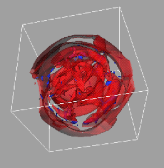
Figure 5.: Magnetic structures. Left: a volume rendering of a snapshot of magnetic field strength (blue/dark isosurfaces) and velocity (red/transparent isosurfaces), from the simulation with $min({\rm Re}_{\rm m})=800$. The magnetic field strength isosurfaces are at a high value relative to the maximum at that instant, and the velocity isosurfaces are at an intermediate value. Right: an average image of the magnetic field obtained by adding three images resulting from the average along the coordinate axis (white corresponds to maximum field strength, and (dark) green to minimum).

No exponential growth can go on forever and eventually the magnetic energy amplification must saturate. To model this non-linear effect, we ran a simulation identical to the kinematic model yielding the result in Figure 3, but including the flow quenching of Eq. (2). Figure 4 shows the evolution of a saturating dynamo, after an initial 25 year exponential growth (identical to that of the purely kinematic simulation): in that case the flow field cycles become less apparent in the evolution of E_m, and a additional long term variations become visible—the dominant period seems to be about 35 years (more than 4.5 cycles). The simulation was terminated after 300 years in Betelgeusian time. One may worry that we have not run the simulation for long enough compared to some dominate diffusion time scale. If diffusion takes place on a time scale related to the largest scale of the system (see e.g. Brandenburg 2001), then the characteristic diffusion time would be $\tau_{\rm d}={\rm R}^{2}/4\pi^{2}\eta\sim 2~{}10^{10}$ years, i.e. longer than the age of the Universe. However, scaling this with our minimum Re${}_{\rm m}=800$ (to its actual value that is on the order of $10^{10}$) yields a diffusion time of $\tau_{\rm d}\sim 1500$ years: that time scale does not presently seem completely inconsistent with our results (see Figure 4), but the simulation covers only a fraction of $\tau_{\rm d}$.

The level of saturation of E_m is effectively set by the choice of the constant kinetic energy density in Eq. (2): thus the model does not contribute any additional knowledge about which field strengths to expect in Betelgeuse.

Figure 6.: Intermittency. Left: the probability distribution function (PDF) for the magnetic field strength (normalized to its maximum) at an instant in the non-saturating kinematic model, corresponding to the snapshot in Fig. 5. Right: power spectrum of the magnetic field strength (full curve). The vertical dashed line indicates the formal resolution limit (the Nyquist wavelength).

But we can, however, study the geometry of the magnetic field that the dynamo generates. Figure 5 (left) shows a volume rendering of isosurfaces of magnetic field structures with a high field strength relative to the maximum: the field becomes concentrated into elongated structures much thinner than the scale of the giant convection cells, but perhaps due to the very dynamic nature of the convective flows, no “intergranular network” is formed (to use solar terminology). The field is highly intermittent (see PDF in Figure 6, left), i.e. only a small fraction of the volume carries the strongest structures. The average magnetic field distribution is illustrated in Figure 5 (right), where it is evident that the field is stratified and decreases in strength from the center of the star to a rather sharp “magnetic surface” at R $\sim 750$ R_⊙. We speculate that the stratification results from the magnetic pumping effect working on the weakest part of the field (cf. Dorch & Nordlund 2001).

The magnetic structures are well resolved, with maximum power on the largest scales above 200 R_⊙ (Figure 6, right). Additionally we observe a slight trend in the topology of the field; fields near (but still below) the surface of the star are predominantly horizontally aligned, while those in deeper layers are radial.

4. Concluding remarks

Based on the results presented here, we may not say conclusively if Betelgeuse does have a magnetic field, of course. The results are tentative and should be used with caution. But we may say that it seems that it can indeed have a presently unobserved magnetic field. The dynamo of Betelgeuse may be characterized as belonging to the class called “local small-scale dynamos” another example of which is the proposed dynamo action in the solar photosphere that may possibly be responsible for the formation of small-scale flux tubes (cf. Cattaneo 1999, but also the discussion by Stein, ibid). However, in the case of Betelgeuse this designation is less meaningful since the generated magnetic field is both global and large-scale.

The future developments of this project will involve firstly using longer time sequences of the input flow field, to avoid having to rely on recycling. Secondly, simulations with higher numerical resolution is currently being carried out (see Freytag & Finnsson, 2002, and Freytag & Mizuno-Wiedner, 2002), which will allow larger runs with higher magnetic Reynolds numbers (i.e. smaller magnetic structures can form). Thirdly, it will be a priority to apply a more realistic quenching expression to introduce the saturation (one that takes into account the relative inclinations of the field and the flow, e.g. the cross-convergence). Lastly, more realistic boundary conditions, and a parameter study with increasing Re_m will be performed. The final goal is to be able to identify the more of operation during the (non-linear) saturation phase of the dynamo at high Re_m in order to predict the likely topology of the magnetic field that one might observe at stars such as Betelgeuse.

Acknowledgments.

SBFD thanks the LOC of IAU Symposium No. 210 for support. The radiation-hydrodynamic simulations yielding the input flow field used in this study was computed at the computing center of the university in Kiel, at the Theoretical Astrophysics Center in Copenhagen, and on the Sun cluster at Ångström laboratory in Uppsala. The dynamo calculations were performed at the Institute for Solar Physics of the Royal Swedish Academy of Sciences.

References

Archontis, V.D., Dorch, S.B.F., & Nordlund, Å. 2002, A&A, accepted

Archontis, V.D., & Dorch, S.B.F. 1999, in Stellar Dynamos: Non-linearity and chaotic flows, ASP conf. series 178, 1

Brandenburg, A. 2001, ApJ, 550, 824

Cattaneo, F. 1999, ApJ, 515, L39

Dorch, S.B.F. 2000, Physica Scripta, 61, 717

Dorch, S.B.F., & Ludwig, H.-G. 2002, Astron. Nachr., 323, in press

Dorch, S.B.F., & Nordlund, Å. 2001, A&A, 365, 562

Freytag, B., & Finnsson, S. 2002, ibid

Freytag, B., & Mizuno-Wiedner, M. 2002, ibid

Freytag, B., Steffen, M., & Dorch, S.B.F. 2002, Astron. Nachr., 323, 213

Galsgaard, K., & Nordlund, Å. 1997, Journ. Geophysical Res., 101, 219

Schrijver, C., & Zwaan, C. 2000, Solar and Stellar Magnetic Activity, CAPS, 34, Cambridge

Stein, R.F. 2002, ibid