Searching for the Signature of the Magnetic Fields at the Base of the Solar Convection Zone with Solar-Cycle Variations of p-Mode Travel Time

Abstract

We study the solar-cycle variations of solar p-mode travel time for different wave packets to probe the magnetic fields at the base of the solar convection zone. We select the wave packets which return to the same spatial point after traveling around the Sun with integral number of bounces. The change in one-bounce travel time at solar maximum relative to minimum is approximately the same for all wave packets studied except a wave packet whose lower turning point is located at the base of the convection zone. This particular wave packet has an additional decrease in travel time at solar maximum relative to other wave packets. The magnitude of the additional decrease in travel time for this particular wave packet increases with solar activity. This additional decrease in travel time might be caused by the magnetic field perturbation and sound speed perturbation at the base of the convection zone. With the assumption that this additional decrease is caused only by the magnetic field perturbation at the base of the convection zone, the field strength is estimated to be about $4-7\times 10^{5}$ gauss at solar maximum if the filling factor is unity. We also discuss the problem of this interpretation.

1 Introduction

Observations give evidence that magnetic fields on the Sun emerge from below. How and where magnetic fields are generated is a long standing unanswered question in astronomy Cowling (1934); Parker (1955); Babcock (1961). It has been suggested that the boundary between the radiative zone and convection zone (CZ) is the best location for an oscillatory solar dynamo Spiegel (1980); Parker (1993); Charbonneau & MacGregor (1997). Many attempts have been made to detect the magnetic fields in this region Gough et al. (1996); Basu (1997); Howe et al. (1999); Basu & Schou (2000); Basu & Antia (2001); Eff-Darwich et al. (2001); Antia et al. (2001). Until now no clear evidence of magnetic field in this region has been found. Here we use the technique of time-distance analysis Duvall et al. (1993) to measure solar cycle variations of travel time of acoustic waves with different ray paths to probe the magnetic fields at the base of the CZ.

A resonant solar p-mode is trapped and multiply reflected in a cavity between the surface and a layer in the solar interior. The acoustic signal emanating from a point at the surface propagates downward to the bottom of the cavity and back to the surface at a different horizontal distance from the original point. Different p-modes have different paths and arrive at the surface with different travel times and different distances from the original point. The modes with the same angular phase velocity have approximately the same ray path and form a wave packet. The relation between the travel time and travel distance of a wave packet can be measured by using the temporal cross-correlation between the time series at two points Duvall et al. (1993).

Different wave packets penetrate into different depths: the wave packet with a larger phase velocity penetrates into a greater depth. Time-distance analysis measures the travel times of different wave packets to probe the interior of the Sun at different depths Duvall et al. (1996); Kosovichev (1996); Kosovichev et al. (2000). The ray path of wave packet computed from a standard solar model with the ray theory for three different phase velocities is shown in Figure 1. If a magnetic field is present at the base of the CZ, it has different effects on different wave packets. It changes the travel time of wave packets which can penetrate into the base of the CZ, while it has no effect on the wave packets which can not reach the base of the CZ. If the magnetic fields at the base of the CZ vary with the solar cycle like the surface magnetic fields, travel time is expected to vary with the solar cycle as well. The change in travel time due to the magnetic fields at the base of the CZ is small because the ratio of magnetic pressure to gas pressure is small. However, the change in travel time increases linearly with the number of bounces between the boundaries of the cavity. Thus the strategy is to measure the change in multiple-bounce travel time. Here we measure the time for a wave packet to travel around the Sun to come back to the same spatial point. If a wave packet takes $N$ bounces to travel around the Sun, the change in travel time would increase by a factor of $N$ relative to the change in one-bounce travel time. Therefore, the problem becomes measuring solar cycle variations of travel time with the auto-correlation function of the time series at the same spatial point. In this study we use two different approaches, the multiple-bounce travel time analysis (MBTTA) and the power spectrum simulation analysis (PSSA), to measure the travel time of wave packets.

2 Multiple-Bounce Travel Time Analysis (MBTTA)

In the first approach (MBTTA), we use the helioseismic data taken with the Michelson Doppler Imager (MDI) on board the SOHO spacecraft Scherrer et al. (1995). The MDI data used here are full-disc low-resolution Doppler images of $192\times 192$ pixels, sampled at a rate of one image per minute. We have analyzed the data in the period of solar minimum and maximum. The data are divided into 4096-minute segments. Each time series of 4096 images is analyzed separately. The procedure of data analysis is described below. (1) Each full-disk Doppler image is transformed into $\sin\theta-\phi$ coordinates, where $\theta$ and $\phi$ are the latitude and the longitude, respectively, in a spherical coordinate system aligned along the solar rotation axis. (2) The differential rotation of the solar surface is removed with an observed surface differential rotation velocity Libbrecht & Morrow (1991). (3) The data are filtered with a Gaussian filter of FWHM = 2 mHz centered at 3 mHz. (4) To reduce the interference among the wave packets of different phase velocities, a phase-velocity filter is applied to isolate the signals in a range of the phase velocity $\omega/[l(l+1)]^{1/2}$, where $\omega$ is the mode angular frequency and $l$ is the spherical harmonic degree. For each time series of 4096 images, the signals in the $(\sin\theta,\phi,t)$ domain are transformed into the $(l,m,\omega)$ domain, where $m$ is the azimuthal order. A filter is applied to select the signals in a range of $\omega/[l(l+1)]^{1/2}$. The center of filter is chosen such that the one-bounce travel distance is $360^{\circ}/N$, where $N$ is an integer. The filtered signals are transformed back to the $(\sin\theta,\phi,t)$ domain. The points inside the active regions are excluded to avoid the contaminated signals measured in the magnetic regions. (5) The auto-correlation function of time series at each $(\sin\theta,\phi)$ is computed. (6) The auto-correlation functions are then averaged over a region of $84^{\circ}\times 94^{\circ}$ at the disk center. The size of averaging area is selected to avoid the signals near the limb. (7) The phase travel time $\tau_{N}$ is determined from the instantaneous phase of the auto-correlation function with a Hilbert transform technique Bracewell (1986); Duvall et al. (1996). It is repeated for $N$ between 6 and 15 to obtain the travel times of different wave packets. Since the waves used to compute the auto-correlation begin at a point at the surface, propagate in all directions to go around the Sun and come back to the same point, the auto-correlation function consists of signals which pass through a medium element from opposite directions. Thus the effects of motion of this element cancel out in the auto-correlation function.

To study solar cycle variations, the travel time $\tau_{N}$ is averaged over a solar minimum period (May 1996 - May 1997) and a solar maximum period (January 2000 - February 2001). It is found that the the travel time at solar maximum is shorter than that at solar minimum. The difference is defined as $\delta\tau_{N}$. The change in one-bounce travel time is equal to $\delta\tau_{N}/N$. To see the change of different wave packets, we plot $\delta\tau_{N}/N$ versus $N$ in the left panel of Figure 2. The result is denoted by the open circles. The value of $\delta\tau_{N}/N$ is approximately the same for all $N$’s, except a small drop at $N=8$. This approximately constant change is caused by the magnetic fields near the surface because the rays paths of different wave packets near the surface are approximately the same. This change in travel time, corresponding to a fraction of change in travel time of about $-1.3\times 10^{-4}$, is consistent with the well-known solar-cycle variations of frequency, about 0.4 $\mu$Hz for modes at 3 mHz Libbrecht & Woodard (1990).

The interesting phenomenon in Figure 2 is the additional decrease in travel time at $N=8$. The average of $\delta\tau_{N}/N$ over all $N$’s except $N=8$ is $-0.763\pm 0.005$ second. The difference between $\delta\tau_{8}/8$ and the average value is $0.053\pm 0.022$ second.

3 Power Spectrum Simulation Analysis (PSSA)

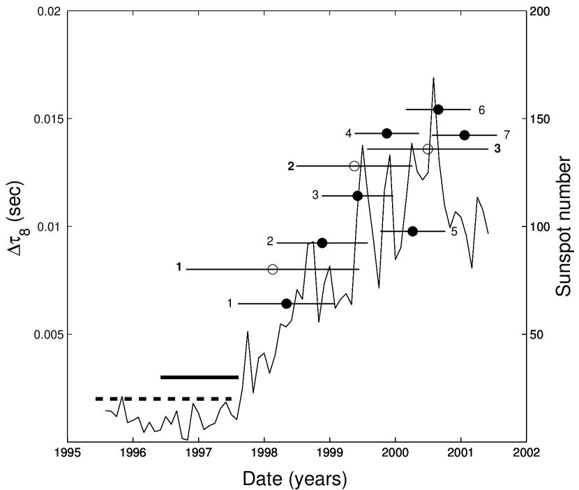
Figure 3: Additional decrease in one-bounce travel time at $N=8$ relative to other $N$’s, $-\Delta\tau_{8}$, from PSSA versus date. The filled circles denote the MDI results, and the open circles the GONG results. The horizontal bar associated with each point indicates the range of period used in averaging the mode frequencies. The number associated with each period is consistent with the number in Figure 2. The thick horizontal line indicates the range of solar minimum period used for MDI, and the dashed line for GONG. The solid line is the sunspot number from the Greenwich Sunspot Data.

The correlation function, from which the travel time is determined, is the inverse Fourier transform of the power spectrum of p-modes. Thus the signal corresponding to the travel time perturbation detected above should also exist in the mode frequencies which are determined from the power spectrum. In the second approach (PSSA), we use the mode frequencies measured with the helioseismic data taken with MDI and the Global Oscillation Network Group (GONG) Harvey et al. (1996) to construct the power spectrum in ($l,\omega$). The MDI data covers May 1996 - June 2001, and the GONG data May 1995 - May 2001. The mode frequencies are averaged over about one year for MDI and about two years for GONG to increase the signal-to-noise ratio. The range of each averaging period is indicated by the horizontal bar in Figure 3. To construct the power spectrum in ($l,\omega$) from the mode frequencies, we assume that the spectral profile of each mode is a Lorentzian, and the width is a function of frequency only. We adopt the width measured in Howe et al. (1999). The power distribution versus $l$ is taken from the $l-\omega$ diagram obtained in MBTTA. The frequency variation of power is obtained by applying a Gaussian filter centered at 3 mHz with FWHM = 0.55 mHz. Power is set zero for frequency greater than 3.5 mHz or smaller 2.5 mHz because some of mode frequencies above 3.5 mHz are not available. The composite power spectrum is filtered with the same phase velocity filter as in MBTTA prior to computing the cross-correlation function with the inverse Fourier transform. The cross-correlation function at zero travel distance corresponds to the auto-correlation function averaged over all spatial points, which is used to determine the travel time of the wave packet. The value of $\delta\tau_{N}/N$ for various periods along the solar cycle is shown in Figure 2.

The results of PSSA also show that there exists an additional decrease in travel time at $N=8$ relative to other $N$’s. The magnitude of additional decrease increases with solar activity. To quantify the additional decrease at $N=8$, we define $\Delta\tau_{8}$ as the difference between $\delta\tau_{8}/8$ and the value at $N=8$ determined from a linear fit to $\delta\tau_{N}/N$ of all other $N$’s. Figure 3 shows $-\Delta\tau_{8}$ and the sunspot number versus date. The results of MDI and GONG are consistent, though the results of GONG are noisier. At solar maximum, $-\Delta\tau_{8}\approx 0.015$ second which is smaller than that from MBTTA. This difference may be caused by the differences in data analysis. First, the width of the frequency filter used in PSSA is smaller than that in MBTTA because some of higher mode frequencies are not available. A narrower filter yields a wider wave packet. Second, the correlation functions are averaged over a central region of $84^{\circ}\times 94^{\circ}$ in MBTTA, while the averaging area in PSSA is equivalent to the area used to measure the mode frequencies, which is almost the entire disk. The signals near the limb have a lower signal-to-noise ratio. Third, the active regions are excluded in MBTTA, while they are not in PSSA.

4 Discussion

To test whether the shorter travel time at $N=8$ is caused by the analysis procedure, we did the following test. The frequency difference between solar maximum and minimum is smoothed by a fit in the ($l,\nu$) domain. The mode frequencies at solar maximum are simulated by adding this smooth function to the mode frequencies at minimum. Applying the same procedure as in PSSA to the measured frequencies at solar minimum and the simulated frequencies at solar maximum, we compute the change in travel time for different $N$’s. The result shows that the change in travel time is approximately the same for all $N$’s and there is no additional decrease at $N=8$. This test indicates that the shorter travel time at $N=8$ is not caused by the analysis procedure.

It is unlikely that the shorter travel time at $N=8$ is caused by the spatial distribution of the near-surface magnetic fields. The most prominent spatial pattern of magnetic activity on the surface is the active latitudinal band in each hemisphere. The separation between the centroids of two active bands is about $42^{\circ}$ in 1998 and monotonically decreases to about $29^{\circ}$ in 2000 (from Greenwich Sunspot Data). If the latitudinal distribution of active regions can cause an additional decrease in one-bounce travel time, it would occur at $N=9$ in 1998 and shift to $N=12$ in 2000. This contradicts to the PSSA results shown in Figure 2. Thus it is unlikely that the shorter travel time at $N=8$ is caused by the separation of two active latitudinal bands on the surface. Since the active longitudes is less prominent than the active latitudes, it is unlikely the anomaly at $N=8$ is caused by the active longitudes.

The fact that the ray path of the wave packet of $N=8$ has the lower turning point at the base of the CZ as shown in Figure 1 suggests that the additional decrease in travel time at $N=8$ may be caused by the solar-cycle varying wave speed at the base of the CZ. The change in wave speed at the base of the CZ could be caused by magnetic field perturbation or/and sound speed ($[\gamma p/\rho]^{1/2}$) perturbation. It has been shown that the global measurements can not distinguish these two effects Zweibel & Gough (1995). The previous study Kosovichev & Duvall (1997) has also indicated that either magnetic field perturbation or sound speed perturbation alone would cause a change in travel time not only for $N=8$ but also for $N<8$, though it is smaller. Thus either magnetic field perturbation or sound speed perturbation alone can not explain the measurements of travel time variation shown in Figure 2. However, the combination of these two perturbations might be able to explain the measured travel time variations. Although we do not know the mechanism producing the sound speed perturbation, it probably has the magnetic origin because the presence of a magnetic field could change the thermal structure and leads to a change in sound speed.

With the above caution in mind, we will estimate the field strength based on the assumption that the additional decrease in travel time at $N=8$ is caused only by the magnetic fields at the base of the CZ. If we adopt the value of $\Delta\tau_{8}$ measured with MBTTA and PSSA, the fraction of change in travel time due to the wave speed perturbation at the base of the CZ is about $0.015/\tau_{8}-0.053/\tau_{8}\approx 2.6-9\times 10^{-6}$. If we use the half width of the tachocline, $0.025R_{\odot}$, as the width of the magnetic layer at the base of the CZ Corbard et al. (2001), the fraction of change in wave speed at the base of the CZ, $\delta w/w$, is about $2.6-9\times 10^{-5}$ because the wave packet of $N=8$ spends about one tenth of time inside the tachocline. If the change in wave speed is entirely due to the presence of magnetic fields, the fraction of change in wave speed is $\delta w/w=\sin^{2}\theta(v^{2}_{A}/c^{2})/2$, where $v_{A}=B/(4\pi\rho)^{1/2}$ is the Alfven speed, and $\theta$ is the angle between wave propagation direction and magnetic field Kosovichev et al. (2000). The density $\rho\approx 0.2$ g cm^-3 in the tachocline. Averaging $\sin^{2}\theta$ over all directions yields about 1/2. Thus the magnetic field strength $B\sim[16\pi\rho c^{2}(\delta w/w)]^{1/2}\sim 4-7\times 10^{5}$ gauss if the filling factor of magnetic field is unity. A smaller filling factor would increase the estimated field strength. The field strength estimated here is greater than most theories predict Fisher et al. (2000). Such a strong field needs a large degree of subadiabaticity in the tachocline to stabilize it Gilman (2000). The approximately constant $\delta\tau_{N}/N$ at $N\geq 9$ suggests that there is no strong magnetic field in the middle of the CZ.

The problem of above interpretation is that no additional decrease in travel time is detected for the neighboring wave packets of $N=8$ in our measurements. The neighboring wave packets, $N=7$ and 9, may be also influenced by the magnetic fields at the base of the CZ. The influence depends on the width and location of the magnetic layer at the base of the CZ and the width of the wave packets. If we adopt the parameters used above and the ray approximation to estimate the influence on the neighboring wave packets, the additional decrease at $N=7$ is about $40\%$ of that at $N=8$, while there is no effect on $N=9$. However, the finite width of the wave packets would increase the effect of magnetic fields on the neighboring wave packets. The previous studies have shown that the travel-time sensitivity kernel is wide Jensen et al. (2000); Birch & Kosovichev (2000). To estimate the effect due to the finite width, we construct the 3-D wave packet by superposing the eigenfunctions of the modes consistent with our phase-velocity filter Bogdan (1997). The FWHM of the energy distribution in the radial direction for the wave packets of $N=7$ and 9 at the lower turning point is about $0.1R_{\odot}$, which is greater than the separation between the lower turning points of two neighboring wave packets, about $0.02-0.03R_{\odot}$. Thus the influence of magnetic fields at the base of the CZ on the wave packets of $N=7$ and 9 is not negligibly small compared with that on $N=8$. This contradicts to the result of our measurements. At this moment, we do not know how the combination of magnetic field perturbation and sound speed perturbation can help resolve this contradiction.

Figure 1: Diagram showing ray paths of three different wave packets computed from a standard solar model Christensen-Dalsgaard et al. (1996) with the ray approximation D’Silva & Duvall (1995). The thick solid line is the solar surface, and the dashed line is the base of the CZ at $0.713R_{\odot}$ Basu (1997). Ray 1, which takes 15 bounces to go around the Sun, is not affected by the magnetic fields at the base of the CZ. Ray 2, taking 8 bounces to go around the Sun, has the lower turning point very close to the base of the convection zone. Ray 3, taking 5 bounces to go around the Sun, can penetrate into the radiative zone.

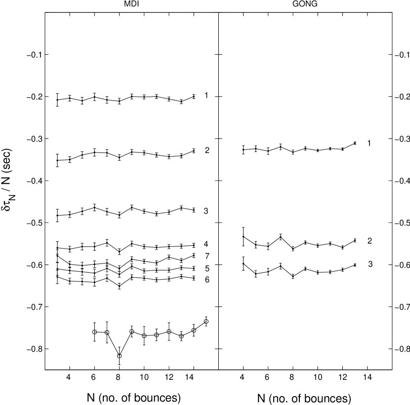
Figure 2: Change in one-bounce travel time relative to solar minimum versus number of bounces $N$, which corresponds to different wave packets. The result from the multiple-bounce travel time analysis (MBTTA) is denoted by the open circle in the left panel. The error bar is an estimate of fluctuation from averaging the travel time of different time series over solar minimum or maximum, corrected for variations of solar activity. The result from the power spectrum simulation analysis (PSSA) is denoted by the filled circle. The left panel is computed from the MDI mode frequencies, and the right panel from the GONG mode frequencies. The sequence of the averaging periods is indicated by the number associated with each curve. The range of each period is indicated by the horizontal bar of each point in Figure 3. The error bar of PSSA is estimated from Monte Carlo simulations using the errors in mode frequencies.

References

- Antia et al. (2001) Antia, H. M. et al. 2001, MNRAS, 327, 1029
- Babcock (1961) Babcock, H. W. 1961, ApJ, 133, 572
- Basu (1997) Basu, S. 1997, MNRAS, 288, 572
- Basu & Schou (2000) Basu, S. & Schou, J. 2000, Sol. Phys., 192, 481
- Basu & Antia (2001) Basu, S. & Antia, H. M. 2001, in Proc. SOHO 10/GONG 2000 Workshop: Helio- and Astero-seismology at the Dawn of the Millennium, ed. A. Wilson (ESA SP-464; Noordwijk: ESA), 297
- Birch & Kosovichev (2000) Birch, A. C. & Kosovichev, A. G. 2000, Sol. Phys., 192, 193
- Bogdan (1997) Bogdan, T. J. 1997, ApJ, 477, 475
- Bracewell (1986) Bracewell, R. N. 1986, The Fourier Transform and Its Applications, 2nd ed. (New York: Mc-Graw-Hill), 267-272.
- Charbonneau & MacGregor (1997) Charbonneau, P & MacGregor, K. B. 1997, ApJ, 486, 502
- Christensen-Dalsgaard et al. (1996) Christensen-Dalsgaard, J. et al. 1996, Science, 272, 1286
- Corbard et al. (2001) Corbard, T., Jimenze-Reyes, S. J., Tomczyk, S., Dikpati, M., & Gilman, P. 2001, in Proc. SOHO 10/GONG 2000 Workshop: Helio- and Astero-seismology at the Dawn of the Millennium, ed. A. Wilson (ESA SP-464; Noordwijk: ESA), 265
- Cowling (1934) Cowling, T. G. 1934, MNRAS, 94, 39
- D’Silva & Duvall (1995) D’Silva, S. & Duvall, T. L. Jr. 1995, ApJ, 438, 454
- Duvall et al. (1993) Duvall, T. L. Jr., Jefferies, S. M., Harvey, J. W., & Pomerantz, M. A. 1993, Nature, 362, 430
- Duvall et al. (1996) Duvall, T. L. Jr., D’Silva, S., Jefferies, S. M., Harvey, J. W., & Schou, J. 1996, Nature, 379, 235
- Eff-Darwich et al. (2001) Eff-Darwich, A., Perez Hernandez, F., & Korzennik, S. G. 2001, in Proc. SOHO 10/GONG 2000 Workshop: Helio- and Astero-seismology at the Dawn of the Millennium, ed. A. Wilson (ESA SP-464; Noordwijk: ESA), 289
- Fisher et al. (2000) Fisher, G. H., Fan, Y., Longcope, D. W., Linton, M. G., & Pevtsov, A. A. 2000, Sol. Phys., 192, 119
- Gilman (2000) Gilman, P. A. 2000, Sol. Phys., 192, 27
- Gough et al. (1996) Gough, D. O. et al. 1996, Science, 272, 1296
- Harvey et al. (1996) Harvey, J. W. et al. 1996, Science, 272, 1284
- Howe et al. (1999) Howe, R., Komm, R., & Hill, F. 1999, ApJ, 524, 1084
- Jensen et al. (2000) Jensen, J. M., Jacobsen, B. H., & Christensen-Dalsgaard, J. 2000, Sol. Phys., 192, 231
- Kosovichev (1996) Kosovichev, A. G. 1996, ApJ, 461, L55
- Kosovichev & Duvall (1997) Kosovichev, A. G. & Duvall, T. L. Jr. 1997, in Solar Convection and Oscillations and Their Relationship, ed. P. F. Pijpers & J. Christensen-Dalsgaard (Dordrecht: Kluwer), 241
- Kosovichev et al. (2000) Kosovichev, A. G., Duvall, T. L. Jr., & Scherrer, P. H. 2000, Sol. Phys., 192, 159
- Libbrecht & Woodard (1990) Libbrecht, K. G. & Woodard, M. F. 1990, Nature, 345, 779
- Libbrecht & Morrow (1991) Libbrecht, K. G. & Morrow, C. A. 1991, in Solar Interior and Atmosphere, ed. A. N. Cox et al. (Tucson: Univ. Arizona Press), 479
- Parker (1955) Parker, E. N. 1955, ApJ, 122, 293
- Parker (1993) Parker, E. N. 1993, ApJ, 408, 707
- Scherrer et al. (1995) Scherrer, P. H. et al. 1995, Sol. Phys., 160, 237
- Spiegel (1980) Spiegel, E. A. & Weiss, N. O. 1980, Nature, 287, 616
- Zweibel & Gough (1995) Zweibel, E. G. & Gough, D. O. 1985, in Proc. Fourth SOHO Workshop: Helioseismology, ed. J. T. Hoeksema (ESA SP-376; Noordwijk: ESA), Vol. 2, 73